Dynamic Behavior and Deposit Features of Debris Avalanche in Model Tests Using High Speed Photogrammetry

Abstract

Model tests of debris avalanche can not only illuminate formation mechanisms but also represent deformation and motion processes. At present, the static terrain data of model tests are measured before and after experiments using terrestrial laser scanning. To study the motion and deformation of research objects, it is necessary to explore new techniques to obtain dynamic terrain data in the course of experimentation. In this paper, taking specified experimental tests of debris avalanche as an example, the method of 4D reconstruction using high-speed close-range photogrammetry is described in detail. The dynamic terrain data of model tests were obtained after the data were processed. Then, the dynamic behavior and deposit features of debris avalanche were analyzed in detail. Results show that dynamic terrain data of model tests can be obtained rapidly and accurately with this method. The propagation and deposit processes of the debris avalanche have evident stage characteristics, which can be divided into the starting, acceleration, constant, and deceleration stages. The granular size, slope angle, and barrier effect have a great influence on the travel distance and duration of the debris avalanche. The depth of the intermediate and leading area of the debris avalanche increased gradually and the depth of the trailing area first increased then decreased. We believe that this approach can also be applied to other domains involving the acquisition of dynamic terrain data and, thus, deserves to be applied widely.

1. Introduction

Landslides, earthquakes, floods, and other natural hazards occur frequently in mountain areas, where they damage construction, transportation systems, the infrastructure of city, town and population centers, and threatens the life of many people [1,2]. The study of the dynamic behavior and deposit features of these hazards is very significant in reducing the loss of life and property; this will contribute to sustainable development of economy and society in mountain areas. At present, the monitoring of natural hazards mainly uses a variety of monitoring devices such as Interferometric Synthetic Aperture Radar (InSAR), unmanned aerial vehicles (UAVs), rain gauges, displacement sensors, Global Navigation Satellite System (GNSS), water pressure sensors, water level meters, etc. [3,4]. Their task is to collect the data before the movement of natural hazards begins; however, data on movement stages can be hard to obtain. The method of numerical simulation is a relatively accurate and practical method of acquiring dynamic terrain data in model tests [5], but it is still not widely accepted in geotechnical engineering and engineering geology as some important parameters are not necessarily considered accurate.

Model tests are likewise an important method of quantitative research on the formation mechanism of natural hazards whose results also can reflect the dynamic behavior and deposit features induced by natural hazards, which are widely accepted and used in the field of geological hazards, including base friction test apparatus [6], rotating drum experiments [7,8], centrifuge model tests [9,10,11,12], normal gravity experiments [13,14], etc.; however, acquiring data accurately is a key problem of the system. Some process variables, such as pressure, temperature, water level variables, etc., may be obtained by data collection devices. Static terrain data can be measured before and after experiments by terrestrial laser scanning [15,16]. The projected fringe method and stereo photographic systems (such as 3D Camera Sensor and 3D Optical Measurement Services) are two main methods that may be employed to acquire dynamic terrain data. The projected fringe method documents transient states as contour lines generated by projecting horizontal lines on the inclined plane and relates the deformation of the lines to surface elevation. The projected fringe technique can be used for the mapping of surface topography and measurement of surface deformations [17]. For example, it can be used for measuring the evolution of avalanches from their initiation to their deposit [18]. The accuracy in the value of the resolution depends on the spacing of the projected fringe; it is generally poor. 3D camera sensor (e.g., Microsoft Kinect, Asus Xtion, Primesense Carmine, etc.) may also be used to document dynamic terrain data that researchers can apply to study the impact of granular movement subjected to different obstacles [19]. Unfortunately, data resolution at 640 × 480 at 30 frames per second (FPS) is limited by the size of the sensor and its accuracy is still insufficient. This applies to partial regions with relatively slow speed. If the method is used to acquire the data of an entire target region, the value of the resolution is further significantly reduced. Meanwhile, 3D optical measurement services can also capture dynamic processes three-dimensionally and analyze them regarding geometric changes. For example, MoveInspect HF can collect data without time limits at a frequency of up to 1000 Hz. However, these data acquisition systems are very expensive and mainly used in industrial photogrammetry (such as vehicle dynamics testing), according to Luhmann [20]. Therefore, it is necessary to explore new techniques to obtain dynamic terrain data in the course of the model testing.

Photogrammetry is the most common method, traditionally, it is only used to obtain the static data of a target zone with a single camera. For example, it has been widely used in the fields of archaeology [21,22], cultural heritage conservation [23], architecture [24], hydraulic engineering [25], physical geography [26], engineering geology [27], etc. The need for multiple synchronized high-speed cameras and limitations of a large data-processing capacity deter the implementation of photogrammetry at a high temporal rate. As digital cameras with increasingly higher frame-rates become available, the dynamic range of the velocity measurements can be expanded and higher velocities can be measured for target zones in time-varying scenes [28]. These methods have been applied to monitor the dynamic stresses and strains of wind turbines [29,30,31], obtain the structural dynamic properties of civil structures [32,33], and measure the vibrations of mechanical equipment among other applications [34]; however, there are few applications in geotechnical engineering and engineering geology.

James and Robson [35] calculated the volume changes of lava flows through generated point clouds from images captured once a minute for 37 min. Eltner et al. [36] performed two field tests to study soil surface changes at 15-s intervals because of their relatively slow speed, which can facilitate data acquisition in a normal manner. Several existing studies on the soil erosion and debris flow of flume tests have been devoted to obtaining the dynamic terrain data of model tests; however, their temporal resolution usually reaches levels only from several seconds to a few minutes [37,38,39]. The potential of topographic data with high temporal resolution is still far from being fully utilized. With the development of image processing technology and ability of digital cameras, high-speed close-range photogrammetry could be applied to acquire dynamic terrain information in model tests.

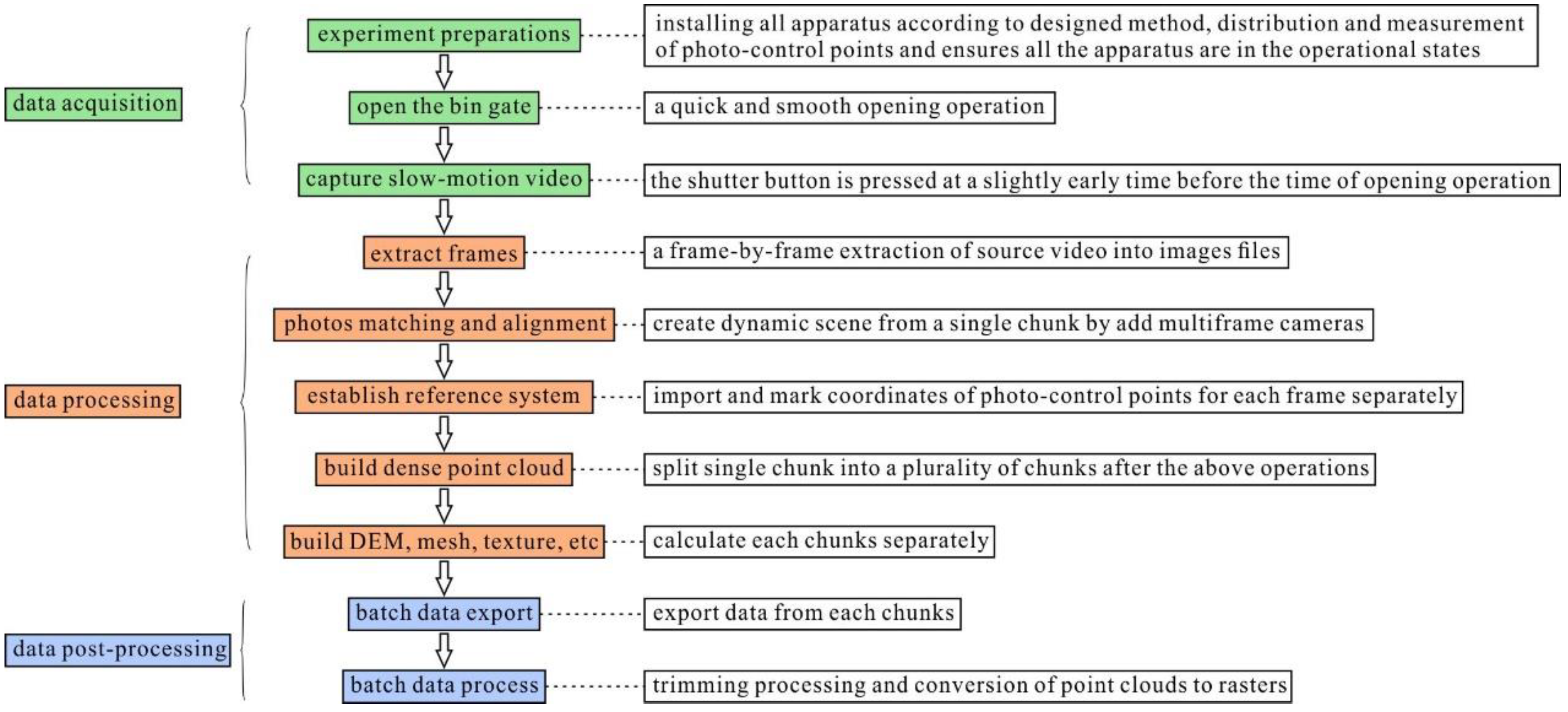
In this study, an approach is presented for the 3D (or 4D) reconstruction of dynamic scenes in model tests. The setup of the image acquisition scheme is displayed in detail and the raw experimental data are treated to obtain the required physical variables. Based on these physical variables, several important conclusions can be drawn.

2. Experimental Cases

2.1. Chute Construction

The constructed chute is comprised of four sections connected via six hinges that may be set to any desired angle through six U-shaped clips on the top of the apparatus. The storage bin is positioned on the upper portion of the chute. The bin gate is opened and closed through the pull and plug method. Moreover, the outlet end of the chute remains open, allowing the debris to exit freely along its longitudinal axis. Each separate chute has a width, depth, and height of 500, 223, and 250 mm, respectively. The internal dimensions of the storage bin are 300 × 223 × 250 mm. The chute is formed of 8-mm thick acrylic plates. The front wall incorporates a membrane to avoid any interfering reflections on the digital cameras. The back wall has graph paper with 10 × 10 mm squares, which facilitates the post-image identification. The bottom surface has a variety of different patterns printed, which improve the quality of the obtained measuring results. The perspective view of the chute is shown in Figure 1.

2.2. Experimental Facility and Layout

Three Sony DSC-RX100M5 digital cameras are mounted on top of the chute apparatus to record super slow-motion videos during the experiment. The time is measured by a millisecond stopwatch timer throughout the experimental process. The dynamic behavior and deposit features of the experiment are recorded by a Nikon D750 DSLR camera, which is mounted on a tripod on the right side of the chute. To verify the availability and applicability of the method, a number of parallel and equally spaced fringes are projected onto the bottom surface of the chute via a laser projector. A certain number of photo-control points must be distributed in the camera’s fields of view so that the experimental data can be oriented in a defined coordinate system. The visual perspective of the experimental facility is shown in Figure 2.

2.3. Grouping

To analyze the influence of granular size, slope angle, and barrier effect, the experiment is divided into eight groups to analyze the dynamic behavior and deposit features under different experimental conditions (

Table 1. Group of experiments where the main factors considered are the granular diameter, slope shape, and position of barrier.

Experiments Nos.	Granular Diameter	Slope Shape	The Position of Barrier
Experiment 1	Fine gravel	A	No
Experiment 2	Quartz sand	A	No
Experiment 3	Fine gravel	B	No
Experiment 4	Quartz sand	B	No
Experiment 5	Fine gravel	B-1	Upper area
Experiment 6	Fine gravel	B-2	Lower area
Experiment 7	Fine gravel	C	No
Experiment 8	Quartz sand	C	No

).

Two different granular diameters are chosen as the experimental object. These are the granular diameters of polished gravel ranging from 4 to 6 mm (Figure 3a) and of quartz sand of approximately 30 mesh (Figure 3b). At a debris weight of 22.4 kg, the volume of fine gravel is 13,997.1 cm³ and the volume of quartz sand is 17,535.6 cm³.

The slope angle is fixed at several values to study the dynamic and deposit behaviors of debris. Different shapes are employed, respectively, from A to C. Shape A has evident buffering units at the second and third slopes; the slope angles are 36.3°, 19.7°, 8.7°, and 17.9° from top to bottom. The slope angles of shape B are 34.4°, 26.6°, 14.5°, and 7.9° from top to bottom, making the transition relatively smooth. Shape C is held at a constant 19.9° angle at all times. Spherical crown-shaped barriers are provided at upper and lower portions on the bottom surface of the chute. The radius and height of the spherical crown are 45 mm and 35 mm, respectively. The coordinates of the center of the upper and lower spherical crown are (x, y) = (800, 540) mm and (x, y) = (1300, 365) mm, respectively. The regions where the barriers are located present slopes of approximately 26.6° and 14.5°, respectively. The slope profiles of the chute are shown in Figure 4.

3. Methods

Data acquisition, processing, and post-processing are discussed below. The entire workflow of data acquisition and processing is illustrated in a flowchart (Figure 5), and the actual work images are shown in Figure 6.

3.1. Data Acquisition

The experimental materials and apparatus were prepared according to a previously designed method. All the apparatus (millisecond stopwatch timer, the laser projector, D750 camera, etc.) were confirmed to be in operational states. Moreover, it is necessary to distribute and measure photo-control points in advance. Any measuring instrument can be used to measure the coordinates of the photo-control points to reach the desired accuracy. In this study, these values were measured with a total station resulting in millimeter accuracy. In addition, the three DSC-RX100M5 digital cameras above the chute apparatus were set to the same parameters before the start of the experiment. The super slow-motion videos during the experiment were recorded with the digital cameras in the high frame rate (HFR) mode. Slow motion video in each group were obtained from three DSC-RX100M5 digital cameras (Figure 6a). The camera specifics of this experiment are listed in

Table 2. Camera specifications throughout the data collection course.

Items	Parameters
Sensor type	1.0-type (13.2 mm × 8.8 mm)
Shooting mode	HFR mode (shutter speed priority)
Recorded Pixels	1920 × 1080@250 fps
Effective Pixels	1824 × 1026@250 fps
Recordable duration	approx. 4 s (quality priority)
Focal length	26 mm (35 mm equivalent)

. Experimental duration is from approximately 1.5 to 2 s but only 3–7 s of recordable duration was retrieved from the cameras in HFR mode. The video must record all experimental phenomena, completely. Thus, the shutter button needs to be pressed at a slightly early time before the opening operation.

3.2. Data Processing

Before the 4D reconstruction, the frame-by-frame extraction of the source video into images files must be completed (Figure 6b). There are numerous software programs implementing these functions currently on the market. So far, a major reason for the limited implementation of photogrammetry at a high temporal rate is the lack of a multi-sensor synchronization image capture systems. To solve this problem, the millisecond stopwatch timer is first used to measure the synchronization data in this study, that is, a set of images extracted from the source video at the same point in time may be grouped to belong to one group. Each set of images can create a 3D scene at that point in time by the photogrammetric software.

Currently, the main photogrammetric software on the market are Smart3D Capture, Pix4Dmapper, and Agisoft Metashape among others. Agisoft Metashape can be used for 4D reconstruction by adding multiframe cameras and allows for the creation of batch procedural control due to an Integrated Development Environment (IDE) using the Python programming language, making it an optimal option. First, it is necessary to create a single chunk by adding multiframe cameras, making the coordinate marking of photo-control points for each frame much easier. In the next step, one should import and mark the coordinates of the photo-control points for each frame separately. If there are significant changes in the location of the digital cameras, we suggest splitting the single chunk into a plurality of independent chunks after these operations. Subsequently, a series of spatial data (point cloud data, digital elevation model (DEM), mesh, texture, etc.) could be reconstructed for each frame by each chunk separately (Figure 6c).

In this experiment, frame rates are recorded during the experiments. The temporal resolution is 4 milliseconds and the data collection at this rate yields up to 500 sets of data within two seconds. Such a significant volume of data poses a great challenge to subsequent processing. Likewise, it is not necessary to observe what happens at every time point. The value of the predetermined time interval is set to 40 milliseconds; that is, data processing can be performed every 10 frames.

3.3. Data Post-Processing

After this processing is complete, the spatial data of each chunk can be exported separately. These data include information on debris surface, chute, additional apparatus, etc.; however, we are only interested in the debris’ surface changes. Here, trimming processing is performed prior to outputting the data. Direct processing in the software is a slow and tedious process and scripts can be used to perform this task automatically in PolyWorks. The 3D spatial sequence data after trimming processing is shown in Figure 6d. Next, the conversion of point clouds to rasters is performed in ArcGIS, which also allows for the creation of batch procedural control that can be realized using the Python programming language. These methods are fast, efficient, and convenient.

4. Results

Although the results indicate suitable reproducibility, there is always some deviation for various reasons. To avoid this problem, each experiment is repeated over three times and the optimal one is selected to be used for 4D reconstruction. There are no significant differences in the travel distance and duration of experiment.

4.1. 3D Spatial Data

3D spatial data at a certain point in time include point cloud data, DEM, mesh, texture, etc. as seen in the results of Experiment 6 at 840 ms shown in Figure 7. In this example, the pixel resolution reaches 1.19 mm/pix and the precision of this method is comparably high, sufficient to capture the textural details of the debris surface. The above spatial data may be chosen according to the application requirements. Here, the point cloud data are chosen to systemically study the dynamic behavior and deposit features of the debris avalanche.

4.2. Accuracy Assessment

To verify the accuracy of the method, points R₁ to R₃ are affixed to the chute and selected as reference points for the accuracy assessment. For example, in Experiment 4, the coordinate values were measured with a total station. Their coordinates were R₁(1.2934, 0.5592, 0.6210), R₂(1.1167, 0.8461, 0.6703), and R₃(1.5647, 0.8493, 0.5497), respectively. The residual error from the spatial data at the same position is shown in Figure 8. The residual level of R₃ is lower than those of R₁ and R₂. This is because the distances from the fixed point of the chute are different; R₃ is located close to the fixed point of the chute leading to the vibration width of position R₃ being smaller than the other two. The impingement stream in the x-direction is due to debris movement along the x-axis. Thus, the residual level in the x-direction is greater than in the y- and z-directions for R₁ and R₂.

The root mean square (RMS) values of the residual error were also calculated as RMS₁(0.0047, 0.0010, 0.0012) m, RMS₂(0.0036, 0.0005, 0.0020) m, RMS₃(0.0015, 0.0005, 0.0022) m, respectively. The data precision is in the millimeter range, meaning that the accuracy of the method is at the same level as the total station resulting in millimeter accuracy and that it can be employed in the model test.

4.3. Method Comparison

To verify the availability and applicability of the method, the terrain data from the projected fringe method were compared with the photogrammetry results. The application of the projected fringe method has been widely used in the fields of manufacturing, medical sciences, computer sciences, homeland security, and entertainment [40,41]. The basic operating principle of this method is to capture transient states as contour lines generated by projecting horizontal lines on an inclined plane via a laser projector, relating the deformation of the lines to surface elevation. The data acquisition workflow is illustrated in Figure 9.

As shown in Figure 10, three different types of data are presented at several points in time. The photogrammetric data have more texture information. Although this method may acquire more precise topographical data by increasing the number of fringes, further improvements in its accuracy cannot be expected because of the width of these fringes. In this experiment, the width and space of these fringes are approximately 5 and 20 mm, respectively. The fringe projection DEM data have a clear stair-step shape. In particular, the terrain data cannot be reflected in the shape features of the barrier areas as it is completely distorted.

5. Discussion

Dynamic terrain data can be documented in model tests by the method described above. The analysis of these data can draw forth many new conclusions beneficial for experimental studies. In addition, several things should be noted before initiating analysis: first, the experiment end time criterion based on the running of trailing debris is its stoppage rather than the leading portion. This is because the deposit range is quite diverse and highly random in the leading area, especially in the polished gravel experimental group. Moreover, sometimes when the leading debris continues to move, the trailing debris has already come to a full stop. Specifically, the particle image velocity (PIV) technology developed in MATLAB is used to estimate the differences in the two adjacent images [42], the end time of the experiment is identified when the amount of deformation reaches zero (approximately zero). Second, the following granular volume only includes the debris outside the bin gate. Finally, the depth of the debris is the vertical distance (z-direction) from that point to the bed of chute, not the shortest distance along the normal direction. Similarly, the volume of the debris is the deposition volume at specific time points.

5.1. Temporal Evolution of Volume

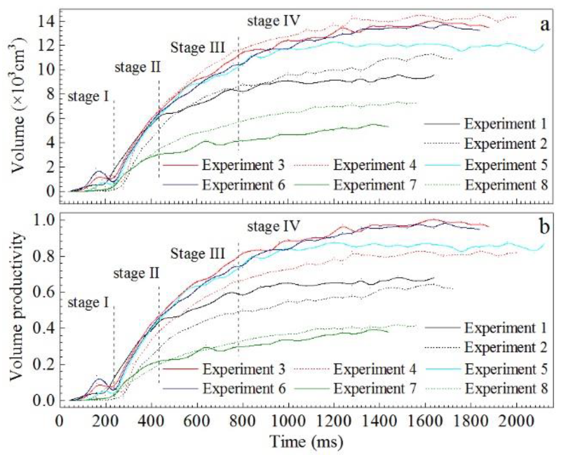
After performing a series of subtraction operations between the transient states and initial slope in ArcGIS using Python to create a batch of procedural controls, the temporal evolution of volume can be easily obtained. As shown in Figure 11, with the debris continuously passing from the bin gate, the volume also increases. The propagation and deposit processes have evident stage characteristics, which can be divided into the starting, acceleration, constant, and deceleration stages. At the starting stage (stage I), the time consumption of the bin gate from start to end is approximately 120 ms and the volume of the debris increases relatively slowly as the opening area is gradually increased. In the second stage (stage II), after the bin gate is fully opened, the volume of debris growth accelerates. When the curve reaches a steady-state, the volumetric growth rate of the debris has remained relatively stable (Stage III). At the deceleration stage (stage IV), as the travel distance continues to increase and the debris loses energy, the volume changes appear at a slower rate.

It should be noted that an anomaly appeared at the time range of approximately 120–240 ms. Particularly, this phenomenon is marked for Experiment 3 and Experiment 6. These video materials indicate a specific phenomenon in these experiments where the bin gate obstructs the view of the digital cameras for approximately 120 s after the gate is pulled up to a certain height. During this time, the debris imaging data are not complete.

It was found that the granular size, slope angle, and barrier effect have a great influence on the dynamic behavior and deposit features of the debris. As shown in Figure 11a, the effect of slope angle is particularly marked. The volume and duration of the debris for slope B (Experiment 4–6) reached maximum values in three kinds of slope shape, their sequence is slope B > slope A > slope C. The shape of the slope B is like a curve bending downwards. The variety of debris movement is sufficiently accelerated as the two upper sections of the chute have a relatively large tilt angle. Furthermore, the smooth transitional section at the bottom of the slope could help debris deposit in a step-by-step manner. Slope A underwent a similarly accelerated movement but there was an unloading platform with an inclination of 8.7 degrees when the debris reached the third section, a mass of debris obstructed the back of the plate as the energy loss increased. Each section of slope C had the same tilt angle. As the debris did not undergo any acceleration stage, it had a limited volume and duration. Additionally, the influence of granular size cannot be ignored. Generally, the groups of coarse grains (fine gravel) had similar short movement time and small volume characteristics, while the groups of fine grains (quartz sand) showed the opposite. As shown in Figure 11b, for slopes A and B, the volume productivity (the ratio of the outlet gate volume to the initial volume) had significantly different characteristics. The volume productivity of coarse grains had larger than fine grains. For the slope C, although the ultimate productivity of the coarse grains was low compared to the fine grains, the productivity of the two groups only differed slightly. The productivity of coarse grains was better than that of the fine grains. This is probably because the energy of the coarse grains was easily transferred and the energy dissipation was smaller than in fine grains. The single polished gravel had a greater mass and volume, which rolled easily, causing the deposit range to be quite diverse and the travel distance to be random.

Additionally, the position of the barrier is also another factor impacting the volume and duration of the debris, as displayed in Figure 11a,b. The barrier of Experiment 5 was fixed in a high position and the volume of the debris was smaller than in Experiment 3 (no barrier) due to the debris meeting the barrier at the initial stage. The duration of the debris was much longer in the presence of a barrier. The barrier of Experiment 6 was fixed in a low position (near the leading area) and there was little adverse influence on the propagation and deposit of the debris. It was further envisaged that the barrier factors such as position, shape, size, etc., have a significant effect on the dynamic behavior and deposit features. The detailed analysis of these influencing factors can help provide better advice for the design and evaluation of dams.

5.2. Time-Course Analysis of Sampling Probe

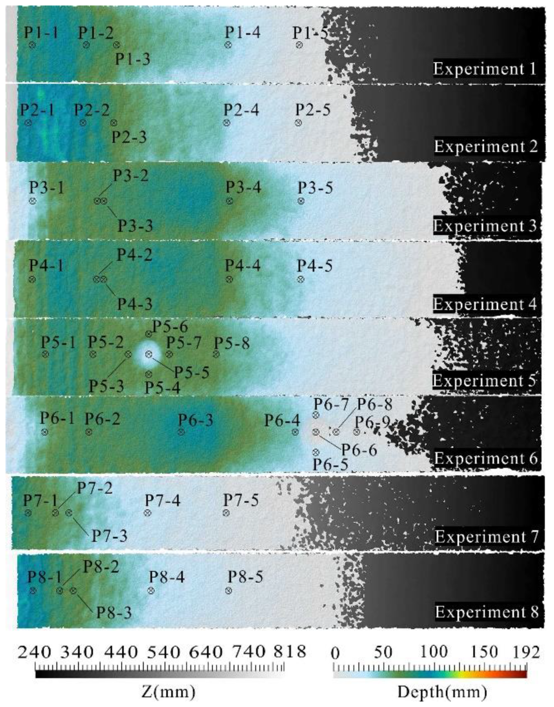
Another important task was to extract the time-course data from certain points. The location of these certain points is schematically shown in Figure 12; these include representative sampling points, binding points, the top of the spherical crown, and areas nearby.

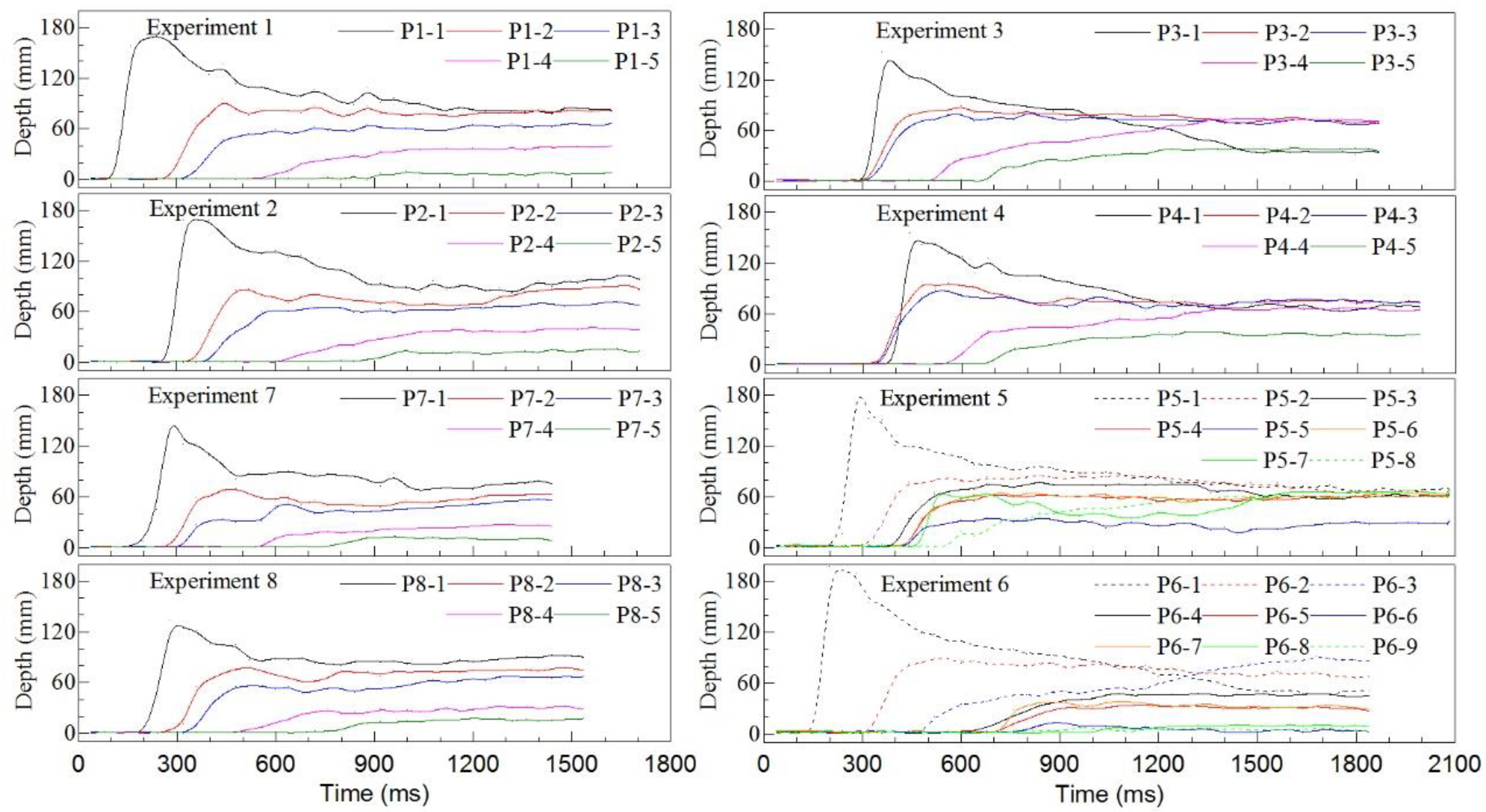
The time-course curves of the sampling probe are shown in Figure 13. The relatively large differences between these curves were discovered by analyzing data from all the experimental groups. For Experiments 3 and 6 (the volume productivity close to 1.0), the depth of the rear sampling probe (P3-1 and P6-1) was subjected to a rapid increase followed by a gradual decline; the binding point (P3-2 and P6-2) remained constant after reaching its maximum; the change of the middle sampling probe (P3-4 and P6-3) consisted of a fast increase followed by a slow increase; and the value of the front sampling probe (P3-5 and P6-4) was the same as the binding point growth rate. For the other experimental groups (volume productivity less than 1.0), the time-course curves of some sampling probe were quite different from Experiments 3 and 6. For example, in Experiment 1 (fine gravel), the depth of the rear sampling probe (P1-1) rapidly increased and appeared to show a gradual decline before decreasing to attain the equilibrium value. The depth of the anterior part (such as the binding point, middle sampling probe, and front sampling probe) remained constant after reaching its maximum. For Experiment 2 (quartz sand), the depth of the rear sampling probe (P1-1) first showed rapid growth and then displayed a slow increase after a gradual decline. For all the remaining experiments (Experiments 1, 4, 7, and 8), the change law of the depth was very similar to the situation of Experiment 1.

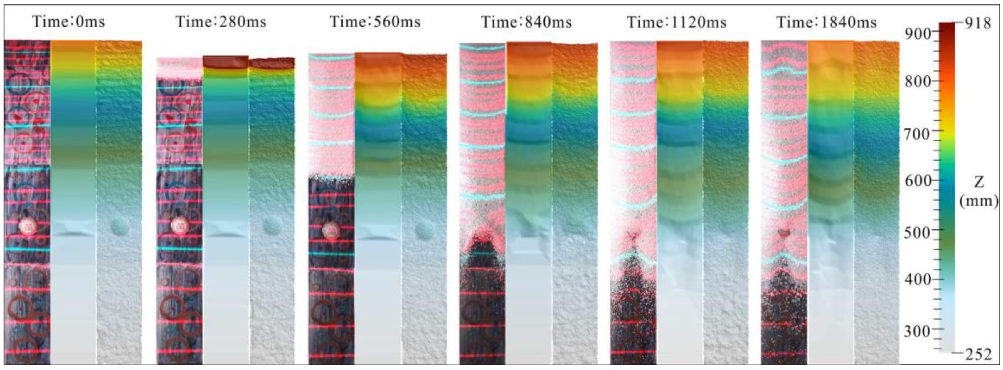
The movement path was significantly altered after the debris encountered a barrier at a high speed as the barrier of Experiment 5 was fixed in a high position. One part of debris crossed over the barrier and another part was divided into two groups and extruded on both sides (P5-4 and P5-6) of the barrier. The sampling probe (P5-7) in front of the barrier underwent complex changes during the experiment. This phenomenon can be interpreted as follows: the depth rapidly increased after the debris rapidly impacted the barrier, causing a “splash over” where a peak at approximately 540 ms was observed. Then, the shock effect of subsequent grains decreased gradually as the previous grains gradually accumulated; the depth gradually decreased after the peak depth. The movement behavior of the debris can be understood as the transitioning from “splashing over” to “climbing across”. At later time points in this experiment, the sampling probe gradually increased again when the entire barrier was completely submerged in debris. P5-8 is far from the barrier, meaning that it cannot be directly reached by the “splash over” at a given target velocity; therefore, the growth of the depth is a slow process. When the barrier is located at the slope toe (such as in Experiment 6), the “splashed over” movement patterns were difficult to observe at lower speeds. The sampling probes on the top of the spherical crown (P6-6) and its anterior (such as P6-8, P6-9) remain constant after reaching a relatively small numerical value.

5.3. Evolution of Depth

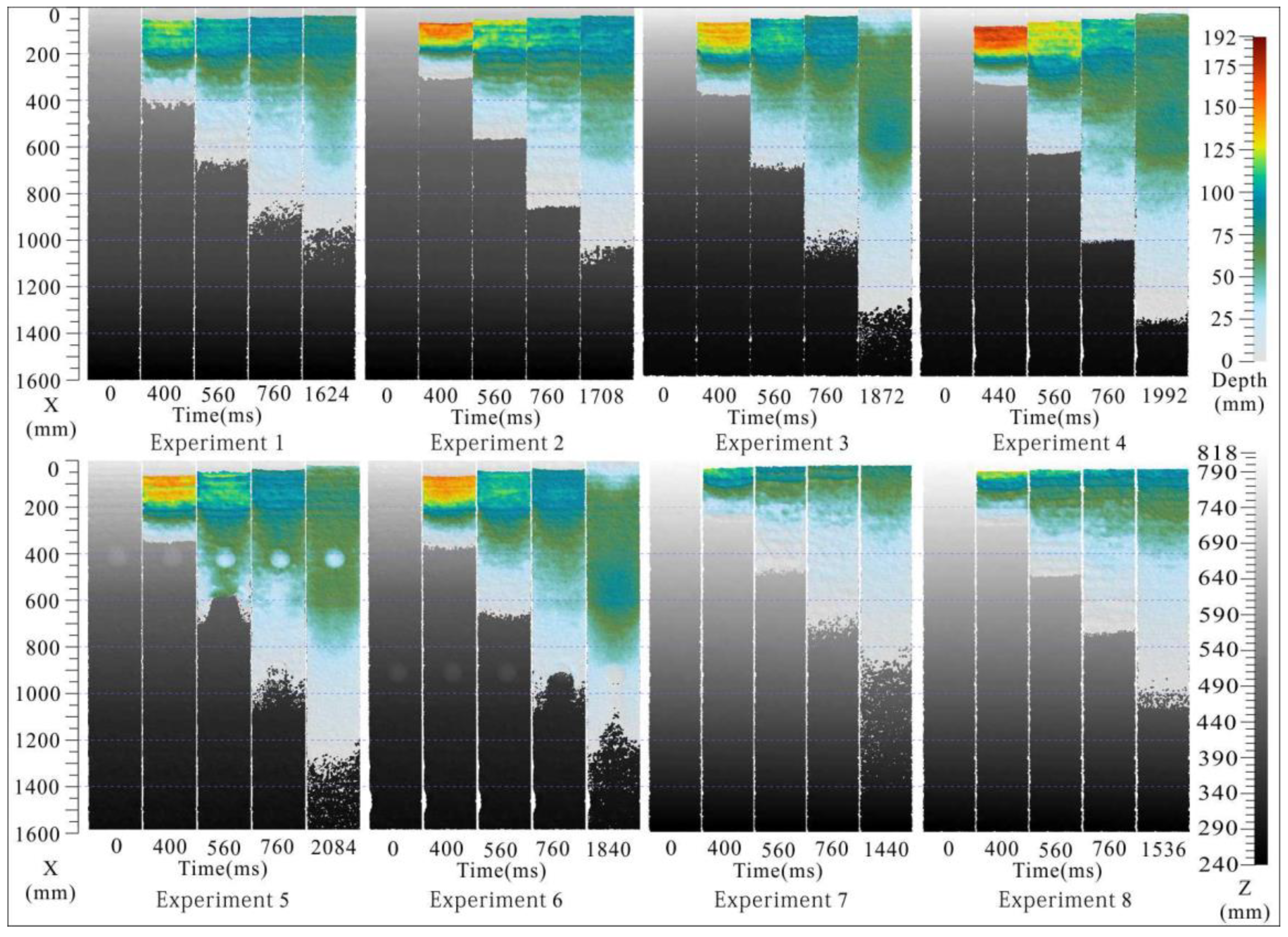
Similarly, the evolution of depth can also be obtained by a series of subtraction operations between the transient states and initial slope. Figure 14 not only visually illustrates the depth changing of every area but also presents the travel distance and deposit range; a number of interesting observations can be found through analyzing this map. The strongest correlation for the travel distance of debris is the slope shape. The travel distance of slope B (Experiments 4–6) was maximum and the result coincided with the evolution of volume. However, the travel distance of slope A was very close to the travel distance of slope C, which was significantly different from the evolution of volume (the volume of slope A > the volume of slope C). In the intermediate area, the depth of slope A was larger than the depth of slope C. These may be due to the different tilt angle at the first area, with the accelerating effect of slope A being bigger than that of slope C. There are significant differences in the depth distributions of these experiments. For example, the volume productivity in Experiments 3 and 6 was approximately 1.0, the depth distribution was high in the middle and low in the two ends as all the debris escaped the bin gate. However, the volume productivity in other experiments was less than 1.0 and the depth increased gradually from the forward end to the back end. These phenomena are closely related to the slope shape and replenishment of provenance. If the slope shape is in favor of the granular movement and the supply of provenance is not relatively abundant, the depth of the trailing debris will decrease to zero. The depth distribution was described as such in Experiments 3 and 6. If the above conditions are not satisfied, the depth distribution will look like the shape of other experiments. In addition, the position of the barrier has an impact on morphology distribution. When the barrier was located at the upper portion, the depth of the trailing debris was less than the control group or even zero. Correspondingly, the impact of the depth was rather limited when the barrier was located at the lower portion. Figure 14 displays rough temporal evolution among areas with different evolutionary histories. The intermediate area and leading area of the chute showed a gradual increase and the trailing area increased rapidly followed by a gradual decline. The details will be discussed in the following sections.

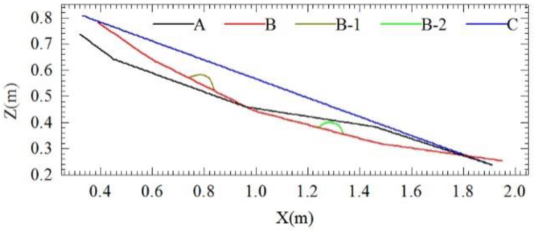
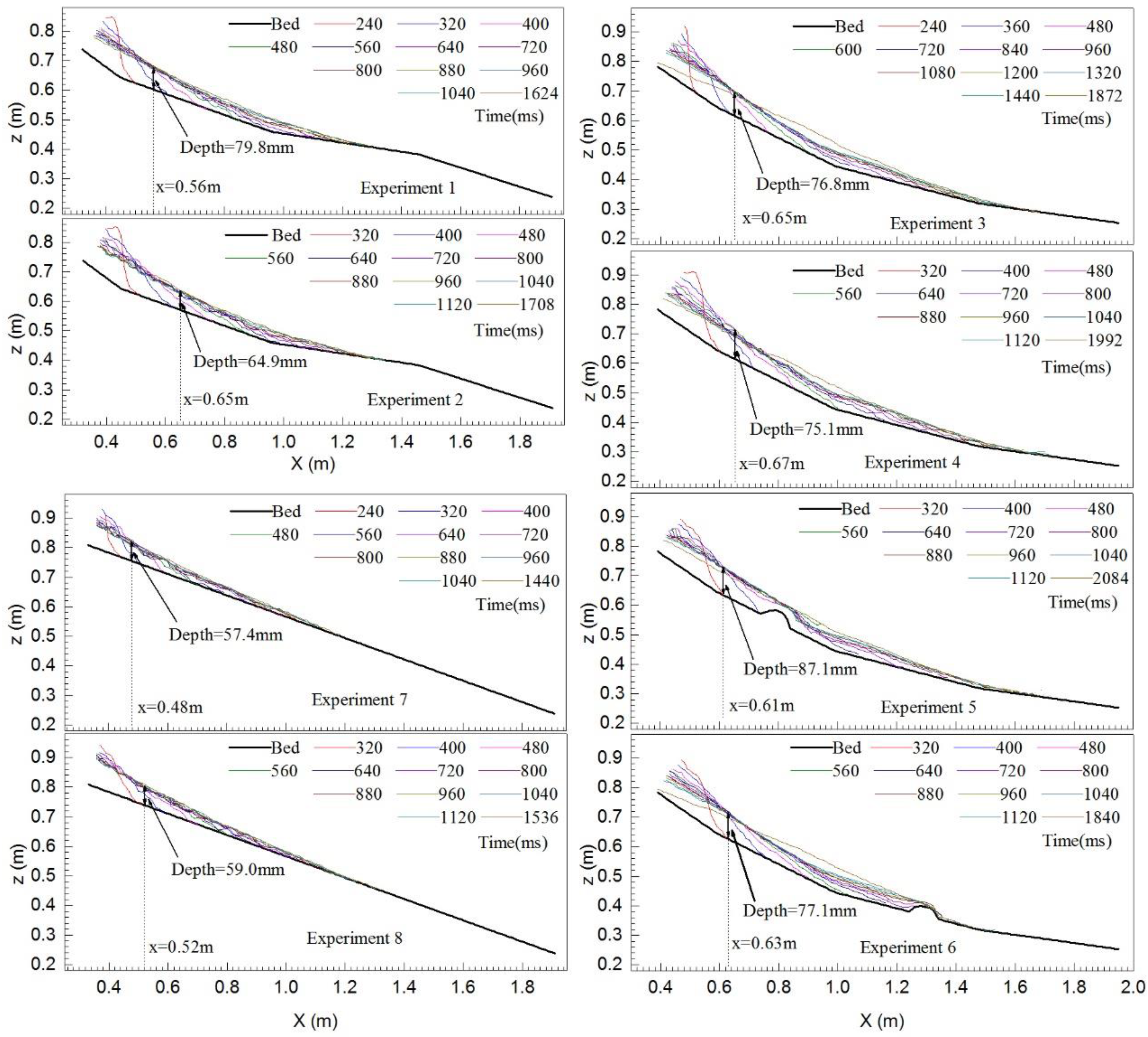
The time series of typical profiles are shown in Figure 15 from which the same conclusions can be drawn; i.e., the thickness of the intermediate and leading area increased gradually and the thickness of the trailing area first increased then decreased. Another observed phenomenon is that the travel distance of the debris increased rapidly in the early phase and gradually reached a steady state in the late phase. Another interesting finding is that there exists an intersection point for each profile lines in all the experimental groups. Once the maximum was achieved, the thickness remained constant. There were common intersection points for all the profile lines, where the first point to observe at which the thickness (or depth) of the debris remains constant after reaching its maximum was termed its “binding point”. Figure 15 shows the specific location for these points. The x-coordinate value of these points is dependent on the experimental conditions. For the slope shape, their sequence is slope B > slope A > slope C. The groups of quartz sand have a larger x-value than the control groups. Again, there is little adverse influence on the x-coordinate value in the experiment with the lower barrier. The ranking for the x-coordinate values is the same as those of the volume. That is, the larger volume, the larger the x-coordinate value of the binding point. To answer questions as to why and how this occurs, perhaps a more detailed analysis of energy conversion behavior, quantifying the collisions and interactions of the debris will be necessary. Due to space limitations, we will show these results in the follow-up work.

Although there were significant and striking differences for each group, this does not hinder the study of energy conversion behavior. For Experiment 3 (Figure 11, Figure 13 and Figure 15), the law of energy conversion in each stage is as follows: at the acceleration stage (0~500 ms), the depth and volume continuously increased with the enlargement of the range of deposit and the potential energy transformed into kinetic energy at a relatively high speed. At the constant stage (500~900 ms), when the “binding point” reached the steady-state, the volume growth rate remained relatively stable and the velocity of the debris remained approximately constant; the speed at which the potential energy transformed into kinetic energy was almost identical to the energy dissipation rate. At the deceleration stage (900~1872 ms), with the increase in travel distance, the volume changed at a slower rate by the gradual reduction of the locomotion speed. Deposition occurred in a stepwise pattern from front to back and the speed at which the potential energy transformed into kinetic energy was less than the energy dissipation rate. In this case, the slope shape favored the debris movement so that the depth of trailing debris decreased to zero; ultimately, the decreasing amount of potential energy equaled the energy dissipation.

6. Challenges and Perspectives

A total of eight experimental groups were designed to analyze the dynamic behavior and deposit features of avalanches, extensively covering the different combinations of granular size, slope angle, and barrier effect. However, many factors, such as granular material, size distribution, moisture content, granular size and shape, etc., affected the outcomes. Additionally, the experimental condition of equal volumes with different masses also significantly affected the outcomes. These factors are worthy of further study and exploration. In addition, specialized research for a series of experiments at different tilt angles could be designed to study the impact of slope angle. Similarly, this method can also be used to study the impact of granular size, size distribution, moisture content, etc. The method makes these issues more interpretable as it can provide abundant dynamic topographic data for experimental data analysis.

On the other hand, statistical analysis on these debris velocities has not been conducted in great detail due to the complexity of its problems. In future experiments, debris motion speed can be obtained by placing some tracer particles in the storage bin using the method described above. On this basis, it also can investigate the interaction strength between debris and understand the energy conversion mechanisms, usefully demystifying the movement law of this debris.

The 3D spatial data of dynamic scenes over time include point cloud data, DEM, mesh, texture, etc. As the main purpose of the study is to analyze the dynamic behavior of debris under various experimental conditions, this can be completed by post-processing the point cloud data. Certainly, other data can also be used in the analysis of these experiments for various research purposes. For example, reference data or a corrected model for numerical simulation based on mesh data and basic data of dynamic scenes for virtual reality (VR) obtained from texture data could be useful in widening the application fields for earth science researchers.

As expected, factors such as granular size, slope angle, and barrier effect are all influential for the dynamic behavior and deposit features of debris in these experiments. Specifically, the dynamic topographic data can be used to analyze travel distance and volume of debris avalanche. It is very significant in reducing the loss of life and property in mountain areas. For example, the management policies and measures in disaster mitigation can be established and implemented based on the geological condition (such as the granular size, slope angle, and barrier effect), which will contribute to sustainable development of economy and society in mountain areas. Thus, the vast amount of potentially new information regarding debris surface changes will undoubtedly lead us to more exciting applications.

7. Conclusions

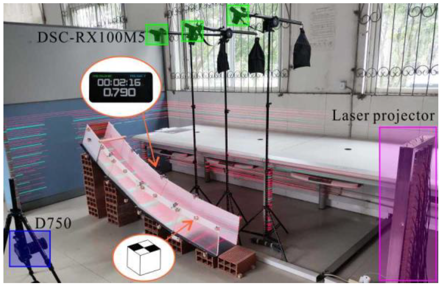
In this work, an approach to quantify surface changes of debris avalanche with high spatial and temporal resolution utilizing high-speed close-range photogrammetry is presented. Three DSC-RX100M5 digital cameras were used to acquire images in millisecond-range intervals. Based on these images, the 3D Spatial data of dynamic scenes were obtained accurately with the close-range photogrammetry. Compared with conventional image acquisition methods, more spatial information has been included in our research, acquiring more precise topographical data than the projected fringe method. Meanwhile, this method can be completed using a consumer-grade digital camera, which overcomes many of the shortcomings of traditional methods with low economic costs. The application of 4D reconstruction allows for the measurement of transient topographic data and monitoring of surface changes during experimentation. These data of surface changes include the temporal evolution of volume, evolution of depth, time-course curves of sampling probe, etc. After detailed analyses of these data, the following conclusions have been drawn: (1) the propagation and deposit processes of the debris avalanche have evident stage characteristics, which can be divided into the starting, acceleration, constant, and deceleration stages; (2) the granular size, slope angle, and barrier effect have a great influence on the travel distance and duration of the debris avalanche. (3) The depth of the intermediate and leading area of the debris avalanche increased gradually and the depth of the trailing area first increased then decreased. We believe that this approach can be used for other model tests involving the acquisition of dynamic terrain data. Therefore, the technique has broad application prospects in model tests.

References

1. Xu, Q.; Li, H.; He, Y.; Liu, F.; Peng, D. Comparison of data-driven models of loess landslide runout distance estimation. Bull. Eng. Geol. Environ. 2019, 78, 1281–1294. [Google Scholar] [CrossRef]
2. Pastor-Escuredo, D.; Torres, Y.; Martínez-Torres, M.; Zufiria, P.J. Rapid Multi-Dimensional Impact Assessment of Floods. Sustainability 2020, 12, 4246. [Google Scholar] [CrossRef]
3. Hu, W.; Scaringi, G.; Xu, Q.; Huang, R. Internal erosion controls failure and runout of loose granular deposits: Evidence from flume tests and implications for postseismic slope healing. Geophys. Res. Lett. 2018, 45, 5518–5527. [Google Scholar] [CrossRef]
4. Xu, Q.; Liu, H.; Ran, J.; Li, W.; Sun, X. Field monitoring of groundwater responses to heavy rainfalls and the early warning of the Kualiangzi landslide in Sichuan Basin, southwestern China. Landslides 2016, 13, 1555–1570. [Google Scholar] [CrossRef]
5. Wang, Z.; Huang, N. Numerical simulation of the falling snow deposition over complex terrain. J. Geophys. Res. Atmos. 2017, 122, 980–1000. [Google Scholar] [CrossRef]
6. Jiang, Y.; Li, B.; Yamashita, Y. Simulation of cracking near a large underground cavern in a discontinuous rock mass using the expanded distinct element method. Int. J. Rock Mech. Min. Sci. 2009, 46, 97–106. [Google Scholar] [CrossRef] [Green Version]
7. Caballero, L.; Sarocchi, D.; Borselli, L.; Cárdenas, A.I. Particle interaction inside debris flows: Evidence through experimental data and quantitative clast shape analysis. J. Volcanol. Geotherm. Res. 2012, 231, 12–23. [Google Scholar] [CrossRef]
8. Kaitna, R.; Palucis, M.C.; Yohannes, B.; Hill, K.M.; Dietrich, W.E. Effects of coarse grain size distribution and fine particle content on pore fluid pressure and shear behavior in experimental debris flows. J. Geophys. Res. Earth Surf. 2016, 121, 415–441. [Google Scholar] [CrossRef] [Green Version]
9. Cui, S.; Pei, X.; Wu, H.; Huang, R. Centrifuge model test of an irrigation-induced loess landslide in the Heifangtai loess platform, Northwest China. J. Mt. Sci. 2018, 15, 130–143. [Google Scholar] [CrossRef]
10. Lü, X.; Xue, D.; Chen, Q.; Zhai, X.; Huang, M. Centrifuge model test and limit equilibrium analysis of the stability of municipal solid waste slopes. Bull. Eng. Geol. Environ. 2019, 78, 3011–3021. [Google Scholar] [CrossRef]
11. Miao, F.; Wu, Y.; Li, L.; Tang, H.; Li, Y. Centrifuge model test on the retrogressive landslide subjected to reservoir water level fluctuation. Eng. Geol. 2018, 245, 169–179. [Google Scholar] [CrossRef]
12. Li, S.; Xu, Q.; Tang, M.; Li, H.; Yang, H.; Wei, Y. Centrifuge Modeling and the Analysis of Ancient Landslides Subjected to Reservoir Water Level Fluctuation. Sustainability 2020, 12, 2092. [Google Scholar] [CrossRef] [Green Version]
13. De Haas, T.; Braat, L.; Leuven, J.R.; Lokhorst, I.R.; Kleinhans, M. Effects of debris flow composition on runout, depositional mechanisms, and deposit morphology in laboratory experiments. J. Geophys. Res. Earth Surf. 2015, 120, 1949–1972. [Google Scholar] [CrossRef] [Green Version]
14. Zhou, G.G.; Li, S.; Song, D.; Choi, C.E.; Chen, X. Depositional mechanisms and morphology of debris flow: Physical modelling. Landslides 2019, 16, 315–332. [Google Scholar] [CrossRef]
15. Wang, Y.; Zhang, D.; Hu, Y. Laboratory investigation of the effect of injection rate on hydraulic fracturing performance in artificial transversely laminated rock using 3D laser scanning. Geotech. Geol. Eng. 2019, 37, 2121–2133. [Google Scholar] [CrossRef]
16. Zhang, B.; Wang, H.; Huang, J.; Xu, N. Model test on slope deformation and failure caused by transition from open-pit to underground mining. Geomech. Eng. 2019, 19, 167–178. [Google Scholar]
17. Robbersmyr, K.G.; Gåsvik, K.J.; Vadseth, T.; Karimi, H.R. Surface topography measurement of double-curved propeller blades using projected fringes. Int. J. Adv. Manuf. Technol. 2017, 91, 375–381. [Google Scholar] [CrossRef]
18. Iverson, R.M.; Logan, M.; Denlinger, R.P. Granular avalanches across irregular three-dimensional terrain: 2. Experimental tests. J. Geophys. Res. Earth Surf. 2004, 109. [Google Scholar] [CrossRef]
19. Caviedes-Voullième, D.; Juez, C.; Murillo, J.; García-Navarro, P. 2D dry granular free-surface flow over complex topography with obstacles. Part I: Experimental study using a consumer-grade RGB-D sensor. Comput. Geosci. 2014, 73, 177–197. [Google Scholar] [CrossRef]
20. Luhmann, T. Close range photogrammetry for industrial applications. ISPRS J. Photogramm. Remote Sens. 2010, 65, 58–569. [Google Scholar] [CrossRef]
21. Luis, P.; Tomás, M.; Vicente, B.; Alejandro, J.S. Photogrammetric studies of inaccessible sites in archaeology: Case study of burial chambers in Qubbet el-Hawa (Aswan, Egypt). J. Archaeol. Sci. 2019, 102, 1–10. [Google Scholar] [CrossRef]
22. Rodríguez-Gonzálvez, P.; Mancera-Taboada, J.; González-Aguilera, D.; Muñoz-Nieto, Á.; Armesto, J.A. hybrid approach to create an archaeological visualization system for a Palaeolithic cave. Archaeometry 2012, 54, 565–580. [Google Scholar] [CrossRef]
23. Jo, Y.H.; Hong, S. Three-dimensional digital documentation of cultural heritage site based on the convergence of terrestrial laser scanning and unmanned aerial vehicle photogrammetry. ISPRS Int. J. Geo-Inf. 2019, 8, 53. [Google Scholar] [CrossRef] [Green Version]
24. Fritsch, D.; Klein, M. 3D preservation of buildings–reconstructing the past. Multimed. Tools Appl. 2018, 77, 9153–9170. [Google Scholar] [CrossRef]
25. Li, W.; Bertin, S.; Friedrich, H. Combining Structure from Motion and close-range stereo photogrammetry to obtain scaled gravel bar DEMs. Int. J. Remote Sens. 2018, 39, 9269–9293. [Google Scholar] [CrossRef]
26. Smith, M.; Carrivick, J.; Quincey, D. Structure from motion photogrammetry in physical geography. Prog. Phys. Geogr. 2016, 40, 247–275. [Google Scholar] [CrossRef]
27. Alameda-Hernández, P.; El Hamdouni, R.; Irigaray, C.; Chacón, J. Weak foliated rock slope stability analysis with ultra-close-range terrestrial digital photogrammetry. Bull. Eng. Geol. Environ. 2019, 78, 1157–1171. [Google Scholar] [CrossRef]
28. Janowski, A.; Szulwic, J.; Ziółkowski, P. Combined method of surface flow measurement using terrestrial laser scanning and synchronous photogrammetry. In 2017 Baltic Geodetic Congress (BGC Geomatics); IEEE: Gdansk, Poland, 2017; pp. 110–115. [Google Scholar]
29. Baqersad, J.; Poozesh, P.; Niezrecki, C.; Avitabile, P. Photogrammetry and optical methods in structural dynamics–A review. Mech. Syst. Signal Process. 2017, 86, 17–34. [Google Scholar] [CrossRef]
30. Poozesh, P.; Baqersad, J.; Niezrecki, C.; Avitabile, P.; Harvey, E.; Yarala, R. Large-area photogrammetry based testing of wind turbine blades. Mech. Syst. Signal Process. 2017, 86, 98–115. [Google Scholar] [CrossRef] [Green Version]
31. Poozesh, P.; Sarrafi, A.; Mao, Z.; Avitabile, P.; Niezrecki, C. Feasibility of extracting operating shapes using phase-based motion magnification technique and stereo-photogrammetry. J. Sound Vib. 2017, 407, 350–366. [Google Scholar] [CrossRef]
32. Havaran, A.; Mahmoudi, M. Extracting structural dynamic properties utilizing close photogrammetry method. Measurement 2020. [Google Scholar] [CrossRef]
33. Tong, X.; Gao, S.; Liu, S.; Ye, Z.; Chen, P. Monitoring a progressive collapse test of a spherical lattice shell using high-speed videogrammetry. Photogramm. Rec. 2017, 32, 230–254. [Google Scholar] [CrossRef]
34. Cheluszka, P.; Mann, R. Vibration identification of the roadheader cutting head using high-speed cameras. MATEC Web Conf. 2019, 252, 03018. [Google Scholar] [CrossRef] [Green Version]
35. James, M.; Robson, S. Sequential digital elevation models of active lava flows from ground-based stereo time-lapse imagery. ISPRS J. Photogramm. Remote Sens. 2014, 97, 160–170. [Google Scholar] [CrossRef]
36. Eltner, A.; Kaiser, A.; Abellan, A.; Schindewolf, M. Time lapse structure-from-motion photogrammetry for continuous geomorphic monitoring. Earth Surf. Process. Landf. 2017, 42, 2240–2253. [Google Scholar] [CrossRef]
37. Guo, M.; Shi, H.; Zhao, J.; Liu, P.; Welbourne, D. Digital close range photogrammetry for the study of rill development at flume scale. Catena 2016, 143, 265–274. [Google Scholar] [CrossRef]
38. Jiang, Y.; Shi, H.; Wen, Z.; Guo, M.; Zhao, J. The dynamic process of slope rill erosion analyzed with a digital close range photogrammetry observation system under laboratory conditions. Geomorphology 2020. [Google Scholar] [CrossRef]
39. Scaioni, M.; Feng, T.; Barazzetti, L.; Previtali, M.; Lu, P. Some applications of 2-D and 3-D photogrammetry during laboratory experiments for hydrogeological risk assessment. Geomat. Nat. Hazards Risk 2015, 6, 473–496. [Google Scholar] [CrossRef] [Green Version]
40. Huang, S.; Zhang, Z.; Zhao, Y.; Dai, J.; Chen, C. 3D fingerprint imaging system based on full-field fringe projection profilometry. Opt. Lasers Eng. 2014, 52, 123–130. [Google Scholar] [CrossRef]
41. Zhang, S. Recent progresses on real-time 3D shape measurement using digital fringe projection techniques. Opt. Lasers Eng. 2010, 48, 149–158. [Google Scholar] [CrossRef]
42. Thielicke, W.; Stamhuis, E. PIVlab-towards user-friendly, affordable and accurate digital particle image velocimetry in MATLAB. J. Open Res. Softw. 2014, 2, 1–10. [Google Scholar] [CrossRef] [Green Version]
Figure 1. Perspective view of the chute which may be set to any desired angle through U-shaped clips and hinges.
Sustainability 12 06578 g001
Figure 2. Visual perspective of the experimental facility.
Sustainability 12 06578 g002
Figure 3. Granular diameter: (a) polished gravel and (b) quartz sand.
Sustainability 12 06578 g003
Figure 4. Chute slope profiles.
Sustainability 12 06578 g004
Figure 5. Data acquisition and processing workflow.
Sustainability 12 06578 g005
Figure 6. Actual work images: (a) slow motion video from RX100M5 cameras, (b) extract frames from slow motion video, (c) the interface of Agisoft Metashape, and (d) 3D spatial sequence data.
Sustainability 12 06578 g006
Figure 7. 3D spatial data of Experiment 6 at 840 ms. (a) Panoramic data of original data; the local magnified data of (a): (b) point cloud data, (c) mesh data, and (d) texture data.
Sustainability 12 06578 g007
Figure 8. Residual level: (a) R1 residual error, (b) R2 residual error, and (c) R3 residual error.
Sustainability 12 06578 g008
Figure 9. Projected fringe method data capture method.
Sustainability 12 06578 g009
Figure 10. Data comparison, which are, from left to the right, image data, fringe projection digital elevation model (DEM) data, and photogrammetric DEM data.
Sustainability 12 06578 g010
Figure 11. Temporal evolution. (a) Time-history curves of volume, (b) time-history curves of volume productivity (the ratio of the outlet gate volume to the initial volume).
Sustainability 12 06578 g011
Figure 12. Sampling probe locations.
Sustainability 12 06578 g012
Figure 13. Time-history curves of sampling probe. The location of these sampling points is shown in Figure 12. The depth of the debris is the vertical distance from the sampling point to the bottom surface of the chute.
Sustainability 12 06578 g013
Figure 14. Depth evolution. The figure shows bed elevation in grayscale and sand depth in colors. X-values correspond to the coordinate of the 4D model, and the values in x direction were set to zero.
Sustainability 12 06578 g014
Figure 15. Evolution of typical profile (longitudinal section of the debris surfaces along the X-axis.). The bottom surfaces (beds) of the chute are represented by thick black lines, and the debris surfaces at different times are indicated with colored lines.
Sustainability 12 06578 g015