Hazard-Consistent Earthquake Scenario Selection for Seismic Slope Stability Assessment


Abstract
:1. Introduction
2. Materials and Methods
2.1. Method
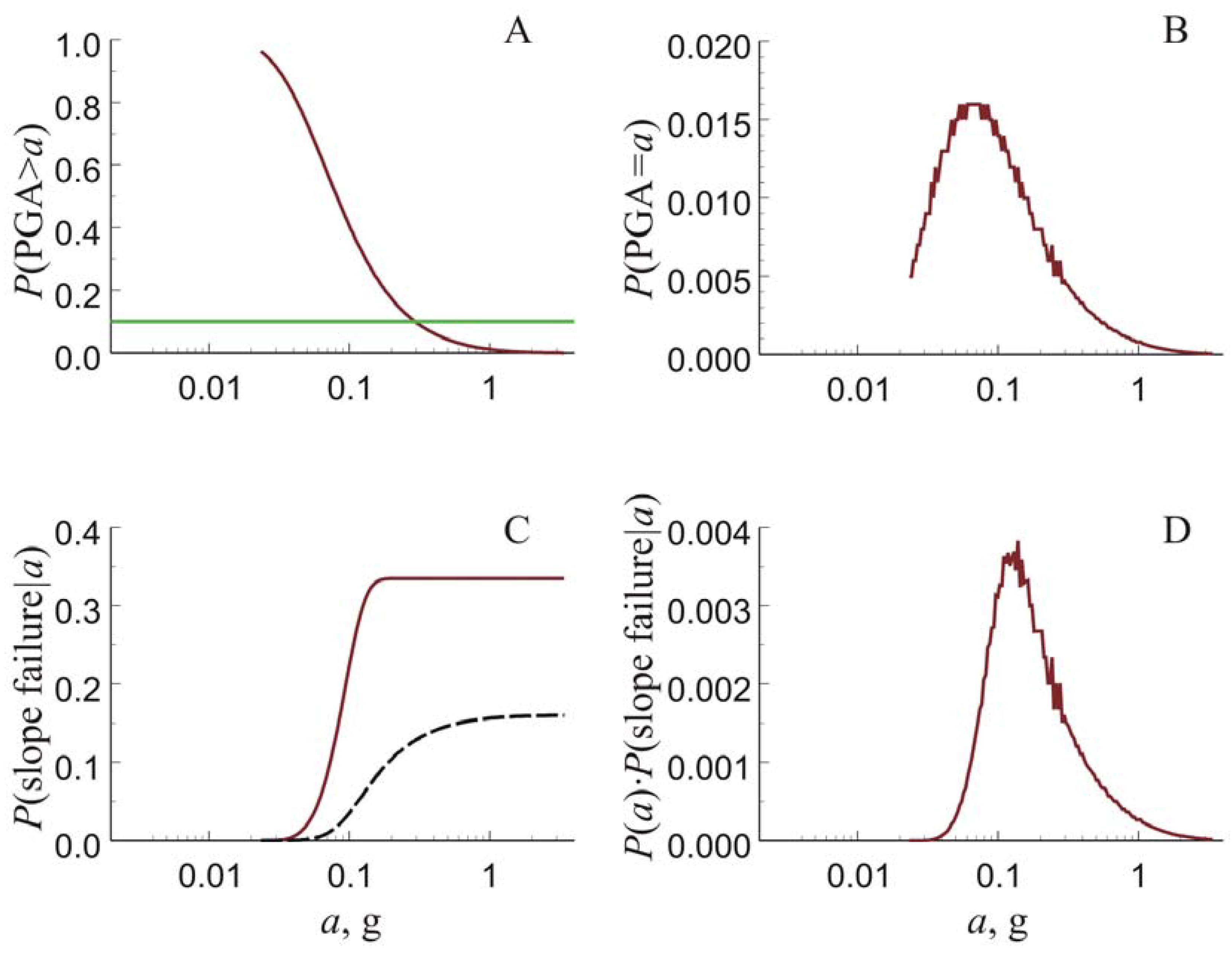
2.1.1. Fully Probabilistic Approach
2.1.2. Conditional Probability of Slope Failure Under Seismic Loading
2.1.3. Probability of Occurrence of Ground Shaking Intensity
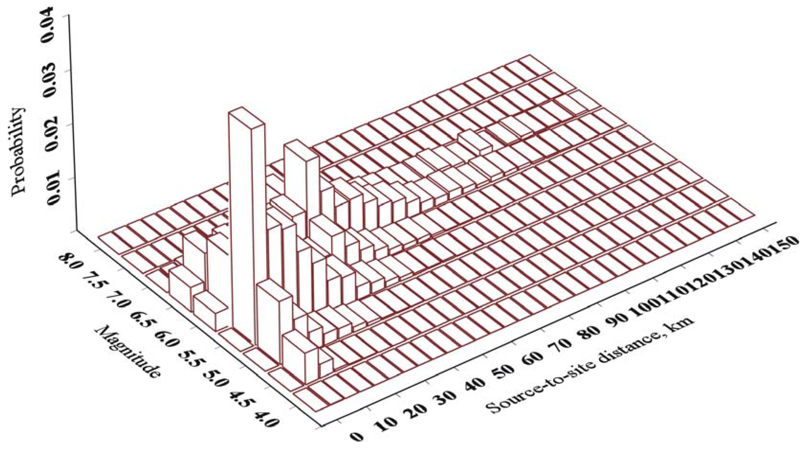
2.1.4. Occurrence Hazard Deaggregation
2.2. Materials
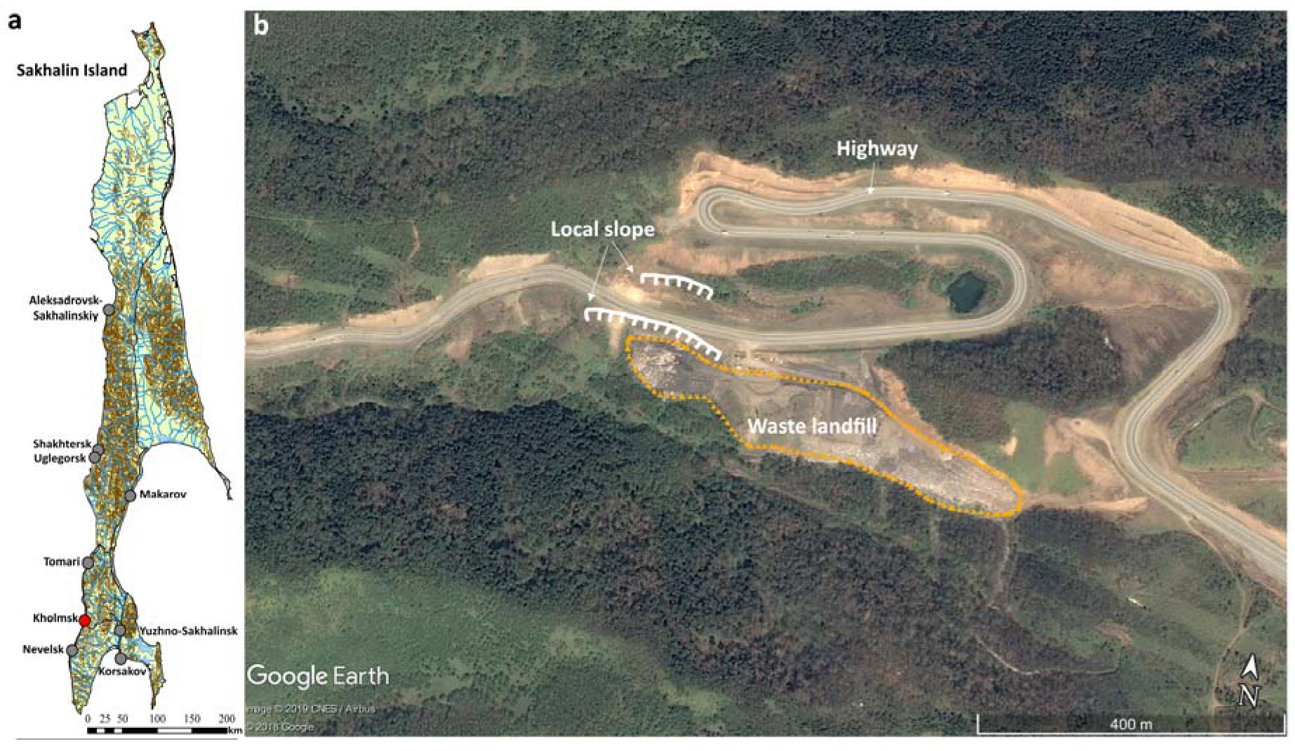
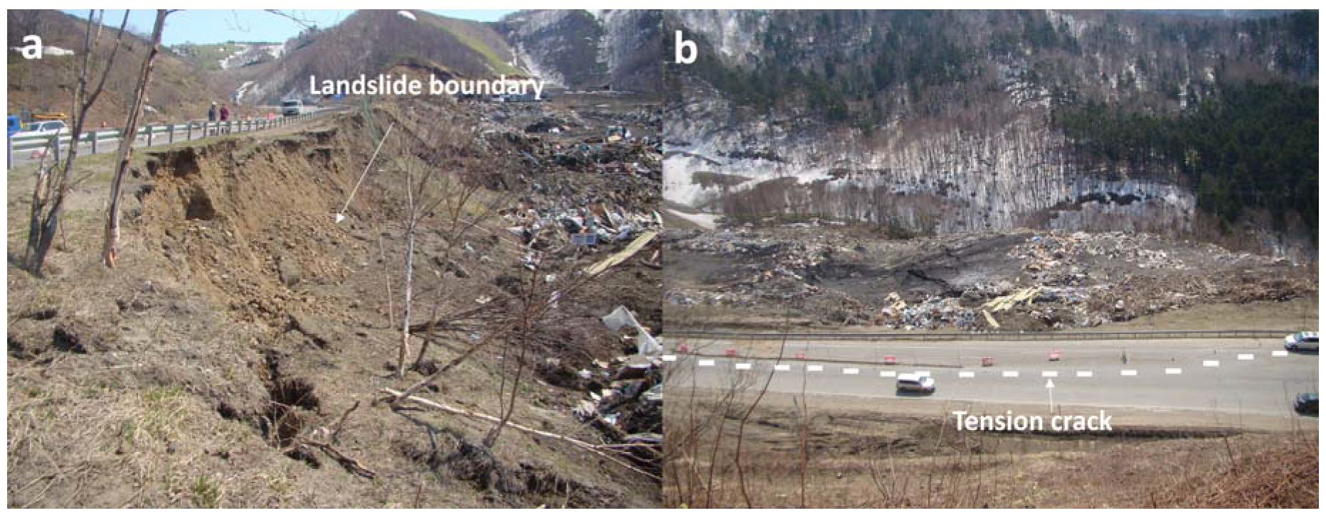
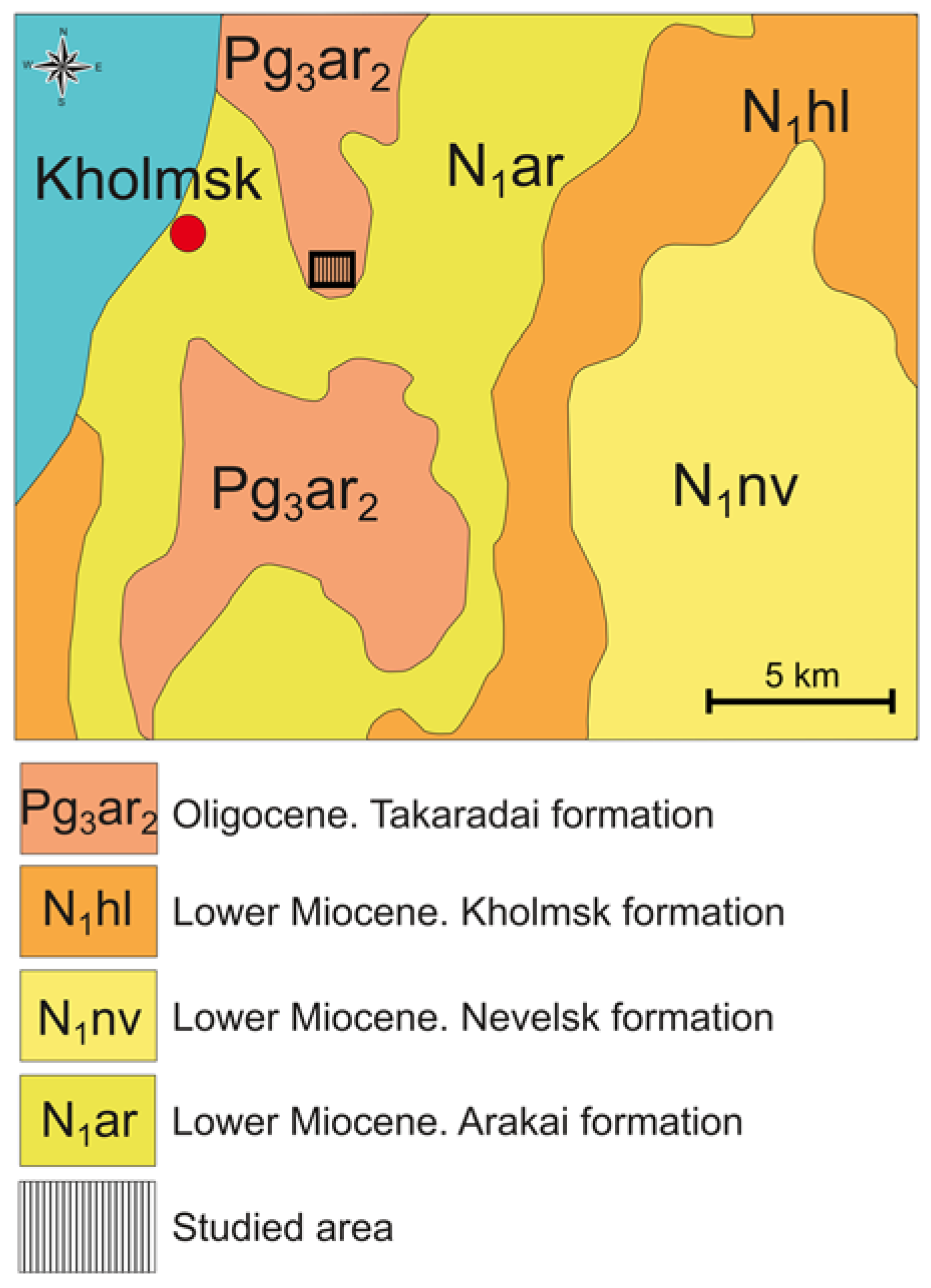
2.2.1. Studied Area
2.2.2. Geomechanical Slope Model
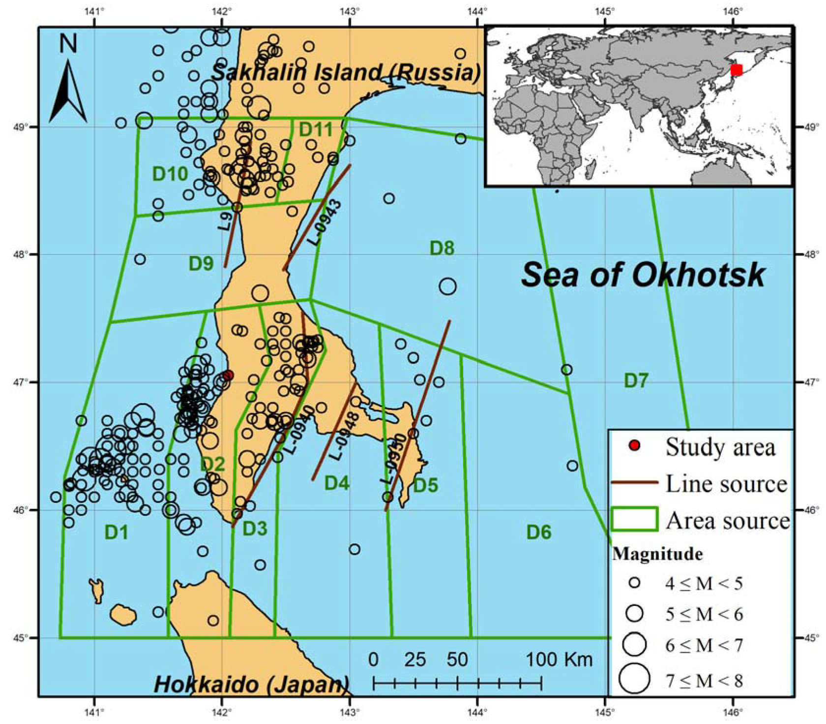
2.2.3. Seismic Source Model and GMPEs
3. Results
4. Discussion
5. Conclusions
Author Contributions
Funding
Conflicts of Interest
References
- Jibson, R.W. Methods for assessing the stability of slopes during earthquakes–A retrospective. Eng. Geol. 2011, 122, 43–50. [Google Scholar] [CrossRef]
- Fabbri, A.G.; Chung, C.-J.F.; Cendrero, A.; Remondo, J. Is Prediction of Future Landslides Possible with a GIS? Nat. Hazards 2003, 30, 487–503. [Google Scholar] [CrossRef]
- Jibson, R.W.; Michael, J.A. Maps Showing Seismic Landslide Hazards in Anchorage, Alaska: U.S. Geological Survey Scientific Investigations Map 3077, Scale 1:25,000, 11-p. Pamphlet. 2009. Available online: http://pubs.usgs.gov/sim/3077 (accessed on 18 March 2019).
- Lee, C.T.; Huang, C.C.; Lee, J.F.; Pan, K.L.; Lin, M.L.; Dong, J.J. Statistical approach to earthquake-induced landslide susceptibility. Eng. Geol. 2008, 100, 43–58. [Google Scholar] [CrossRef]
- Jibson, R.W.; Harp, E.L.; Michael, J.A. A Method for Producing Digital Probabilistic Seismic Landslide Hazard Maps: An Example from Southern CALIFORNIA; Open-File Report 98-113; U.S. Geological Survey: Reston, VA, USA, 1998. Available online: https://pubs.usgs.gov/of/1998/ofr-98-113/ofr-98-113.pdf (accessed on 18 March 2019).
- Lee, C.T. Statistical seismic landslide hazard analysis: An example from Taiwan. Eng. Geol. 2014, 182, 201–212. [Google Scholar] [CrossRef]
- Pareek, N.; Pal, S.; Kaynia, A.M.; Sharma, M.L. Empirical-based seismically induced slope displacements in a geographic information system environment: A case study. Georisk Assess. Manag. Risk Eng. Syst. Geohazards 2015, 8, 258–268. [Google Scholar] [CrossRef]
- Keefer, D.K. Statistical analysis of an earthquake-induced landslide distribution—The 1989 Loma Prieta, California event. Eng. Geol. 2000, 58, 231–249. [Google Scholar] [CrossRef]
- Jibson, R.W.; Harp, E.L.; Michael, J.A. A method for producing digital probabilistic seismic landslide hazard maps. Eng. Geol. 2000, 58, 271–289. [Google Scholar] [CrossRef]
- Jibson, R.W. Mapping seismic landslide hazards in Anchorage, Alaska. In Proceedings of the 10th National Conference in Earthquake Engineering, Earthquake Engineering Research Institute, Anchorage, AK, USA, 21–25 July 2014. [Google Scholar]
- Wang, T.; Liu, J.; Shi, J.; Wu, S. The influence of DEM resolution on seismic landslide hazard assessment based upon the Newmark displacement method: A case study in the loess area of Tianshui, China. Environ. Earth Sci. 2017, 76, 604. [Google Scholar] [CrossRef]
- Rathje, E.M.; Saygili, G. Estimating Fully Probabilistic Seismic Sliding Displacements of Slopes from a Pseudoprobabilistic Approach. J. Geotech. Geoenviron. Eng. 2011, 137, 208–217. [Google Scholar] [CrossRef]
- Magrin, A.; Peresan, A.; Kronrod, T.; Vaccari, F.; Panza, G.F. Neo-deterministic seismic hazard assessment and earthquake occurrence rate. Eng. Geol. 2017, 229, 95–109. [Google Scholar] [CrossRef]
- Bojadjieva, J.; Sheshov, V.; Bonnard, C. Hazard and risk assessment of earthquake-induced landslides—Case study. Landslides 2018, 15, 161–171. [Google Scholar] [CrossRef]
- Rathje, E.M.; Saygili, G. Probabilistic Seismic Hazard Analysis for the Sliding Displacement of Slopes: Scalar and Vector Approaches. J. Geotech. Geoenviron. Eng. 2008, 134, 804–814. [Google Scholar] [CrossRef]
- Martino, S.; Battaglia, S.; Delgado, J.; Esposito, C.; Martini, G.; Missori, C. Probabilistic Approach to Provide Scenarios of Earthquake-Induced Slope Failures (PARSIFAL) Applied to the Alcoy Basin (South Spain). Geosciences 2018, 8, 57. [Google Scholar] [CrossRef] [Green Version]
- Martino, S.; Battaglia, S.; D’Alessandro, F.; Della Seta, M.; Esposito, C.; Martini, G.; Pallone, F.; Troiani, F. Earthquake-induced landslide scenarios for seismic microzonation: Application to the Accumoli area (Rieti, Italy). Bull. Earthq. Eng. 2019, 1–19. [Google Scholar] [CrossRef] [Green Version]
- Del Gaudio, V.; Wasowski, J.; Pierri, P. An Approach to Time-Probabilistic Evaluation of Seismically Induced Landslide Hazard. Bull. Seismol. Soc. Am. 2003, 93, 557–569. [Google Scholar] [CrossRef]
- Olsen, M.J.; Ashford, S.A.; Mahlingam, R.; Sharifi-Mood, M.; O’Banion, M.; Gillins, D.T. Impacts of Potential Seismic Landslides on Lifeline Corridors; Final Report SPR 740; School of Civil and Construction Engineering Oregon State University: Corvallis, OR, USA, 2015; p. 240. [Google Scholar]
- Refice, A.; Capolongo, D. Probabilistic Modeling of Uncertainties in Earthquake-Induced Landslide Hazard Assessment. Comput. Geosci. 2002, 28, 735–749. [Google Scholar] [CrossRef]
- Grünthal, G.; Stromeyer, D.; Bosse, C.; Cotton, F.; Bindi, D. The probabilistic seismic hazard assessment of Germany—Version 2016, considering the range of epistemic uncertainties and aleatory variability. Bull. Earthq. Eng. 2018, 16, 4339–4395. [Google Scholar] [CrossRef] [Green Version]
- Earthquake Catalogue. Available online: https://eqalert.ru/#/events?datetime_min=1905-01-01%2000%3A00%3A00&depth_max=50&mag_min=4&lat_max=50&lat_min=45&lon_max=145&lon_min=140 (accessed on 20 May 2020).
- Konovalov, A.; Gensiorovskiy, Y.; Lobkina, V.; Muzychenko, A.; Stepnova, Y.; Muzychenko, L.; Stepnov, A.; Mikhalyov, M. Earthquake-Induced Landslide Risk Assessment: An Example from Sakhalin Island, Russia. Geosciences 2019, 9, 305. [Google Scholar] [CrossRef] [Green Version]
- Newmark, N.M. Effects of earthquakes on dams and embankments. Geotechnique 1965, 15, 139–159. [Google Scholar] [CrossRef] [Green Version]
- Wang, T.; Wu, S.R.; Shi, J.S.; Xin, P.; Wu, L.Z. Assessment of the effects of historical strong earthquakes on large-scale landslide groupings in the Wei River midstream. Eng. Geol. 2018, 235, 11–19. [Google Scholar] [CrossRef]
- Jibson, R.W. Regression models for estimating coseismic landslide displacement. Eng. Geol. 2007, 91, 209–218. [Google Scholar] [CrossRef]
- Romeo, R. Seismically induced landslide displacements: A predictive model. Eng. Geol. 2000, 58, 337–351. [Google Scholar] [CrossRef]
- Cornell, C.A. Engineering seismic risk analysis. Bull. Seismol. Soc. Am. 1968, 58, 1583–1606. [Google Scholar]
- Baker, J.W. Probabilistic Seismic Hazard Analysis; White Paper Version 2.0.1; Stanford University: Stanford, CA, USA, 2013; p. 79. [Google Scholar]
- Fox, M.J.; Stafford, P.J.; Sullivan, T.J. Seismic hazard disaggregation in performance-based earthquake engineering: Occurrence or exceedance? Earthq. Eng. Struct. Dynam. 2016, 45, 835–842. [Google Scholar] [CrossRef] [Green Version]
- Komsomolskiy, G.V.; Siryk, I.M. (Eds.) Atlas of the Sakhalin Region; GUGK Sovmin USSR: Moscow, Russia, 1967; p. 137. (In Russian) [Google Scholar]
- Sergeev, E.M. (Ed.) Engineering Geology of USSR; Far East; Lomonosov Moscow State University: Moscow, Russia, 1977; pp. 392–413. (In Russian) [Google Scholar]
- Levin, B.W.; Kim, C.U.; Solovjev, V.N. A seismic hazard assessment and the results of detailed seismic zoning for urban territories of Sakhalin Island. Russ. J. Pac. Geol. 2013, 7, 455–464. [Google Scholar] [CrossRef]
- Ulomov, V.I.; Bogdanov, M.I. Explanatory note on the GSZ-2016 maps set of general seismic zoning of the Russian Federation territory. Eng. Surv. 2016, 7, 49–122. (In Russian) [Google Scholar]
- Konovalov, A.V.; Sychov, A.S.; Manaychev, K.A.; Stepnov, A.A.; Gavrilov, A.V. Testing of a New GMPE Model in Probabilistic Seismic Hazard Analysis for the Sakhalin Region. Seism. Instr. 2019, 55, 283–290. [Google Scholar] [CrossRef]
- Abrahamson, N.A.; Silva, W.J.; Kamai, R. Summary of the ASK14 ground motion relation for active crustal regions. Earthq. Spectra 2014, 30, 1025–1055. [Google Scholar] [CrossRef]
- Aguilar-Meléndez, A.; Ordaz Schroeder, M.G.; De la Puente, J.; Gonzalez Rocha, S.N.; Rodrigez Lozoya, H.E.; Cordova Ceballos, A.; Garcia Elias, A.; Calderon Ramon, C.M.; Escalante Martinez, J.E.; Laguna Camacho, J.R.; et al. Development and Validation of Software CRISIS to Perform Probabilistic Seismic Hazard Assessment with Emphasis on the Recent CRISIS2015. Comput. Sist. 2017, 21, 67–90. [Google Scholar] [CrossRef]
- Burgess, J.; Fenton, G.A.; Griffiths, D.V. Probabilistic seismic slope stability analysis and design. Can. Geotech. J. 2019, 56, 1979–1998. [Google Scholar] [CrossRef] [Green Version]


| Soil type | , kpa | , m | , deg | , kN/m3 | , deg | ||
|---|---|---|---|---|---|---|---|
| Siltstone | 15.4 | 5.7 | 23 | 22 | 9.8 | 29.7 | 1 |
| Seismic Source | Annual Rate of Earthquakes with Magnitude Greater than | Value | Minimum Magnitude | Maximum Magnitude | Source Mechanism |
|---|---|---|---|---|---|
| D1 | 0.759 | 0.840 | 4.0 | 7.5 | Reverse |
| D2 | 0.794 | 1.000 | 4.0 | 7.0 | Reverse |
| D3 | 0.813 | 0.970 | 4.0 | 6.0 | Reverse |
| D4 | 0.427 | 1.110 | 4.0 | 5.5 | Reverse |
| D5 | 0.229 | 0.680 | 4.0 | 5.5 | Reverse |
| D7 | 0.151 | 0.730 | 4.0 | 5.7 | Reverse |
| D8 | 0.282 | 1.040 | 4.0 | 5.7 | Reverse |
| D9 | 0.204 | 1.340 | 4.0 | 5.5 | Reverse |
| D10 | 1.622 | 0.900 | 4.0 | 6.0 | Reverse |
| D11 | 0.447 | 0.710 | 4.0 | 6.0 | Reverse |
| L-0948 | 0.007 | 1.110 | 5.6 | 6.0 | Reverse |
| L-0940 | 0.007 | 0.970 | 6.1 | 7.5 | Reverse |
| L-0950 | 0.019 | 0.680 | 5.6 | 6.0 | Reverse |
| L-0943 | 0.001 | 1.340 | 5.6 | 6.5 | Reverse |
| L9 | >0.001 | >1.340 | >5.6 | >7.0 | >Reverse |
© 2020 by the authors. Licensee MDPI, Basel, Switzerland. This article is an open access article distributed under the terms and conditions of the Creative Commons Attribution (CC BY) license (http://creativecommons.org/licenses/by/4.0/).
Share and Cite
Konovalov, A.; Gensiorovskiy, Y.; Stepnov, A. Hazard-Consistent Earthquake Scenario Selection for Seismic Slope Stability Assessment. Sustainability 2020, 12, 4977. https://doi.org/10.3390/su12124977
Konovalov A, Gensiorovskiy Y, Stepnov A. Hazard-Consistent Earthquake Scenario Selection for Seismic Slope Stability Assessment. Sustainability. 2020; 12(12):4977. https://doi.org/10.3390/su12124977
Chicago/Turabian StyleKonovalov, Alexey, Yuriy Gensiorovskiy, and Andrey Stepnov. 2020. "Hazard-Consistent Earthquake Scenario Selection for Seismic Slope Stability Assessment" Sustainability 12, no. 12: 4977. https://doi.org/10.3390/su12124977
APA StyleKonovalov, A., Gensiorovskiy, Y., & Stepnov, A. (2020). Hazard-Consistent Earthquake Scenario Selection for Seismic Slope Stability Assessment. Sustainability, 12(12), 4977. https://doi.org/10.3390/su12124977