Article

Real-Time Traffic Flow Forecasting via a Novel Method Combining Periodic-Trend Decomposition

1
School of Transportation, Southeast University, Nanjing 211189, China
2
Jiangsu Key Laboratory of Urban ITS, Nanjing 211189, China
3
Jiangsu Province Collaborative Innovation Centre of Modern Urban Traffic Technologies, Nanjing 211189, China
*
Author to whom correspondence should be addressed.
Sustainability 2020, 12(15), 5891; https://doi.org/10.3390/su12155891
Submission received: 26 May 2020 / Revised: 6 July 2020 / Accepted: 21 July 2020 / Published: 22 July 2020
(This article belongs to the Special Issue Road Traffic Engineering and Sustainable Transportation)

Abstract

:
Accurate and timely traffic flow forecasting is a critical task of the intelligent transportation system (ITS). The predicted results offer the necessary information to support the decisions of administrators and travelers. To investigate trend and periodic characteristics of traffic flow and develop a more accurate prediction, a novel method combining periodic-trend decomposition (PTD) is proposed in this paper. This hybrid method is based on the principle of “decomposition first and forecasting last”. The well-designed PTD approach can decompose the original traffic flow into three components, including trend, periodicity, and remainder. The periodicity is a strict period function and predicted by cycling, while the trend and remainder are predicted by modelling. To demonstrate the universal applicability of the hybrid method, four prevalent models are separately combined with PTD to establish hybrid models. Traffic volume data are collected from the Minnesota Department of Transportation (Mn/DOT) and used to conduct experiments. Empirical results show that the mean absolute error (MAE), mean absolute percentage error (MAPE), and mean square error (MSE) of hybrid models are averagely reduced by 17%, 17%, and 29% more than individual models, respectively. In addition, the hybrid method is robust for a multi-step prediction. These findings indicate that the proposed method combining PTD is promising for traffic flow forecasting.

1. Introduction

Over the past decades, with the sharp increase of car ownership, congestion has become a most troubling problem in urban areas. This problem has seriously affected travel quality in terms of prolongation of travelling time, increase of fuel consumption, and pollution of automobile exhausts. To solve a series of traffic problems, one effective way, which is universally acknowledged in present research [1,2], is to develop intelligent transportation systems (ITS). A tremendous number of sensors are distributed throughout road networks, and the transportation information is integrated into ITS. Thus, ITS makes it possible for administrators to monitor real-time traffic status and respond to traffic incidents in a timely manner. Traffic flow forecasting is regarded as the most fundamental task for ITS. For administrators, the predicted results can give early warnings of burst traffic flow and provide reliable information for reasonable management. Meanwhile for travelers, the predicted traffic flow can be a reference to choose a route with the shortest travel time.
Generally, traffic flow is defined as a measure of traffic status (i.e., total volume [3,4,5,6,7], average speed [1,8,9,10], average travel time [11,12]) in a constant time interval at a target road segment. Obviously, the traffic flow is time-varying. Traffic flow forecasting tasks can be addressed as time series problems. In present studies [13,14], traffic flow has been demonstrated with significant autocorrelation, which means it is highly related to past data. Besides that, the trend and periodicity characteristics have been found; they are the important characteristics of traffic flow. Since Ahmed and Cook [15] first proposed the traffic flow forecasting problem in 1979, much effort has been devoted to the development of methods to predict traffic flow more accurate. According to some researches [16,17,18], the prediction methods are mainly divided into three categories: statistical models, artificial intelligent (AI) models, and hybrid models. Owing to flexible frameworks, hybrid models have attracted more attention than others. Tremendous studies have demonstrated that combining different models is an effective approach to improve prediction accuracy. In recent studies [3,10,19,20,21,22,23,24,25], a novel method combining time series decomposition approaches has attracted extensive interest. The main idea of this kind of models is “decomposition first and forecasting last”. In detail, the decomposition approach is employed to disaggregate the original complex time series into several regular and simple components, and then these components are predicted separately. The final outcomes are obtained by summing those predicted results. However, most decomposition approaches are originally developed to analyze digital signals. The decomposition results are a series of components with different frequencies and amplitudes.
In this paper, in order to give an insight into the characteristics of traffic flow, we proposed a novel method combining periodic-trend decomposition (PTD). PTD is developed to disaggregate the original data into three additive components, including trend, periodicity, and remainder. These three components show different characteristics of original traffic flow: the trend represents the day-to-day fluctuation; the periodicity represents variety within a day; the remainder represents noise. In the prediction stage, the periodicity is a strict period function and predicted by cycling. The trend and remainder are predicted by modelling. To test and evaluate the proposed method, traffic volume data of three detection stations, which are provided by the Minnesota Department of Transportation (Mn/DOT), are utilized to conduct experiments and analyze contrastively.
The rest of the content of this paper is organized as follows: Section 2 reviews existing literature in traffic flow forecasting. Section 3 formulates the proposed PTD approach and the hybrid prediction method. Section 4 elaborates the datasets’ description and the process of experiments. Section 5 presents the results and discussions. Finally, Section 6 concludes this work.

2. Literature Review

2.1. Traffic Flow Forecasting Models

Due to time-varying nature, traffic flow is usually regarded as a kind of time series in most research. Over the past several decades, lots of models have been introduced and developed to improve the prediction accuracy. A summary of the studied literature is presented in Table 1.
According to studies [16,17,18], These models are roughly classified into three categories: statistical models, artificial intelligent (AI) models, and hybrid models.
  • Statistical models. In early studies, many researchers proposed statistical models to predict traffic flow in the assumption of linearity and stationarity. The classical statistical models include autoregressive integrated moving average (ARIMA) [14,15,33,44], Kalman filtering (KF) [11,26], historical average (HA) [33], and exponential smoothing [39,40]. These models are simple and have low computational complexity. However, because of both linearity and nonlinearity, traffic flow is complex and volatile [4,10]. For example, traffic volume increases rapidly in rush hours and decreases rapidly after rush hours. Due to the assumption of linearity, these statistical models cannot well learn those characteristics of traffic flow.
  • Artificial intelligent (AI) models. In the later studies, it has been proven that traffic flow is nonlinear and nonstationary [4,5,31]. Plenty of researchers developed AI models to capture the nonlinearity of traffic flow. These models mainly contain k-nearest neighbor (KNN) [27,28,33], support vector regression (SVR) [5,12,29,41], artificial neural network (ANN) [7,30,31,33], wavelet neural network (WNN) [7,37], and extreme learning machine (ELM) [23,40]. Due to the ability of nonlinear modelling, when a data scale is larger, the AI models usually perform better than the statistical models. Besides that, the deep learning models, which are improved from ANN and have more complex neural network structures, have been introduced and developed, to realize a more accurate prediction in recent years. The famous deep learning models include stacked auto encoders (SAE) [4], long short-term memory neural network (LSTM) [9,34,45], deep belief network (DBN) [16,42], and convolutional neural network (CNN) [32]. LSTM, especially, have shown superiority in traffic flow forecasting task due to the ability of temporal modelling [9,34,45]. Because of the universal approximation capability, the deep learning models can approximate any nonlinear function, and have shown outstanding performance for multi-source data. Nevertheless, owing to high computational complexity, these models will consume a large amount of time during training.
  • Hybrid models. Any method combining two or more models can be treated as a hybrid model. Hybrid models have flexible frameworks and can integrate the merits of different methods. In addition, both theoretical and empirical findings have indicated that the hybridization of different models is an effective way of improving prediction accuracy. Thus, hybrid models have been paid more attention than the aforementioned two kinds. Zeng et al. [35] and Tan et al. [36] both proposed combining ARIMA with ANN, to capture both the linearity and nonlinearity of traffic flow. In order to mine the spatial-temporal features of traffic flow, Luo et al. [6] proposed the hybrid model of KNN and LSTM, and Li et al. [38] proposed the hybrid model of ARIMA and SVR. To enhance the prediction performance of models, a genetic algorithm (GA) was employed by Hong et al. [41] and Zhang et al. [42], to optimize the hyperparameters of SVR and DBN. Feng et al. [43] employed particle swarm optimization (PSO) to optimize the hyperparameters of SVR.
As a novel interest of hybrid models, the methods combining time series decomposition approaches have received great attention. These hybrid models are based on the principle of “decomposition first and forecasting last”: the decomposition approach is utilized to extract several components, and then these components are predicted respectively. The decomposition approaches have been successfully applied in the analysis and prediction of traffic flow include Fourier transform (FT) [19], singular spectrum analysis (SSA) [21,23], empirical mode decomposition (EMD) [3,10,22], and wavelet decomposition (WD) [25]. Luo et al. [19] employed FT to decompose the original traffic flow into trend and residual series. Then, they predicted the trend series by extreme extrapolation and predicted residual series by SVR. Guo et al. [21] implemented SSA to disaggregate traffic volume into smoothed series and residue, then, they forecasted the smoothed series by KNN and predicted residue by historical average. Shang et al. [23] developed SSA to disaggregate the traffic volume series into several components and predicted these components by ELM. Chen et al. [3], Wang et al. [10], and Chen et al. [22] all utilized EMD to decompose the original traffic flow into several intrinsic mode functions (IMFs), then, they predicted each IMF by ANN [3], ARIMA [10], and SVR [22], respectively. Zhang et al. developed WD to disaggregated the traffic spend series into and one low-frequency sequence and three high-frequency sequences. They proposed a graph convolutional recurrent neural network (GCRNN) to forecast the low-frequency component and ARIMA to forecast the high-frequency components.
In addition, many researchers [13,46,47,48] have suggested that traffic flow have the instincts of trend and periodic characteristics, and consideration for these characteristics during modelling can improve prediction accuracy. For those mentioned decomposition approaches, they are designed to analyze digital signals initially, and the decomposed results are a set of sub-time series with different frequency and amplitude. These approaches fail to extract the trend and periodic characteristics of traffic flow.

2.2. STL and the Proposed PTD Approach

As a time series decomposition approach, seasonal-trend decomposition procedure based on LOESS (STL) [49] can disaggregate the original data into trend, seasonal, and remainder components. STL is firstly proposed by Cleveland [49] to decompose long-term monthly CO2 concentrations sequences with seasonal characteristics. Because of a strong robustness to outliers, STL is extensively employed to decompose time series with significant seasonality [50,51,52,53,54]. In addition, some studies have found that combining STL with prediction models can promote the accuracy of times series forecasting tasks. For example, Xiong et al. [53] utilized STL to decompose the seasonal agricultural commodity price, and employed extreme learning machines (ELM) to predict every component. In a similar way, in Qin et al.’s [54] study, they combined STL with echo state network (ESN), to improve the performance of monthly passenger flow forecasting. However, STL has two shortcomings which make it fail in the analysis of real-time traffic flow. One is that the decomposed seasonal component has a few gaps in different periods. In other words, the seasonal component is not a strict period function. The other is that STL is specially designed for macroscopic time series. It is a static procedure only for historical data, and it is unable to deal with out-of-sample data. Specifically, the STL is applicable to complete and static time series without updating, whereas real-time traffic flow is dynamic, and the new data comes as time goes on.
In this study, by overcoming these two shortcomings of STL, the periodic-trend decomposition (PTD) approach is proposed and formulated in Section 3.1. For the first shortcoming, PTD adjusts the seasonality into periodicity and the periodicity is a strict period function. For the second one, the procedure of out-of-sample decomposition is formulated additionally, to deal with out-of-sample data. Thus, with full consideration of the dynamicity of real-time traffic flow, PTD can decompose the original data into trend, periodicity, and remainder.

2.3. Contributions

In this paper, we propose a novel method combining PTD to decompose and predict real-time traffic flow. In order to demonstrate the universal applicability of the PTD approach, both statistical and AI models (i.e., ARIMA, SVR, ANN, LSTM) are combined with PTD to establish hybrid models (i.e., PTD-ARIMA, PTD-SVR, PTD-ANN and PTD-LSTM). These models are tested and evaluated based on real-world traffic volume data collected from Mn/DOT. The main contributions of this study are summarized as follows:
  • A novel PTD approach is specially formulated for real-time traffic flow composition. We develop the PTD approach to extract trend and periodic characteristics of traffic flow. Fully considering the dynamicity of traffic flow in the real world, PTD is improved from STL to decompose traffic flow data. PTD can decompose the original traffic flow three additive components, including trend, periodicity, and remainder. The components can reveal the inner characteristics of traffic flow.
  • A novel method combining PTD is developed to predict traffic flow more accurately. After completing decomposition, the periodicity is predicted by cycling, and the trend and remainder are respectively predicted by modelling. Then, the three predicted results are summed as final outcomes.
  • Multi-step prediction is implemented, to provide more traffic flow information of the future. Traditional single-step prediction is unable to provide enough information for further plans and decisions of ITS. Thus, multi-step is necessary. Based on an iterated strategy, a multi-step prediction approach is developed, to extend the proposed hybrid method.

3. Methodology

In this section, the method combining PTD to forecast traffic flow is elaborated. First, the PTD method is formulated. Then, four prevalent prediction models are presented. Finally, the hybrid prediction method is illustrated.

3.1. Periodic-Trend Decomposition (PTD) Approach

3.1.1. Locally Weighted Regression (LOWESS)

Locally weighted regression (LOWESS, also aliased as LOESS) was first proposed by Cleveland [49] for smoothing scatterplots in STL. In this study, LOWESS is also employed in PTD to smooth curves, to extract trend and periodic components. Shown in Figure 1, LOWESS is a nonparametric regression model. The target point is evaluated by k nearest neighbors with distance weights.
Suppose a group of independent variables xi and dependent variables yi (i = 1, 2, …). The estimated value y ^ i is evaluated by K nearest neighbors of yi based on the equation:
y ^ i = k = 1 K w k y k k = 1 K w k
where wk is the weight of near neighbor wk and computed as:
w k = D ( | x i x k | λ )
In this equation, D(x) denotes Epanechnikov kernel function, expressed as:
D ( t ) = { 3 4 ( 1 t 2 ) , while | t | < 1   0 , ortherwise  
where λ denotes the kernel width of Epanechnikov and represents the distance between xi and its Kth nearest neighbor x [ K ] , expressed as:
λ = | x i x [ K ] |

3.1.2. Decomposition for In-Sample

The in-sample data are the historical traffic flow with several periods. Given an in-sample traffic flow Y(t), PTD method can disaggregate it into three additive components, including trend T(t), periodicity P(t) and remainder R(t):
Y ( t ) = T ( t ) + P ( t ) + R ( t )
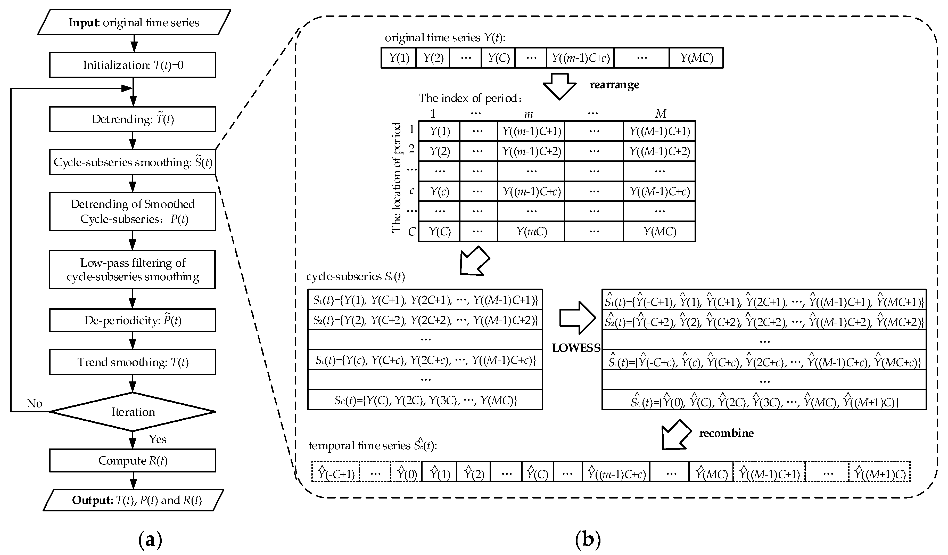
For in-sample decomposition, PTD is an iterative method which is similar to STL. The flow chart of PTD is shown in Figure 2. During each iteration process, periodicity and trend are respectively updated by periodic smoothing and trend smoothing. Suppose Y(t) denotes the original traffic flow, C and M denote the length of one period and the number of periods, respectively. Thus, the number of samples Y(t) is MC. In the initialization, the trend is set as T(t) = 0, t = 1, 2,..., MC. The loop process is composed of six steps, as follows:
  • Step 1: Detrending. Trend T(t) is removed from original data Y(t), then de-trended series T ˜ ( t ) is obtained:
    T ˜ ( t ) = Y ( t ) - T ( t )
  • Step 2: Cycle-subseries smoothing. The details of this step are displayed in Figure 2b. Each cycle-subseries Sc(t) of T ˜ ( t ) is smoothed by LOWESS with K1, and extended one period forward and backwards. Specifically, for independent variables X = [1, 2, 3, 4, …, M]T and dependent variables Y = S c ( t ) = [ Y ( c ) , Y ( C + c ) , Y ( 2 C + c ) , , Y ( ( M 1 ) C + c ) ] T , the estimated values Y ^ c are estimated by LOWESS with K1 at X = [0, 1, 2, 3, 4,…, M, M + 1]T, then all the Y ^ c , c = 1, 2,..., C are arranged in chronological order. Finally, they are recombined and generate temporal time series S ^ ( t ) , t = −C + 1, −C + 2,..., MC + C. The cycle-subseries Sc(t) represents a series composed of elements at the same position of each period, as follows:
    S c ( t ) = { Y ( c ) , Y ( C + c ) , Y ( 2 C + c ) , , Y ( ( M 1 ) C + c ) ) } , c = 1 , 2 , , C
  • Step 3: Low-pass filtering of the cycle-subseries smoothing. The temporal time series S ^ ( t ) , t = −C + 1, −C + 2,..., MC + C are smoothed by a low-pass filter to obtain the series L(t), t = 1, 2,..., MC. The low-pass filter consists of a moving average of length C, followed by another moving average of length C, followed by another moving average of 3, and followed by LOWESS smooth with K2.
  • Step 4: Detrending of Smoothed Cycle-subseries. The preliminary periodicity is calculated as:
    F ( t ) = S ^ ( t ) L ( t ) , t = 1 , 2 , , M C
In the original STL method [49], F(t) is regarded as a seasonal component, which shows obvious periodicity. However, the values at the same time in each period have a few differences. Thus, it is unable to directly forecast future values by cycling. In this study, this component is normalized with the further process as the following: firstly, one period length time series of periodicity Q(t), t = 1, 2,..., C is computed as:
Q ( t ) = 1 M m = 0 M 1 F ( m C + t ) ,   t = 1 , 2 , .. , C
Then, the Q(t) is extended to M periods to obtain the whole periodicity P(t), t = 1, 2,..., MC.
  • Step 5: De-periodicity. The original series Y(t) subtracts the periodicity P(t) to obtain a periodically adjusted series P ˜ ( t ) :
    P ˜ ( t ) = Y ( t ) P ( t )
  • Step 6: Trend smoothing. the P ˜ ( t ) is smoothed by LOWESS with K3 to obtain the trend T(t) = 0, t = 1, 2,..., MC.
After completing iterations, the remainder R(t) = 0, t = 1, 2,..., MC is calculated as:
R ( t ) = Y ( t ) - T ( t ) - P ( t )
Following the above steps, the original times series Y(t) is decomposed into three additive components: trend Y(t), periodicity P(t) and remainder R(t), as Equation (5) expressed.

3.1.3. Decomposition for Out-Of-Sample

Owing to the dynamicity of real-time traffic flow, new data will come as time goes on. Hence, traffic flow data is also updated simultaneously. The new coming data is regarded as out-of-sample. The proposed PTD also provides the method to decompose out-of-sample data in a timely manner, which can satisfy the demand of real-time traffic flow forecasting.
For a new coming data zt at time t, it can also be disaggregated into three additive components, including trend tt, periodicity pt and remainder rt as the following four steps:
  • Step 1: Calculating periodicity. The periodicity pt is calculated according to its position of the period in Q(t) (obtained from Equation (9)).
  • Step 2: De-periodicity. The original data zt subtract the periodicity pt to obtain a periodically adjusted datum z ˜ t :
    z ˜ t = z t p t
  • Step 3: Calculating trend component. The periodically adjusted datum z ˜ t is appended to the end of the periodically adjusted series P ˜ ( t ) (obtained from Equation (10)). The next point of the new series is evaluated by LOWESS with K4, to obtain trend tt.
  • Step 4: Calculating remainder. The remainder rt is computed as:
    r t = z t t t p t
Following the above four steps, the out-of-sample of traffic flow data is decomposed into trend tt, periodicity pt and remainder rt.

3.2. Prediction Models for the Decomposed Components

After completing decomposition, the prediction models are implemented to forecast trend and residual. In order to test the universal applicability of the proposed hybrid method, four well-established prediction models, including both statistical and AI models, are separately combined with PTD. The four prediction models are ARIMA, SVR, ANN, and LSTM. Periodicity is predicted by cycling in the place of modelling since it is a strict period function.

3.2.1. Autoregressive Integrated Moving Average (ARIMA)

ARIMA is a statistical time series model proposed by Bartholomew et al. [55], based on the assumption of stationarity and linearity of time series. Generally, ARIMA is composed of three parts: autoregressive (AR), integration (I) and moving average (MA). The performance of ARIMA is affected by three parameters: autoregressive order p, difference order d and moving average order q. The ARIMA (p,d,q) model can be expressed as follows:
d x ^ t = φ 0 + φ 1 x t 1 + + φ p x t p + ε t θ 1 ε t 1 θ q ε t q
where = ( 1 B ) refers to the backward shift operator for B(x) = xt−1, x ^ t is the predicted value, εt is the residual component distributed as Gaussian distribution with zero mean and σ2 variance.
The difference order d is relevant to the difference method which can convert a nonstationary time series to a stationary time series. In this study, the augmented Dickey–Fuller (ADF) test (unit root test) is utilized, to diagnose the stationarity of traffic flow and determined the parameter d. In addition, the parameters p and q are selected based on the minimum Bayesian information criterion (BIC) value, as follows:
BIC = k ln ( n ) 2 ln ( L )
where k is the number of model parameters; n is the number of samples; L is the maximum likelihood value.

3.2.2. Support Vector Regression (SVR)

Initially, a support vector machine (SVM) was proposed by Boser et al. [56] to solve classification problems, and Cortes and Vapnik [57] extended SVM for regression problems and renamed it as support vector regression (SVR). SVR is based on the structured risk minimization principle, which minimizes the upper bound of the generalization error by using subset data points (i.e., support vectors). For time series modelling, the output of SVR is expressed as:
x ^ t = f ( x t - 1 ) = w T φ ( x t - 1 ) + b
where x ^ t is the predicted value; xt−1 = [xt−1,xt−2,…,xtn]T is input vector with n time lag; w and b are weights and bias, respectively; φ(x) represents the nonlinear mapping function and maps input space x into a high-dimensional feature. In this study, ε-SVR is employed and slack variables ξ and ξ* are introduced. The slack variables measure the errors which occurred by values outside the boundaries, and errors are determined by the ε-tube. The SVR is an optimization problem with objective function as Equation (17) and constraints as Equation (18).
min w , b , ξ , ξ * 1 2 w 2 + H i = 1 m ( ξ i + ξ i * )
subject   to :   { w T φ ( x i ) + b y i ε + ξ i y i w T φ ( x i ) b ε + ξ i * ξ i , ξ i * 0
where H (H > 0) represents the regularization factor; m represents the number of training samples.
If this optimization problem can be transformed into a dual problem, then the SVR function can be expressed as follows:
f ( x ) = i = 1 m ( α i α i ) κ ( x i , x )
where αi and αi* are the Lagrange multipliers; κ(xi,x) is the kernel function that equals the inner product of φ(xi) and φ(x). The radial basis function (RBF) is widely used as kernel function in previous literature [5,12,19,41], and it is also adopted in this study. BRF is expressed as:
κ ( x i , x ) = exp ( γ x i x 2 )
where γ is the coefficient of RBF.

3.2.3. Artificial Neural Network (ANN)

ANN is abstracted from neurons in the human brain. ANN has the universal approximation ability, which indicates that ANN can estimate any nonlinear continuous function up to any desired degree of accuracy. Hence, this model has a good ability to model nonlinear data. Because of this advantage, ANN has been widely introduced and developed for prediction tasks, as well as traffic flow forecasting. A typical ANN model consists of three parts: an input layer, a hidden layer, and an output layer. The structure of ANN is flexible and it depends on the number of neurons in each layer. In this paper, a one-hidden-layer and single-output neural network is employed. The relationship between the output xt and the inputs xt−1, xt−2, …, xtn is expressed as follows:
x t = σ ( b 0 + i = 1 u b i σ ( a i 0 + j = 1 n a i j x t j ) ) + ε t
where aij, j = 1, 2, …, n, represent connection weights from the input layer to hidden neuron ith; ai0 represents the biases in hidden neuron ith; bi, i = 1, 2, …, u, represents connection weights from hidden layer to output neuron; b0 represents the bias in output neuron; n and u are the number of input neurons and hidden neurons, respectively; and εt is the error term. The σ(x) is the sigmoid activation function and is formulated as follows:
σ ( x ) = 1 1 + e x
Therefore, the ANN model in fact performs a nonlinear functional mapping from the historical values xt−1, xt−2, …, xtn to the future value xt:
x t = f ANN ( x t - 1 , x t - 2 , , x t - n ) + ε t

3.2.4. Long Short-Term Memory Neural Network (LSTM)

LSTM is proposed by Hochreiter and Schmidhuber [58] to model for time series data. LSTM is different to traditional ANN in terms of the hidden layers. The hidden neurons of LSTM are designed specially to capture the temporal characteristics. It is realized through one memory cell and 3 gates of input gate, forget gate and output gate. At time t, input gate processes new coming data and the state of the memory cell at time t−1. Forget date decides when to forget the information of memory cell and selects the optimal lag for the input time series. Output gate controls the output information transmitting to the next neural layer. Suppose xt denotes the input time series at t time; it, ft and ot denote the state of input gate, forget gate and output gate, respectively; ct−1 denotes the state of the memory cell at t−1 time. The equations to update the three gates are expressed as follows:
i t = σ ( w i x t + u i c t 1 + b i )
f t = σ ( w f x t + u f c t 1 + b f )
o t = σ ( w o x t + u o c t 1 + b o )
At time t, the state of memory cell ct is controlled by input gate it, forget gate ft and the last time state of memory cell ct−1:
c t = f t c t 1 + i t tanh ( w c x t + u c c t 1 + b c )
The information of LSTM unit output to next layer units is controlled by output gate ot and the state of memory cell ct:
h t = o t tanh ( c t )
where ht represents the final output of hidden neuron; operator “◦” is Hadamard product; wi, wf, wo, wc, ui, uf, uo and uc are connection weights; bi, bf, bo and bc are activation biases; σ(x) and tanh(x) are activation functions; σ(x) is expressed as Equation (22) and tanh(x) is expressed as: tanh(x) = (exex)/(ex + ex).

3.3. Multi-Step Prediction

One-step prediction is extensively studied in the previous study [6,7,12,19,32,38], whereas, it cannot always satisfy the applications in ITS. In this study, a multi-step prediction strategy is well-designed for the proposed hybrid method.
Firstly, predict periodicity. Periodicity is predicted by cycling. Since the periodicity P(t) extracted from PTD is a strictly function with C period length (see Equation (9)), the predicted value at time t is the same to historical value at time tC:
p ^ t = p t - C ; p ^ t + 1 = p t - C + 1 ;
Secondly, predict trend and remainder respectively. The iterated strategy, which is widely used in multi-step time series forecasting, is adopted to the multi-step prediction of trend and remainder. Based on an already constructed model with one-step prediction, the iterated strategy uses the predicted value as an input for the same model to forecast the next time value (see Equation (30)). This process is iterated up to the maximum prediction horizon. The iterated strategy has two outstanding advantages: one is that only one model must be established. The other is that the prediction steps are unlimited.
t ^ t = f T ( t t - 1 , t t 2 , , t t n ) ; r ^ t = f R ( r t - 1 , r t 2 , , r t n ) t ^ t + 1 = f T ( t ^ t , t t - 1 , , t t n + 1 ) ; r ^ t + 1 = f R ( r ^ t , r t - 1 , , r t n + 1 ) ;
where tt and rt respectively represent the true values of trend and remainder at time t; t ^ t and r ^ t respectively represent the predicted values of trend and remainder at time t; fT and fR represent the already constructed model for trend and remainder, respectively.
Lastly, the predicted values of the three components are summed as final outcomes y ^ t :
y ^ t = t ^ t + p ^ t + r ^ t y ^ t + 1 = t ^ t + 1 + p ^ t + 1 + r ^ t + 1

3.4. Hybrid Prediction Models

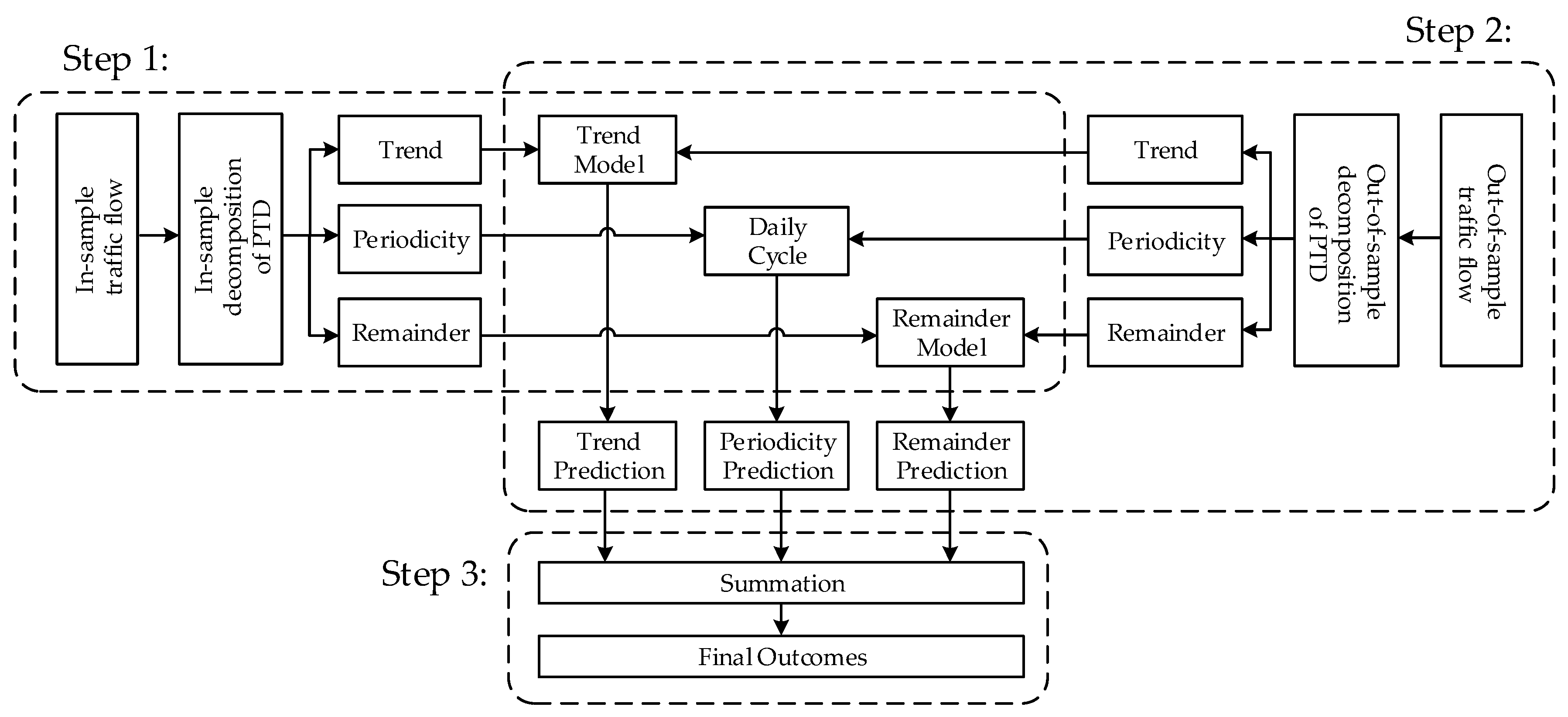
Based on the principle of “decomposition first and forecasting last”, the procedure of the proposed hybrid method for traffic flow forecasting is displayed in Figure 3; it contains three steps, as listed:
  • Step 1: In-sample decomposition and models training. Based on the in-sample decomposition of PTD, the in-sample data is decomposed into three components: trend, periodicity, and remainder. Then, each component is used to train the models (described in Section 3.2) separately.
  • Step 2: Out-of-sample decomposition and multi-step prediction. Based on the out-of-sample decomposition of PTD, the out-of-sample data is also decomposed into trend, periodicity, and remainder. Then, each component of out-of-sample decomposition is input into the corresponding trained model. The predicted results are obtained from the output of the models.
  • Step 3: Integration for the final outcomes. The predicted results of the three components are summed as the final outcomes.

4. Experiments

4.1. Data Description

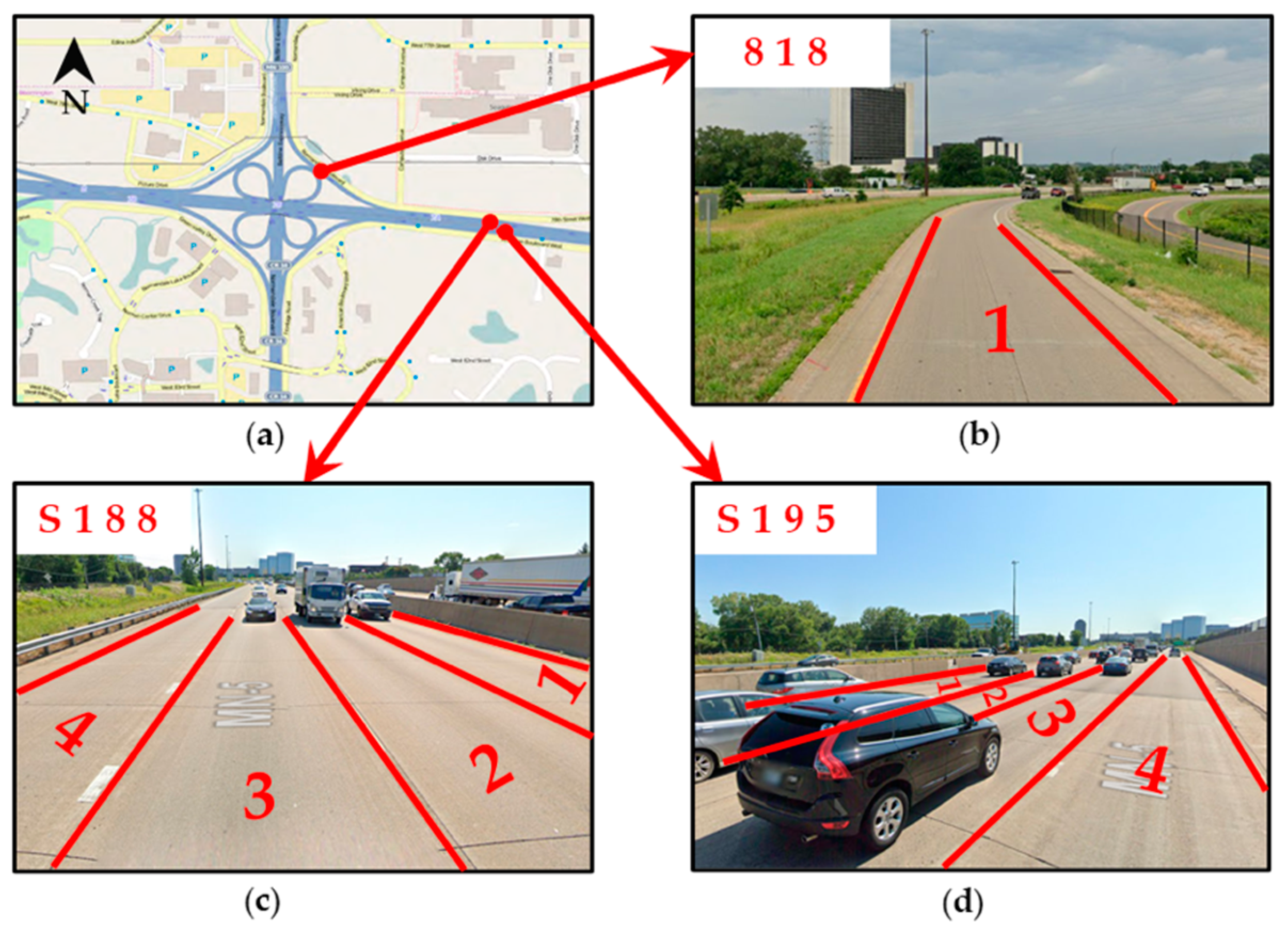
In this study, the traffic flow data are available from the Minnesota Department of Transportation (Mn/DOT) [59]. The Mn/DOT provides traffic volume and occupancy data with a 30-second interval of freeways in Minnesota, USA. In our experiments, only traffic volume data are used, and the data are collected from three detection stations (i.e., S188, S195 and 818) at the interchange of I-494 and TH100 (see Figure 4). As shown in Figure 4, S188 and S195 are located in two opposite directions of I-94 freeway and 818 is located at an exit ramp. The three cases with different patterns are used to test the adaptability of the hybrid models. We selected four weeks of data, from 29 April to 24 May in 2019. Since the patterns of traffic volume on weekdays and weekends are different, the data on weekends is discarded. The original traffic volume data is aggregated into a 5-minute interval referred to in previous studies [4,5,14,21,60]. The data of the first two weeks are used as the training dataset (i.e., from 29 April to 10 May, 2880 samples totally) to train the models. The next week is used as the validation dataset (i.e., from 12 to 16 in May, 1440 samples totally) to determine the hyper-parameters of the models. The last week (i.e., from 20 to 24 in May, 1440 samples totally) is used as the testing dataset to evaluate the prediction results.
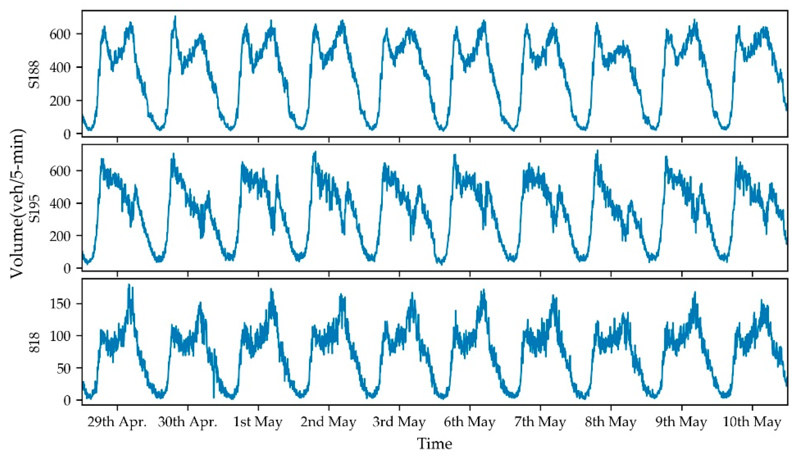
The training dataset of collected traffic volume is shown in Figure 5. It can be seen that the three stations have different distributions, which is to evaluate the adaptability of proposed hybrid models. The distribution features of traffic flow are agreed to their locations: S188 and S195 are located at the four-lane highway with large traffic volume in the daytime, and the peak-volume of these two stations are both over 600 vehicles per 5-minute; 818 is located at the ramp with only one lane and the traffic volume is much smaller, and the peak volume of it is about 180 vehicles per 5-minute. Furthermore, S188 has two obvious peaks in the morning and afternoon, and S195 only has one peak in the morning. Moreover, 818 only has one peak in the afternoon. Despite different distributions and peak patterns, all the three stations have obvious one-day periodicity.

4.2. Design of Experiments

To demonstrate the contribution of the proposed PTD approach, four hybrid models combining PTD (i.e., PTD-ARIMA, PTD-SVR, PTD-ANN and PTD-LSTM) and four individual models (i.e., ARIMA, SVR, ANN and LSTM) are employed to experiment and comparatively analyze by using the prepared data.
In the PTD procedure, the training datasets are regarded as in-sample, and the validation datasets and testing datasets are regarded as out-of-sample, to simulate real-time traffic flow. The period length C is 288 (i.e., 24 (hour) * 60 (minute)/5 (minute) = 288), and the period number M is 10 (i.e., workdays of two weeks). According to the studies [49,53,54], the nearest neighbor number K of LOWESS should be set to cover one-period length. In our study, for in-sample decomposition, the LOWESS smoothen original series contains both past and future. Consequently, K1, K2, and K3 (see Step 2, Step 3, and Step 6 in Section 3.1.2.) are all set as 144. Meanwhile, for out-of-sample decomposition, the LOWESS smoothen original times series containing only past and K4 (see Step 4 in Section 3.1.3.) is set as 288.
In the prediction stage, the Min-Max normalization technology (expressed as Equation (32)) is employed to scale the data into the range of [0, 1] before feeding into the model. This technology can accelerate learning and convergence during training model. The outputs of the model are rescaled by reversed Min-Max normalization (expressed as Equation (33)), to obtain the final predicted results.
x = x min ( x ) max ( x ) min ( x )
x = x × ( max ( x ) min ( x ) ) + min ( x )
It is worth noting that the hyper-parameters of prediction models can significantly affect their performance. Hence, the well-established grid-search and cross-validation method is implemented, to select appropriate hyper-parameters for each model. Specifically, all the models with different hyper-parameters are trained by the same training dataset, but only the model which has the best performance on validation dataset is selected. The models with determined hyper-parameters are evaluated by testing dataset. The critical hyper-parameters in each model are as follows:
  • ARIMA: the difference order d of ARIMA is set based on ADF unit root test and the autoregressive order p and moving average order q are both selected from 0 to 24, based on minimum BIC value (see Equation (15)).
  • SVR: The RBF kernel function coefficient γ, and the regularization factor H, the tube width ε are all selected from {10−5, 10−4, 10−3, 10−2, 10−1, 1, 10, 102, 103, 104}.
  • ANN: According to previous research [30,31], a one-hidden-layer neural network is frequently utilized and also adopted in our experiment. The number of hidden neurons u is selected from 2 to 40 with step 2. The model is optimized by Adam algorithm with mean square error (MSE) loss function. The learning rate is set as 0.001, the batch-size is 256, and the epochs is 500.
  • LSTM: A one-hidden-layer LSTM is utilized reference to existing studies [9,34,60]. The number of hidden neurons is also selected from 2 to 40 with step 2, and the other hyper-parameters are the same as ANN.
In addition, the input step is set as 12 and output step is set as 1. The prediction horizons are set as 6. The final determined hyper-parameters are shown in Table 2. The periodicity is not in this table, because this component can be predicted by cycling.

4.3. Performance Measures

In our study, three widely used measures are utilized to evaluate the performance of models, including mean absolute error (MAE), mean absolute percentage error (MAPE) and mean square error (MSE). Denote true value and predicted value as yt and y ^ i , respectively; n is the number of testing data. The equations are expressed as follows:
MAE = 1 n i = 1 n | y i y ^ i |
MAPE = 1 n i = 1 n | y i y ^ i y i | × 100 %
MSE = 1 n i = 1 n ( y i y ^ i ) 2

5. Results and Discussions

5.1. Analysis of Decomposition Results

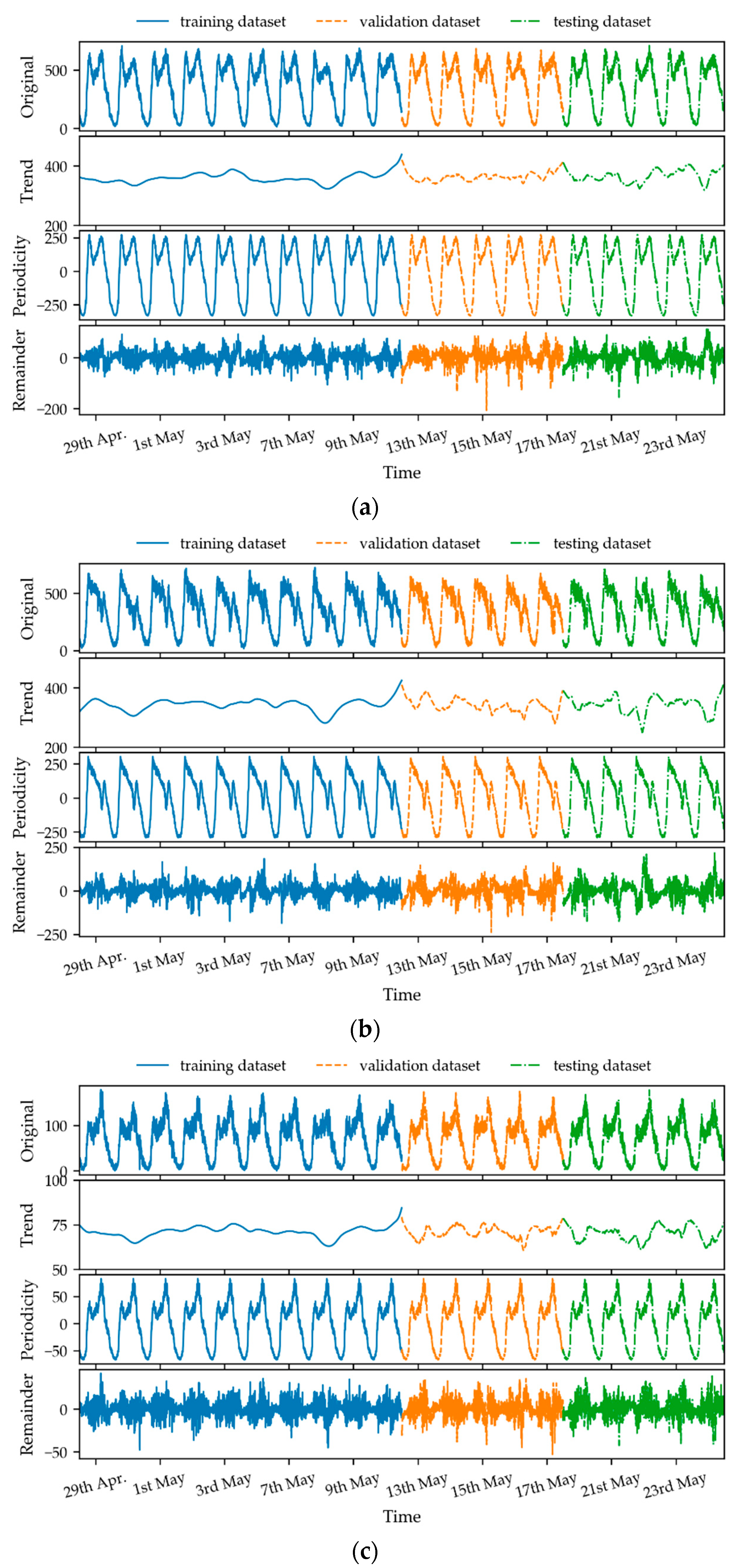
The decomposition results are shown in Figure 6. It can be seen that the original traffic flow is decomposed into trend, periodic, and remainder components. For trend, this component shows the day-to-day characteristics, and it fluctuates moderately. Furthermore, trend extracted through in-sample decomposition (i.e., training dataset) is smoother than that through out-of-sample decomposition (i.e., validation dataset and testing dataset). The reason for this is that the trend is extracted by bilateral smoothness, containing both past and future during in-sample decomposition. Meanwhile, during out-of-sample decomposition, the trend is extracted through only past smoothness. The periodicity shows the within-day characteristics and it is a strict period function, which means the values at the same time on different days are identical. The peak features of traffic flow are also distinctly displayed in periodicity, which is consistent with the original data. As for the remainder, it fluctuates irregularly and can be regarded as noise.

5.2. Analysis of Prediction Results

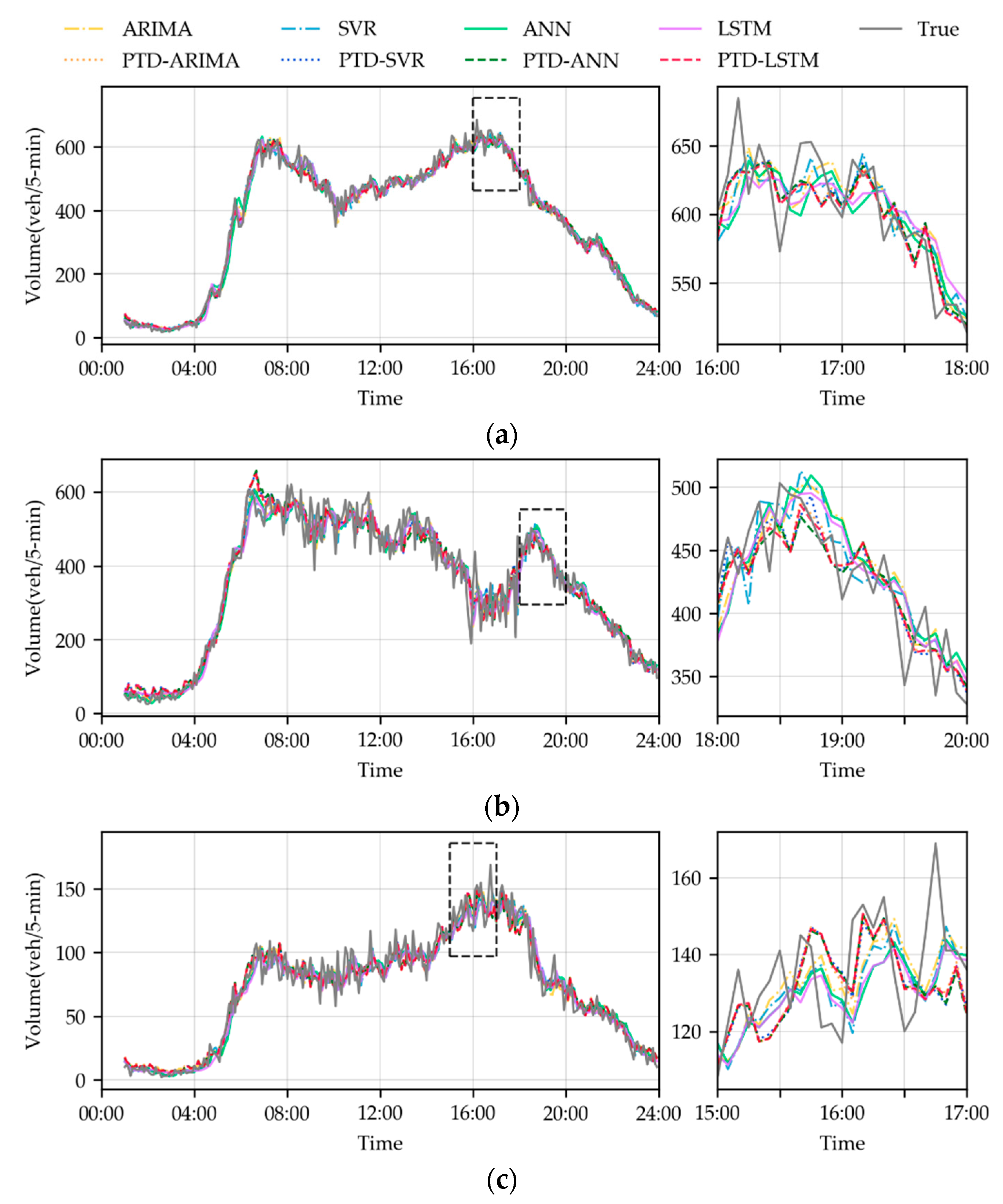
Each component is predicted separately, and the final outcomes are obtained by summing the three predicted results. Taking the first day of the testing dataset (i.e., 20 May 2019) as an example, the true values and one-step predicted results are shown in Figure 7. The left subplots are the whole day predicted results, and the right subplots zoom in on two rush hours in the evening. It is apparent that the predicted results of hybrid models are closer to true values than those results of individual models, which indicates that the hybrid models perform better. In addition, the predicted results of the four hybrid models are almost the same, which suggests that the four models combining PTD have almost similar performances.
Table 3 provides the average measures evaluated across all the six-step prediction horizons. Overall, all hybrid models perform better than individual models. Among hybrid models, it seems that there is no specific hybrid model that always performs best in all testing cases. However, after further investigation, it is found that the gaps among different hybrid models are slightly small. In particular, the differences of MAE among different hybrid models are less than 1. This finding suggests that combination with PTD is a universally applicable method to improve prediction accuracy effectively. In addition, the improved items represent the improved performance from the hybrid model to the individual model. This item can also be regarded as the contribution of PTD approach to reduce the prediction errors. On average, the MAE, MAPE and MSE are respectively reduced by 23%, 25% and 39% on station S188, 11%, 11% and 19% on station S195, and 16%, 13% and 28% on station 818. Over all testing stations, the hybrid method reduces the MAE, MAPE, and MSE by 17%, 17%, and 29%. These results demonstrate that the hybrid models combining PTD are superior to the individual models.
There is one thing that we need to explain; it seems that the testing models do not perform so well in case 818, in terms of MAPE. The MAPE of the best model PTD-LSTM is close to 20%. This is because that MAPE is sensitive to small true values (i.e., the yi in Equation (35)). The traffic volume of 818 is much smaller than S188 and S195 (see Figure 5). When the value in the denominator is small, a small deviation in error will create a large change in the absolute percentage error (APE). For example, suppose two samples y1 = 10 and y2 = 100, and the predicted values of them are y ^ 1 = 20 and y ^ 2 = 110 . The absolute error (AE) and square error (SE) of them are equal (i.e., AE1 = AE2 = 10 and SE1 = SE2 = 102 = 100). However, the APE of them is quite different (i.e., APE1 = 100% and APE2 = 10%). When the AEs or SEs are equal, the true values are smaller; the APEs are larger. As for MSEs and MAEs, these results are normal because the models are trained based on MSE loss.

5.3. Analysis of Multi-Step Prediction Errors

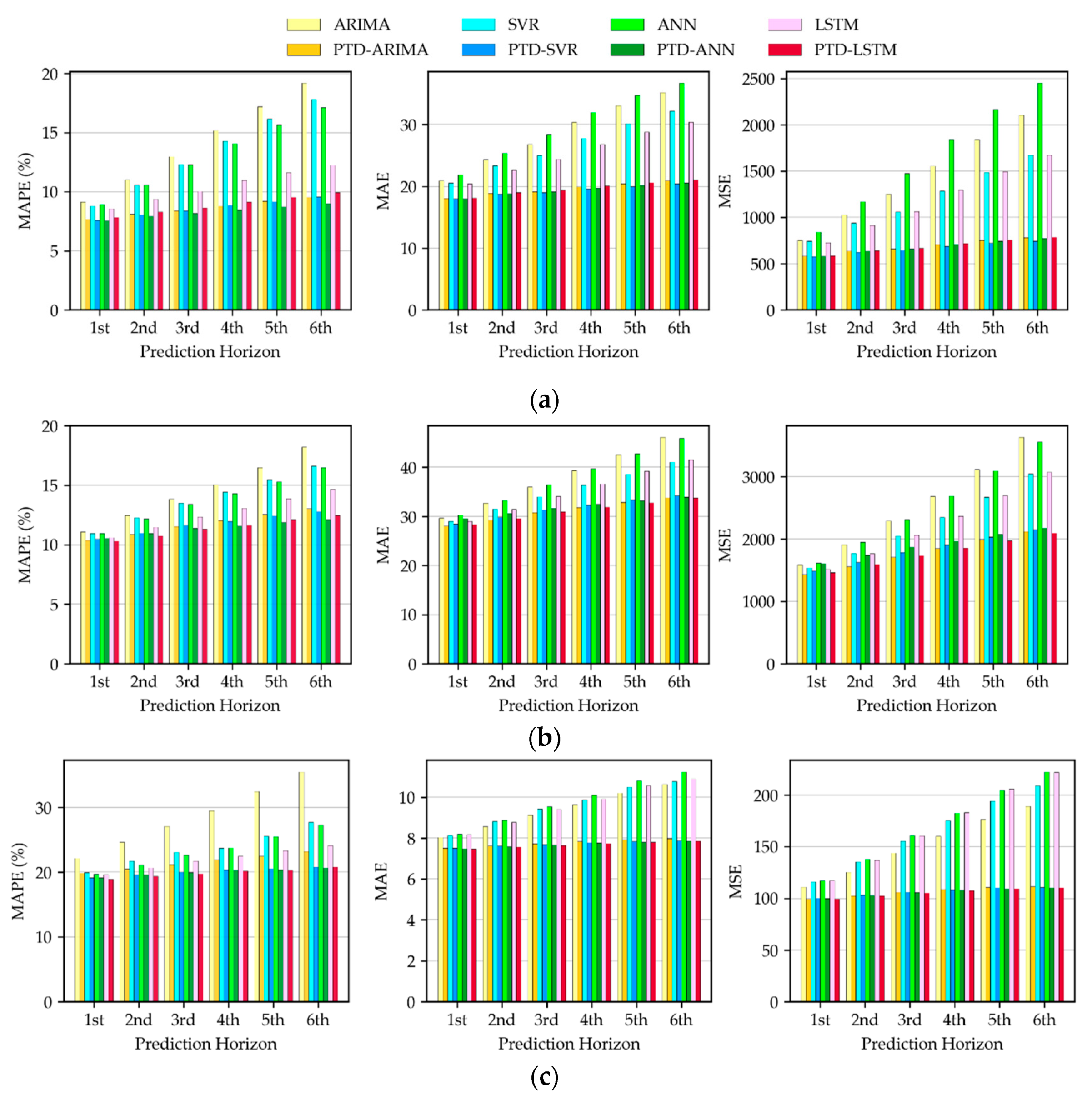
In order to analyze the multi-step prediction errors, the evaluation measures of each prediction horizon are presented in Figure 8. An aspect that should be noted is that all prediction errors increase along prediction horizons. This is owing to the cumulative errors, which stem from feeding predicted values into the models during a multi-step prediction. What stands out in this figure is that the errors of the individual models increase more rapidly along with prediction horizons than the hybrid models. Furthermore, the increased rates of hybrid models are almost the same. These findings indicate that no matter which prediction model it is integrated into, the hybrid model can always reduce cumulative errors effectively.
To elaborate on the contribution of PTD, the rate of reduced error is introduced, which is equal to the reduced error divided by the error of the individual model. The rates are computed and plotted in Figure 9. The negative rate represents that the hybrid model performs better than the corresponding individual model. The absolute value of the rate is larger, the improvement of performance is larger. It is apparent that the rates of reduced errors decline, along with prediction horizons. This represents that hybrid models are able to reduce the cumulative errors. The PTD approach can decompose the complex traffic flow into trend, periodicity, and remainder. These components vary more regularly and are modelled more easily. This is why the hybrid method can improve the prediction performance. From these findings, it demonstrates that the method combining PTD shows robustness for multi-step traffic flow forecasting.

6. Conclusions

In this paper, to extract trend and periodic characteristics of traffic flow and achieve more accurate forecasting, a novel method combining PTD is proposed. PTD is developed to decompose the original traffic flow into trend, periodicity, and remainder. Then, the periodicity is predicted by cycling, while the trend and remainder by modelling. To test the applicability of the proposed method for different traffic flow patterns, three datasets with different distributions collected from Mn/DOT are utilized to conduct experiments and analyze comparatively. Our main work is concluded as follows:
  • A novel decomposition approach for traffic flow PTD is formulated. Fully considering the dynamicity of real-time traffic flow, PTD is formulated to decompose both in-sample and out-of-sample data. This approach can decompose the original traffic flow into trend, periodicity, and remainder.
  • A novel hybrid method combining PTD for traffic flow forecasting is developed. To demonstrate the universal applicability of the PTD approach, both statistical and AI models (i.e., ARIMA, SVR, ANN, LSTM) are combined with PTD, to establish hybrid models (i.e., PTD-ARIMA, PTD-SVR, PTD-ANN and PTD-LSTM). Empirical results show that the MAE, MAPE, and MSE of hybrid models are averagely reduced by 17%, 17%, and 29% than individual models, respectively.
  • After investigating multi-step prediction results, it is found that the hybrid models combining PTD can not only reduce the prediction errors, but also reduce cumulative errors. It suggests that the proposed hybrid method is robust for multi-step traffic flow forecasting.
Three limitations remain in our study and will be addressed in future study. Firstly, only traffic flow data on workdays is studied. The patterns of traffic flow in weekdays are different to that on weekends. In future studies, the PTD approach will be improved for whole week traffic flow decomposition. Secondly, only traffic volume data are tested and evaluated. In further studies, other measures of traffic status (such as traffic speed, travel time) will be collected to carry out experiments. Thirdly, only historical data are considered. In further studies, the spatial-temporal features or topology features of the road network will be considered for a more accurate prediction.

Author Contributions

Conceptualization, W.Z., W.W. and X.H.; Data curation, W.Z. and X.H.; Formal analysis, W.Z.; Funding acquisition, W.W. and X.H.; Investigation, W.Z. and Y.Z.; Methodology, W.Z.; Project administration, W.W. and X.H.; Resources, W.Z. and W.W.; Software, W.Z.; Supervision, W.W. and X.H.; Validation, W.Z.; Visualization, W.Z.; Writing—original draft, W.Z.; Writing—review and editing, W.Z., W.W., X.H. and Y.Z. All authors have read and agreed to the published version of the manuscript.

Funding

This research was funded by the National Natural Science Foundation of China, grant number 51878166 and 71801042; Natural Science of Jiangsu Province, grant number BK20180381.

Acknowledgments

The authors are grateful to the Minnesota Department of Transportation (Mn/DOT) for opening the traffic flow data.

Conflicts of Interest

The authors declare no conflict of interest. The funders had no role in the design of the study; in the collection, analyses, or interpretation of data; in the writing of the manuscript, or in the decision to publish the results.

References

  1. Zahid, M.; Chen, Y.; Jamal, A.; Mamadou, C.Z. Freeway short-term travel speed prediction based on data collection time-horizons: A fast forest quantile regression approach. Sustainability 2020, 12, 646. [Google Scholar] [CrossRef] [Green Version]
  2. Vlahogianni, E.I.; Karlaftis, M.G.; Golias, J.C. Short-term traffic forecasting: Where we are and where we’re going. Transp. Res. Part C Emerg. Technol. 2014, 43, 3–19. [Google Scholar] [CrossRef]
  3. Chen, X.; Lu, J.; Zhao, J.; Qu, Z.; Yang, Y.; Xian, J. Traffic flow prediction at varied time scales via ensemble empirical mode decomposition and artificial neural network. Sustainability 2020, 12, 3678. [Google Scholar] [CrossRef]
  4. Lv, Y.; Duan, Y.; Kang, W.; Li, Z.; Wang, F.Y. Traffic Flow Prediction with Big Data: A Deep Learning Approach. IEEE Trans. Intell. Transp. Syst. 2015, 16, 865–873. [Google Scholar] [CrossRef]
  5. Zhang, M.; Zhen, Y.; Hui, G.; Chen, G. Accurate multisteps traffic flow prediction based on SVM. Math. Probl. Eng. 2013, 2013. [Google Scholar] [CrossRef] [Green Version]
  6. Luo, X.; Li, D.; Yang, Y.; Zhang, S. Spatiotemporal traffic flow prediction with KNN and LSTM. J. Adv. Transp. 2019, 2019. [Google Scholar] [CrossRef] [Green Version]
  7. Jiang, X.; Adeli, H. Dynamic wavelet neural network model for traffic flow forecasting. J. Transp. Eng. 2005, 131, 771–779. [Google Scholar] [CrossRef]
  8. Bratsas, C.; Koupidis, K.; Salanova, J.M.; Giannakopoulos, K.; Kaloudis, A.; Aifadopoulou, G. A comparison of machine learning methods for the prediction of traffic speed in Urban places. Sustainability 2020, 12, 142. [Google Scholar] [CrossRef] [Green Version]
  9. Ma, X.; Tao, Z.; Wang, Y.; Yu, H.; Wang, Y. Long short-term memory neural network for traffic speed prediction using remote microwave sensor data. Transp. Res. Part C 2015, 54, 187–197. [Google Scholar] [CrossRef]
  10. Wang, H.; Liu, L.; Dong, S.; Qian, Z.; Wei, H. A novel work zone short-term vehicle-type specific traffic speed prediction model through the hybrid EMD–ARIMA framework. Transp. B 2016, 4, 159–186. [Google Scholar] [CrossRef]
  11. Yang, J.S. Travel time prediction using the GPS test vehicle and Kalman filtering techniques. In Proceedings of the American Control Conference, Portland, OR, USA, 8–10 June 2005; Volume 3, pp. 2128–2133. [Google Scholar] [CrossRef]
  12. Zhang, Y.; Liu, Y. Traffic forecasting using least squares support vector machines. Transportmetrica 2009, 5, 193–213. [Google Scholar] [CrossRef]
  13. Zou, Y.; Hua, X.; Zhang, Y.; Wang, Y. Hybrid short-term freeway speed prediction methods based on periodic analysis. Can. J. Civ. Eng. 2015, 42, 570–582. [Google Scholar] [CrossRef]
  14. Min, W.; Wynter, L. Real-time road traffic prediction with spatio-temporal correlations. Transp. Res. Part C Emerg. Technol. 2011, 19, 606–616. [Google Scholar] [CrossRef]
  15. Ahmed, M.S.; Cook, A.R. Analysis of Freeway Traffic Time-Series Data By Using Box-Jenkins Techniques. Transp. Res. Rec. 1979, 1–9. [Google Scholar]
  16. Li, L.; Qin, L.; Qu, X.; Zhang, J.; Wang, Y.; Ran, B. Day-ahead traffic flow forecasting based on a deep belief network optimized by the multi-objective particle swarm algorithm. Knowl.-Based Syst. 2019, 172, 1–14. [Google Scholar] [CrossRef]
  17. Tselentis, D.I.; Vlahogianni, E.I.; Karlaftis, M.G. Improving short-term traffic forecasts: To combine models or not to combine? IET Intell. Transp. Syst. 2015, 9, 193–201. [Google Scholar] [CrossRef]
  18. Lin, L.; Wang, Q.; Huang, S.; Sadek, A.W. On-line prediction of border crossing traffic using an enhanced Spinning Network method. Transp. Res. Part C Emerg. Technol. 2014, 43, 158–173. [Google Scholar] [CrossRef]
  19. Luo, X.; Li, D.; Zhang, S. Traffic flow prediction during the holidays based on DFT and SVR. J. Sens. 2019, 2019. [Google Scholar] [CrossRef] [Green Version]
  20. Kolidakis, S.; Botzoris, G.; Profillidis, V.; Lemonakis, P. Road traffic forecasting—A hybrid approach combining Artificial Neural Network with Singular Spectrum Analysis. Econ. Anal. Policy 2019, 64, 159–171. [Google Scholar] [CrossRef]
  21. Guo, F.; Krishnan, R.; Polak, J.W. Short-term traffic prediction under normal and incident conditions using singular spectrum analysis and the k-nearest neighbour method. In Proceedings of the IET and ITS Conference on Road Transport Information and Control (RTIC 2012), London, UK, 25–26 September 2012. [Google Scholar] [CrossRef]
  22. Chen, W.; Shang, Z.; Chen, Y.; Chaeikar, S.S. A Novel Hybrid Network Traffic Prediction Approach Based on Support Vector Machines. J. Comput Netw. Commun. 2019, 2019. [Google Scholar] [CrossRef]
  23. Shang, Q.; Lin, C.; Yang, Z.; Bing, Q.; Zhou, X. A hybrid short-term traffic flow prediction model based on singular spectrum analysis and kernel extreme learning machine. PLoS ONE 2016, 11. [Google Scholar] [CrossRef] [PubMed]
  24. Zheng, C.; Li, L. The improvement of the forecasting model of short-term traffic flow based on wavelet and ARMA. In Proceedings of the SCMIS 2010—2010 8th International Conference on Supply Chain Management and Information Systems: Logistics Systems and Engineering, Hong Kong, China, 6–9 October 2010. [Google Scholar]
  25. Zhang, N.; Guan, X.; Cao, J.; Wang, X.; Wu, H. Wavelet-HST: A Wavelet-Based Higher-Order Spatio-Temporal Framework for Urban Traffic Speed Prediction. IEEE Access 2019, 7, 118446–118458. [Google Scholar] [CrossRef]
  26. Okutani, I.; Stephanedes, Y.J. Dynamic prediction of traffic volume through Kalman filtering theory. Transp. Res. Part B 1984, 18, 1–11. [Google Scholar] [CrossRef]
  27. Gong, X.; Wang, F. Three improvements on KNN-NPR for traffic flow forecasting. In Proceedings of the IEEE Conference on Intelligent Transportation Systems, Singapore, 6 September 2002; pp. 736–740. [Google Scholar] [CrossRef]
  28. Yu, B.; Song, X.; Guan, F.; Yang, Z.; Yao, B. K-Nearest Neighbor Model for Multiple-Time-Step Prediction of Short-Term Traffic Condition. J. Transp. Eng. 2016, 142. [Google Scholar] [CrossRef]
  29. Xiao, J.; Wei, C.; Liu, Y. Speed estimation of traffic flow using multiple kernel support vector regression. Phys. A Stat. Mech. Appl. 2018, 509, 989–997. [Google Scholar] [CrossRef]
  30. Vlahogianni, E.I.; Karlaftis, M.G.; Golias, J.C. Optimized and meta-optimized neural networks for short-term traffic flow prediction: A genetic approach. Transp. Res. Part. C Emerg. Technol. 2005, 13, 211–234. [Google Scholar] [CrossRef]
  31. Kumar, K.; Parida, M.; Katiyar, V.K. Short term traffic flow prediction in heterogeneous condition using artificial neural network. Transport 2015, 30, 397–405. [Google Scholar] [CrossRef]
  32. Ma, X.; Dai, Z.; He, Z.; Ma, J.; Wang, Y.; Wang, Y. Learning traffic as images: A deep convolutional neural network for large-scale transportation network speed prediction. Sensors 2017, 17, 818. [Google Scholar] [CrossRef] [Green Version]
  33. Smith, B.L.; Demetsky, M.J. Traffic flow forecasting: Comparison of modeling approaches. J. Transp. Eng. 1997, 123, 261–266. [Google Scholar] [CrossRef]
  34. Jia, Y.; Wu, J.; Xu, M. Traffic flow prediction with rainfall impact using a deep learning method. J. Adv. Transp. 2017, 2017. [Google Scholar] [CrossRef]
  35. Zeng, D.; Xu, J.; Gu, J.; Liu, L.; Xu, G. Short term traffic flow prediction using hybrid ARIMA and ANN models. In Proceedings of the 2008 Workshop on Power Electronics and Intelligent Transportation System, PEITS 2008, Guangzhou, China, 2–3 August 2008; pp. 621–625. [Google Scholar] [CrossRef]
  36. Tan, M.C.; Wong, S.C.; Xu, J.M.; Guan, Z.R.; Zhang, P. An aggregation approach to short-term traffic flow prediction. IEEE Trans. Intell. Transp. Syst. 2009, 10, 60–69. [Google Scholar] [CrossRef]
  37. Hou, Q.; Leng, J.; Ma, G.; Liu, W.; Cheng, Y. An adaptive hybrid model for short-term urban traffic flow prediction. Phys. A Stat. Mech. Appl. 2019, 527. [Google Scholar] [CrossRef]
  38. Li, L.; He, S.; Zhang, J.; Ran, B. Short-term highway traffic flow prediction based on a hybrid strategy considering temporal–spatial information. J. Adv. Transp. 2016, 50, 2029–2040. [Google Scholar] [CrossRef]
  39. Chan, K.Y.; Dillon, T.S.; Singh, J.; Chang, E. Traffic flow forecasting neural networks based on exponential smoothing method. In Proceedings of the 2011 6th IEEE Conference on Industrial Electronics and Applications, ICIEA 2011, Beijing, China, 21–23 June 2011; pp. 376–381. [Google Scholar] [CrossRef]
  40. Yang, H.F.; Dillon, T.S.; Chang, E.; Chen, Y.P.P. Optimized Configuration of Exponential Smoothing and Extreme Learning Machine for Traffic Flow Forecasting. IEEE Trans. Ind. Inform. 2019, 15, 23–34. [Google Scholar] [CrossRef]
  41. Hong, W.C.; Dong, Y.; Zheng, F.; Wei, S.Y. Hybrid evolutionary algorithms in a SVR traffic flow forecasting model. Appl. Math. Comput. 2011, 217, 6733–6747. [Google Scholar] [CrossRef]
  42. Zhang, Y.; Huang, G. Traffic flow prediction model based on deep belief network and genetic algorithm. IET Intell. Transp. Syst. 2018, 12, 533–541. [Google Scholar] [CrossRef]
  43. Feng, X.; Ling, X.; Zheng, H.; Chen, Z.; Xu, Y. Adaptive multi-kernel SVM with spatial-temporal correlation for short-term traffic flow prediction. IEEE Trans. Intell. Transp. Syst. 2019, 20, 2001–2013. [Google Scholar] [CrossRef]
  44. Nihan, N.L.; Holmesland, K.O. Use of the box and Jenkins time series technique in traffic forecasting. Transportation 1980, 9, 125–143. [Google Scholar] [CrossRef]
  45. Yang, B.; Sun, S.; Li, J.; Lin, X.; Tian, Y. Traffic flow prediction using LSTM with feature enhancement. Neurocomputing 2019, 332, 320–327. [Google Scholar] [CrossRef]
  46. Li, Z.; Li, Y.; Li, L. A comparison of detrending models and multi-regime models for traffic flow prediction. IEEE Intell. Transp. Syst. Mag. 2014, 6, 34–44. [Google Scholar] [CrossRef]
  47. Chen, C.; Wang, Y.; Li, L.; Hu, J.; Zhang, Z. The retrieval of intra-day trend and its influence on traffic prediction. Transp. Res. Part C Emerg. Technol. 2012, 22, 103–118. [Google Scholar] [CrossRef]
  48. Dai, X.; Fu, R.; Zhao, E.; Zhang, Z.; Lin, Y.; Wang, F.Y.; Li, L. DeepTrend 2.0: A light-weighted multi-scale traffic prediction model using detrending. Transp. Res. Part C Emerg. Technol. 2019, 103, 142–157. [Google Scholar] [CrossRef]
  49. Cleveland, R.B.; Cleveland, W.S.; McRae, J.E.; Terpenning, I. STL: A seasonal-trend decomposition procedure based on loess. J. Off. Stat. 1990, 6, 3–73. [Google Scholar]
  50. Rojo, J.; Rivero, R.; Romero-Morte, J.; Fernández-González, F.; Pérez-Badia, R. Modeling pollen time series using seasonal-trend decomposition procedure based on LOESS smoothing. Int. J. Biometeorol. 2017, 61, 335–348. [Google Scholar] [CrossRef] [PubMed]
  51. Theodosiou, M. Forecasting monthly and quarterly time series using STL decomposition. Int. J. Forecast. 2011, 27, 1178–1195. [Google Scholar] [CrossRef]
  52. Stow, C.A.; Cha, Y.; Johnson, L.T.; Confesor, R.; Richards, R.P. Long-term and seasonal trend decomposition of maumee river nutrient inputs to western lake erie. Environ. Sci. Technol. 2015, 49, 3392–3400. [Google Scholar] [CrossRef]
  53. Xiong, T.; Li, C.; Bao, Y. Seasonal forecasting of agricultural commodity price using a hybrid STL and ELM method: Evidence from the vegetable market in China. Neurocomputing 2018, 275, 2831–2844. [Google Scholar] [CrossRef]
  54. Qin, L.; Li, W.; Li, S. Effective passenger flow forecasting using STL and ESN based on two improvement strategies. Neurocomputing 2019, 356, 244–256. [Google Scholar] [CrossRef]
  55. Bartholomew, D.J.; Box, G.E.P.; Jenkins, G.M. Time Series Analysis Forecasting and Control. Oper. Res. Q. (1970-1977) 1971, 22, 199. [Google Scholar] [CrossRef]
  56. Boser, B.E.; Guyon, I.M.; Vapnik, V.N. Training algorithm for optimal margin classifiers. In Proceedings of the Fifth Annual ACM Workshop on Computational Learning Theory, Pittsburgh, PA, USA, 27–29 July 1992; pp. 144–152. [Google Scholar] [CrossRef]
  57. Cortes, C.; Vapnik, V. Support-vector networks. Mach. Learn. 1995, 20, 273–297. [Google Scholar] [CrossRef]
  58. Hochreiter, S.; Schmidhuber, J. Long Short-Term Memory. Neural Comput. 1997, 9, 1735–1780. [Google Scholar] [CrossRef] [PubMed]
  59. The Minnesota Department of Transportation. Mn/DOT Traffic Data. Available online: http://data.dot.state.mn.us/datatools/ (accessed on 11 March 2020).
  60. Tian, Y.; Pan, L. Predicting short-term traffic flow by long short-term memory recurrent neural network. In Proceedings of the 2015 IEEE International Conference on Smart City, Chengdu, China, 19–21 December 2015; pp. 153–158. [Google Scholar] [CrossRef]
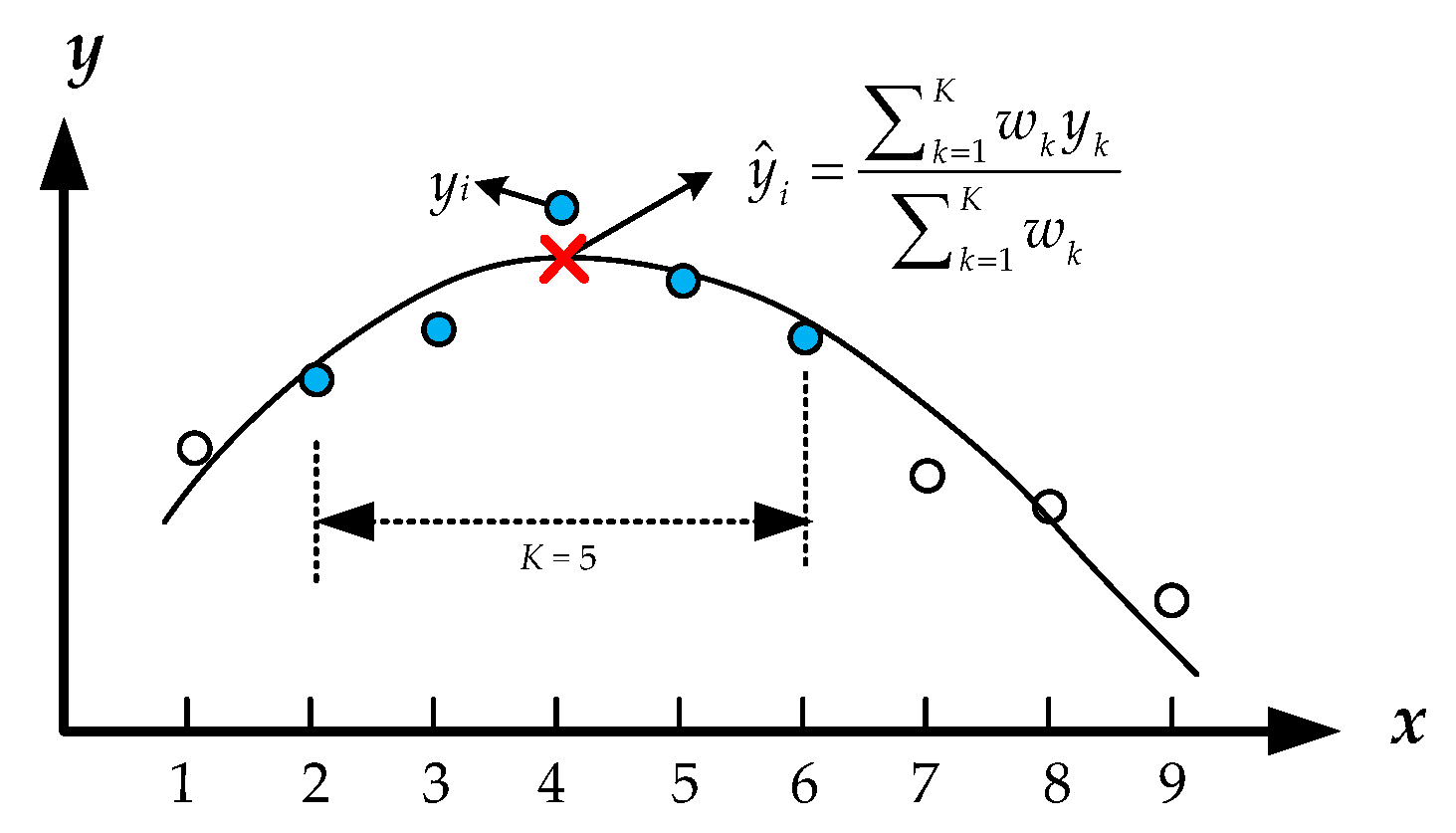
Figure 1. A simple case of LOWESS.
Sustainability 12 05891 g001
Figure 2. The flow chart of PTD for in-sample decomposition: (a) PTD; (b) Cycle-subseries smoothing.
Sustainability 12 05891 g002
Figure 3. The procedure of the proposed hybrid prediction method.
Sustainability 12 05891 g003
Figure 4. The location of selected stations: (a) Interchange of I-494 and TH100; (b) 818; (c) S188; (d) S195.
Sustainability 12 05891 g004
Figure 5. The traffic volume of the training dataset, i.e., from 29 April to 10 May 2019.
Sustainability 12 05891 g005
Figure 6. Decomposition Results: (a) S188; (b) S195; (c) 818.
Sustainability 12 05891 g006
Figure 7. The prediction results of traffic volume. The left subplots are the whole day on 20 May 2019, and the right subplots are two rush hours in the evening: (a) S188; (b) S195; (c) 818.
Sustainability 12 05891 g007
Figure 8. Results of multi-step prediction: (a) S188; (b) S195; (c) 188.
Sustainability 12 05891 g008
Figure 9. Rates of reduced errors: (a) S188; (b) S195; (c) 818.
Sustainability 12 05891 g009
Table 1. The summary of the reviewed literature.
Ref.MethodAreaTraffic StatePrediction Interval
(Minutes)
Prediction Horizon
(Steps)
Statistical models
[14]ARIMAarterialvolume; speed512
[11]KFarterialstravel time51
[26]KFexpresswayvolume51
Artificial intelligent (AI) models
[27]KNNhighwayvolume601
[28]KNNurban roadspeed55
[12]SVRfreewaytravel time601
[29]SVRexpresswayspeed11
[5]SVRurban roadvolume53
[30]ANNurban roadvolume35
[31]ANNhighwayvolume51
[7]WNNfreewayvolume601
[9]LSTMexpresswayspeed24
[4]SAEfreewayvolume5;15;30;45;601
[32]CNNurban roadspeed10;201
[33]HA; ARIMA;
ANN; KNN
freewayvolume151
[34]DBN; LSTMarterialvolume10;301
[8]ANN; SVR; RF; LRurban roadspeed151
Hybrid models
[35]ARIMA+ANNhighwayvolume81
[36]ARIMA+ANNhighwayvolume603
[37]ARIMA+WNNurban roadvolume151
[38]ARIMA+SVRfreewayvolume51
[39]ES+ANNfreewayspeed16
[40]ES+ELMfreewayspeed11
[6]KNN+LSTMfreewayvolume51
[41]GA+SVRmotorwayvolume601
[42]GA+DBNfreewayvolume151
[43]PSO+SVRfreeway;
urban road
volume51
[19]FT+SVRfreewayvolume601
[10]EMD+ARIMAfreewayvolume; speed54
[3]EMD+ANNfreewayvolume1;2;1010
[22]EMD+SVRurban roadvolume51
[21]SSA+KNNurban roadvolume0.61
[23]SSA+ELMurban roadvolume51
[25]WD + GCRNN
+ARIMA
urban roadspeed151
ARIMA: autoregressive integrated moving average; KF: Kalman filtering; KNN: k-nearest neighbor; SVR: support vector regression; ANN: artificial neural network; WNN: wavelet neural network; ELM: extreme learning machine; LSTM: long short-term memory neural network; DBN: deep belief network; CNN: convolutional neural network; SAE: stacked auto encoders; HA: historical average; ES: exponential smoothing; RF: random forecast; LR: linear regression; GA: genetic algorithm; PSO: particle swarm optimization; FT: Fourier transform; EMD: empirical mode decomposition; SSA: singular spectrum analysis; WD: wavelet decomposition; GCRNN: graph convolutional recurrent neural network.
Table 2. The determined hyper-parameters of testing models.
ModelComponentHyper-ParametersDetection Station
S188S195818
ARIMA-p, d, q14, 0, 12, 0, 46, 0, 11
SVR-γ, H, ε1−1, 104, 10−41, 1, 10−210−1, 10, 10−2
ANN-u161618
LSTM-u301212
PTD-ARIMAtrendp, d, q1, 0, 142, 0, 118, 0, 16
remainderp, d, q1, 0, 11, 0, 11, 0, 1
PTD-SVRtrendγ, H, ε10, 10−1, 10−410−3, 103, 10−410−4, 104, 10−4
remainderγ, H, ε10−1, 10, 10−110−3, 104, 10−310−2, 102, 10−2
PTD-ANNtrendu301630
remainderu164040
PTD-LSTMtrendu203216
remainderu10344
Table 3. Average measures evaluated across all the six-step prediction.
ModelsS188S195818
MAEMAPEMSEMAEMAPEMSEMAEMAPEMSE
ARIMA28.4714.12%1422.0437.7514.52%2536.039.3728.55%151.08
PTD-ARIMA19.568.62%685.3931.0911.73%1772.607.7721.53%106.51
improved31.32%38.95%51.80%17.65%19.21%30.10%17.10%24.60%29.50%
SVR26.5313.32%1198.2835.0913.87%2234.979.5923.61%164.26
PTD-SVR19.308.60%665.3931.6011.72%1830.187.7220.08%106.47
improved27.25%35.41%44.47%9.96%15.53%18.11%19.44%14.93%35.18%
ANN29.8713.11%1657.6238.0613.77%2534.799.7923.33%171.05
PTD-ANN19.408.31%682.9231.8911.40%1905.697.6920.01%106.11
improved35.05%36.62%58.80%16.22%17.17%24.82%21.45%14.21%37.96%
LSTM25.5910.47%1194.4935.3112.67%2245.469.6222.01%170.88
PTD-LSTM19.738.90%692.9031.2311.44%1784.217.6819.88%105.73
improved22.89%15.02%41.99%11.57%9.74%20.54%20.20%9.65%38.12%