The Dynamical Decision Model of Intersection Congestion Based on Risk Identification

Abstract

The paper focuses on the problem of traffic congestion at intersection based on the mechanism of risk identification. The main goal of this study is to explore a new methodology for identifying and predicting the intersection congestion. Considering all the factors influencing the traffic status of intersection congestion, an integrated evaluation index system is constructed. Then, a detailed dynamic decision model is proposed for identifying the risk degree of the traffic congestion and predicting its influence on future traffic flow, which combines the traffic flow intrinsic properties with the basic model of the Risking Dynamic Multi-Attribute Decision-Making theory. A case study based on a real-world road network in Baoji, China, is implemented to test the efficiency and applicability of the proposed modeling. The evaluation result is in accord with the actual condition and shows that the approach proposed can determine the likelihood and risk degree of the traffic congestion occurring in the intersection, which can be used as a tool to help transport managers make some traffic control measures in advance.

1. Introduction

With the acceleration of urbanization in China, the traffic demand within city limits expands rapidly. This case has led to the fact that, currently, urban traffic congestion has become one of the major challenges facing most of the transport networks [1], which not only cause much inconvenience for travelers by increasing the traffic delay and reducing mobility, but also have a negative impact on the environment and the economy by increasing the air pollution and energy consumption. Therefore, more and more attentions have been paid to the study of traffic congestion-related problems, especially in the field of status identification and diffusion rules analysis of traffic congestion.

Traffic congestion has the properties of the road section as well as strong spatial and temporal characteristics [2]. Existing research on the identification of traffic congestion usually takes the threshold value of a certain traffic parameter as the discriminating criterion and establishes the identification model. When the actual value exceeds the threshold value, it is considered that traffic congestion occurs. Many evaluation indicators are proposed, such as speed, traffic density, vehicle queue length and traffic flow to identify the current traffic state. As for the study of congestion diffusion rule, the crowding index of queue length at adjacent intersections is often quantified based on the characteristics of fluctuation, hysteresis, and transmission of congestion diffusion [3]. By calculating the vehicle queue length, the maximum number of queue vehicles, which is compared with the real-time number of queue vehicles at an intersection, is set as the threshold for determining congestion spreading. The status identification and the diffusion rules analysis of traffic congestion can not only effectively suppress the negative impact of traffic congestion, but also significantly improve the utilization of traffic management resources.

In addition, most existing studies conduct state analysis of road congestion, which can better reflect the state of road congestion. State analysis mainly discriminates the specific congestion state and analyzes the diffusion rule by studying the existing traffic congestion, but lacks the model to predict the future traffic congestion at the intersection and describe the future traffic rule. Therefore, it is necessary to predict the traffic status of the intersection which is prone to frequent congestion, to determine the traffic congestion trend in advance, and to realize the early warning of traffic congestion. By providing corresponding improvement measures, it is possible to eliminate potential traffic congestion problems in advance so that traffic congestion problems can be better solved.

Therefore, this paper attempts to propose a new methodology for identifying and predicting the intersection congestion. A detailed dynamic decision model of the road intersection congestion is presented. The outline of the paper is as follows: Section 2 reviews the literature dealing with two subjects: the status identification and the diffusion rules analysis of traffic congestion. In Section 3, an integrated evaluation index system is proposed considering all the factors that influence the traffic status of intersection congestion. Section 4 presents the mathematical equation of the dynamic decision model based on the risk identification theory combined with the evaluation index system of intersection congestion. In Section 5, a numerical example is given, which outlines the application of the proposed method. In the last section, the results are discussed and the major findings of this research are summarized.

2. Related Work

Many studies have been conducted on the status identification and the diffusion rules analysis of traffic congestion, and a wide range of models have been developed from many perspectives. Michalopoulos et al. [4] proposed a traffic wave model that can derive the relationship among traffic flow, density and speed, and describe the formation and dissipation of queues in both time and space based on analyzing the spread speed of traffic waves. Morales [5] presented a deterministic model of queue theory for estimating the total delay and queue length in intersection congestion by using the input-output curves. Newell [6] proposed a cumulative flow curves model and related cumulative curves model of occupancy based on the theory of Kinematic Waves to judge the traffic congestion state. Zambrano et al. [7] proposed a new method to properly characterize the traffic state of different streets in terms of vehicle load with respect to the travel time based on logistic regression and clustering analysis, which can be used to predict the future traffic conditions for optimizing the route of automated vehicles. Sheu [8] presented a new method which is constructed primarily on the basis of the fuzzy clustering theories to identify the traffic conditions and distinguish the time-varying patterns of traffic congestion. Fu et al. [9] proposed an estimation model of queue length in over-saturation intersection based on the principle of flow conservation. Wen [10] presented a delay evaluation mode based on the flow and speed by comparing the travel time in normal traffic status and traffic congestion. Zang and Peng [11] analyzed the change of traffic flow during the congestion and used a traffic flow wave theory to calculate the queuing length in a different period of congestion. Peng et al. [12] improved the conventional cumulative arrival and departure model and proposed a new traffic flow model named I/O mode, which clarifies the difference between the delay at a bottleneck and the time spent in the queue. Jiang et al. [13] developed a cumulative arrival and departure model by analyzing the feature of recurrent congestion diffusion, which can obtain the wave and delay characteristics, and quantify such correspondent congestion indexes as queue number and queue length.

Juran et al. [14] put forward the Dynamic-Traffic Assignment (DTA) model, which assessed the phenomenon of moving bottlenecks and moving queues in a traffic network, and evaluated their impact on network performance and network congestion. Lawson et al. [15] developed the I/O model to determine the spatial and temporal extents of a queue upstream of an intersection by using the input-output diagram. Hu et al. [16]. presented a quantitative analysis flow of space-time congestion monitoring of road network, based on the multi-dimension theory, and also developed a real-time decision support model that reflected traffic congestion situations timely to control the traffic congestion and raise congestion management efficiency. Liu and Tian [17] simulated the operation states of traffic flow of two types of road networks by using the Cell-Transmission Model (CTM) and analyzed the congestion characteristics of these two types of road networks on different traffic demands. Based on the principle of shear stress damage caused to materials in material mechanics, Hu et al. [18] established a congestion radiation model for evaluating the failure value of traffic capacity caused by a section of road congestion radiation transmission, and provided further methods to the importance of road segments.

With the turning function of road network traffic flow, intersection is the key node of urban traffic. Moreover, the setting of traffic signals influences the traffic flow passing through the intersection at a certain period of time. Therefore, intersections are the most common places for traffic congestion. Many studies have also focused on traffic congestion at intersections, including the spread mechanism analysis and the state identification method.

Van Zuylen et al. [19] presented an equation for the delay in fixed time traffic control by using a Markov chain model for the probability distribution of queue length, which enables one to justify the dynamic and stochastic character of overflow queues, especially at signals that operate near capacity. Liu et al. [20] presented an approach to evaluate time-dependent queue length at any time based on the Lighthill-Whitham-Richards (LWR) shockwave theory with the high-resolution traffic signal data. Chang et al. [21] proposed an optimal model based on each phase’s remaining time balance, which can be used to calculate the optimal signal cycle length and phase lengths. Zheng and Van Zuylen [22] proposed a probabilistic delay distribution model with stochastic arrivals and departures to investigate delay uncertainty in both undersaturated and oversaturated conditions. Based on analyzing the technical features of a Connected-Vehicle Network (CVN) environment, Lin et al. [23] proposed the zoning control of intersection traffic flow method and a mathematical model for system optimization. Then, an algorithm to get a vehicle’s dynamics parameters in Variant-speed area and a method to obtain vehicle’s time-space trajectories in Constant-speed area were provided for controlling each vehicles’ movement process at intersection. A dynamic network partitioning method based on different levels of congestion was proposed by Xu et al. [24], regarding the road network intersections in different states and considering both traffic homogeneity and degree of association, which greatly facilitates the implementation in the sub-region signal control scheme among different levels of congestion separately. Zhao et al. [25] developed an optimal cycle length model for tandem intersections with the objective of minimizing delay based on the delay model for reflecting the twice-braking and starting operation characteristic for Tandem Intersections. Based on sensing in stages first and correlating later to sense and predicted queueing process, Yu et al. [26] presented a video-based method for reconstructing vehicle trajectory by sensing and correlating queue stages, which can be used to calculate various parameters such as queue number, queue length and stop delay. Yang et al. [27] applied a weighted consensus information fusion method to detect and track the traffic shockwave, which can obtain the global-optimal estimation of traffic shockwaves by exchanging the information among the cameras through communication and dynamically adjusting the confidence level of the detected results.

Most approaches proposed in these abovementioned researches, which are used to judge the detailed congestion status and analyze the congestion diffusion rules, can be applied only in the situation where the sign of traffic congestion has emerged. In other words, these studies mainly focused on analyzing the traffic congestion that has occurred in intersections and seldom predict the possibility of an intersection congestion occurrence.

The running state of traffic flow in intersections can be derived in advance by predicting the possibility of congestion, which is an important reference index for implementing the corresponding traffic management measures to relieve the traffic congestion. To solve this problem, it is necessary to build an analysis model for determining the likelihood and risk degree of the traffic congestion occurring in the intersection, which can provide rapid warning of traffic congestion state and guarantee smooth traffic in the intersection.

Therefore, this paper analyzes the traffic congestion factors at intersections based on actual road facilities and control conditions, and constructs an index system for assessing traffic congestion at intersections. On this basis, a dynamic decision-making model for traffic congestion at urban intersections is proposed to identify the risk of congestion and achieve early warning of congestion. Finally, the model is applied to a case to propose countermeasures for traffic congestion at intersections based on the calculation results, which verifies the validity of the model and provides strong theoretical support for the implementation of intersection-related traffic planning and management measures.

3. The Index System for Evaluating the Intersection Congestion

A proper evaluation index system is very necessary for conducting the risk identification of the intersection congestion, since the system can be used to evaluate the traffic status of intersection [28,29], which can provide the foundation for identifying the risk degree of the intersection congestion. The traffic congestion in intersection is the result of the complex interactions of various correlative factors in the road system [30], so the index system for evaluating the intersection congestion should be proposed by analyzing all the factors causing the congestion, comprehensively [31].

The risk degree of the intersection congestion can be evaluated from three aspects: the traffic efficiency of intersection, the traffic capacity of connected roads and the transport facilities in the intersection [32,33]. Specially, the queue length and the running efficiency in the intersection will directly reflect the degree of congestion and the road saturation, and speed will influence the traffic status of intersection [34]; meanwhile, the transport facilities also have an effect on the traffic flow through the intersection. By taking into consideration the main affecting factors from the three aspects mentioned above, the evaluation index system is proposed, which is used as the standard for evaluating the risk degree of the intersection congestion. The evaluation index system is a progressive structure composed of two levels, from the evaluation criteria to the evaluation indicators, illustrated in Figure 1. Different indicators have different impacts on the risk degree of intersection congestion. In practice, the queue length, the saturation degree and the average delay are considered as the key factors influencing the congestion status. Therefore, the three indicators are used as the core indicators to evaluate the risk degree of the intersection congestion in this paper.

4. The Dynamic Decision-Making Model for Risk Identification

4.1. General Definitions and Notations

In some Dynamic Multi-Attribute Decision-Making (DMADM) problems, the attributes’ values are uncertain and described in the form of interval number, and such problems can be called Risking Dynamic Multi-Attribute Decision-Making (RDMADM) problems [35,36]. In a RDMADM problem, solutions’ decision coefficients vary between different states and each state, in itself, is also a random quantity. When solving a RDMADM problem in a real environment, all different states should be considered and the situation under each state should be analyzed respectively. In risk identification for intersection congestion, the variation of indexes that influence the intersection congestion under different traffic conditions should be analyzed respectively [37]. Therefore, the risk identification for intersection congestion is a typical RDMADM problem and in order to achieve better practical decision-making, a dynamic decision model is designed for this particular problem. The notation for the specific problem in this paper is given in

Table 1. Notations for intersection congestion risk identification problems.

Symbol	Definition
$X_k$	= index of decision scheme, $k=1,2,\dots ,m$
$T_i$	= index of time-point, $i=1,2,\dots ,q$
$C_j$	= index of decision indicator, $j=1,2,\dots ,n$
${\lambda }_i$	= weight coefficient of time-point $T_i,{\lambda }_i\in [0,1]\mathrm{and}{\displaystyle {\sum }_{i=1}^q}{\lambda }_i=1$
$w_j$	= weight coefficient of indicator $C_j,w_j\in [0,1]\mathrm{and}{\displaystyle {\sum }_{i=1}^n}{w}_j=1$
$X$	= set of decision scheme $X_k$
$T$	= set of time-point $T_i$
$C$	= set of indicator $C_j$
$\lambda$	= weight vector of time-points
$W$	= weight vector of decision indicators
${\overline{\overline{A}}}_{kj}^{(i)}$	= matrix of attribute value of decision $X_k$ corresponding to time-point $T_i$ and indicator $C_j$, $[{\overline{\overline{A}}}_{kj}^{(i)}]=[a_{kj}^{-(i)},a_{kj}^{*(i)},a_{kj}^{+(i)}]$
${\overline{\overline{B}}}_{kj}^{(i)}$	= matrix of weighted value of decision $X_k$ corresponding to time-point $T_i$ and indicator $C_j$, $[{\overline{\overline{B}}}_{kj}^{(i)}]=[b_{kj}^{-(i)},b_{kj}^{*(i)},b_{kj}^{+(i)}]$
${\overline{\overline{Y}}}_{kj}^{(i)}$	= matrix of ideal value of decision $X_k$ corresponding to time-point $T_i$ and indicator $C_j$, $[{\overline{\overline{Y}}}_{kj}^{(i)}]=[y_{kj}^{-(i)},y_{kj}^{*(i)},y_{kj}^{+(i)}]$
${\tilde{\tilde{E}}}_k$	= risk-free decision matrix sequence
$\tilde{\tilde{F}}$	= positive ideal matrix of intersection congestion
$\tilde{\tilde{G}}$	= negative ideal matrix of intersection congestion
${\tilde{\tilde{A}}}_k$	= synthetic decision matrix sequence
${\tilde{\tilde{A}}}_o$	= decision matrix sequence for comparison
${\tilde{\tilde{A}}}_s$	= decision matrix sequence for standardization
${\tilde{\tilde{H}}}_k$	= matrix sequence with corresponding to the decision $X_k$
$[\overline{\overline{\gamma }}]$	= relevancy of intersection congestion
$[{\overline{\overline{u}}}_k]$	= subordinate degree of intersection congestion
$N_1$	= number of vehicles parked behind the stop line
$N_2$	= number of vehicles passing the stop line after parking
$N_3$	= number of passing the parking line without stopping
$D_{sum}$	= import delay
$d_s$	= average delay of passing vehicles after stopping
$d_i$	= average vehicle delay at intersection, $i=1,2,\dots ,n$
$t_0$	= data collection interval
$E_i$	= the risk-free decision matrix of intersection $i$
$a_{rjt}^{(i)}$	= the values of the attributes of decision scheme $X_r$ corresponding to time-point $T_i$, indicator $C_j$
$p_{rj}^{(i)}$	= frequency of occurrence at time-point $T_i$, indicator $C_j$
$l_v$	= the average covering length of vehicle type $v$
$k$	= the number of signal cycles during the observation
$n_v^c$	= the number of different types of vehicles in the queue of each signal cycle

.

4.2. The Standardization of the Initial Decision Matrix

In the dynamic decision of risk identification, a risk-free decision matrix is required to unify the data of all indicators into the same form. Data from the indicators of the risk decision table at time-point $T_i$ are evaluated for expectation values based on the interval gray number algorithm and merged into a risk-free gray decision matrix.

$$E_i={(e_{rj}^{(i)})}_{m*n}=\stackrel{}{\begin{array}{c}{X}_1\\ X_2\\ ⋮\\ X_m\end{array}}\stackrel{\begin{array}{cccc}{C}_1& C_2& \cdots & C_n\end{array}}{\left[\begin{array}{cccc}{e}_{11}^{(i)}& e_{12}^{(i)}& \cdots & e_{1n}^{(i)}\\ e_{21}^{(i)}& e_{21}^{(i)}& \cdots & e_{2n}^{(i)}\\ ⋮& ⋮& \ddots & ⋮\\ e_{m1}^{(i)}& e_{m2}^{(i)}& \cdots & e_{mn}^{(i)}\end{array}\right]}$$

(1)

$$e_{rj}^{(i)}={\displaystyle \sum _{t=1}^l{a}_{rjt}^{(i)}}*p_{rj}^{(i)}$$

(2)

After converting the information of all time-points to a risk-free decision-making matrix, a standardized processing should be conducted to reduce the negative effect that different dimensions have on the decision making. Assuming $[{\overline{\overline{Y}}}_{kj}^{(i)}]$ is the ideal value of decision solution $X_k$ corresponding to time-point $T_i$ and index C_j:

$$[{\overline{\overline{Y}}}_{kj}^{(i)}]=\frac{1}{2}{[{\overline{\overline{a}}}_{kj}^{(i)}[{\overline{\overline{g}}}_j^{(i)}{]}^{-1}+{\overline{\overline{g}}}_j^{(i)}[{\overline{\overline{a}}}_{kj}^{(i)}{]}^{-1}]}^{-1}$$

(3)

Then, the decision-making matrix ${([{\overline{\overline{A}}}_{kj}^{(i)}])}_{m\times n}={([a_{kj}^{-(i)},a_{kj}^{*(i)},a_{kj}^{+(i)}])}_{m\times n}$ can be converted to a standardized matrix:

$$([{\overline{\overline{Y}}}_{kj}^{(i)}]{)}_{m\times n}=([y_{kj}^{-(i)},y_{kj}^{*(i)},y_{kj}^{+(i)}]{)}_{m\times n}$$

(4)

4.3. The Weighted Decision Matrix

The attribute weight reflects the importance of the attribute on the decision, which determines the correctness and validity of the results to a large extent. In this study, the weight vector reflects the importance of each indicator when assessing the congestion risk. Therefore, a reasonable weight vector is necessary for the validity of the decision result, which is also the basis for constructing the traffic congestion risk identification model. In most current studies, when determining the weights of indicators, subjective methods are more preferred, which are always easier to operate. These methods can reflect the subjective judgment of the decision-maker, while they are much limited by the operator’s lack of knowledge and experience. In order to reduce subjectivity in the decision of intersection traffic congestion status, therefore, the standard deviation method is used to determine the weight vector and obtain the weight vector of the assessment indicator.

The weight vector can be expressed as $W=(w_1,w_2,\dots ,w_n)$. The MWA operator is defined from the decision normative sequence $Y_i$ at the time-point T_i.

$$MW{A}_{\lambda }(Y_1,Y_2,\dots ,Y_m)={\displaystyle \sum _{i=1}^q{\lambda }_i{Y}_i}$$

(5)

The data matrices $Y_{1,}{Y}_{2,}\dots Y_q$ for all time-points are clustered to obtain the integrated gray matrix. The indicator weighting vector W should maximize the total deviation of all indicators for all scenarios. Hence, the function was constructed as:

$$\max D(W)={\displaystyle \sum _{J=1}^n{D}_j(W)}={\displaystyle \sum _{r=1}^m{\displaystyle \sum _{j=1}^n{\displaystyle \sum _{k=1}^{m}d(s_{rj},s_{kj})}}}{w}_j$$

(6)

A Lagrange function is constructed to solve the function.

$$L(W,\delta )={\displaystyle \sum _{r=1}^m{\displaystyle \sum _{j=1}^n{\displaystyle \sum _{k=1}^{m}d(s_{rj},s_{kj})}}}{w}_j+0.5\delta ({\displaystyle \sum _{j=1}^n{w}_j^2-1})$$

(7)

The weight is obtained by solving the model through calculating the partial derivative of the Lagrange function w_j.

$$w_j=\left({\displaystyle \sum _{r=1}^m{\displaystyle \sum _{k=1}^{m}d(s_{rj},s_{kj})}}\right)*{\left({\displaystyle \sum _{j=1}^n{\displaystyle \sum _{r=1}^m{\displaystyle \sum _{k=1}^{m}d(s_{rj},s_{kj})}}}\right)}^{-1}$$

(8)

Thereby, the weighted standard decision matrix can be calculated as follows [38,39]:

$$[{\overline{\overline{B}}}_{kj}^{(i)}]=[b_{kj}^{-(i)},b_{kj}^{*(i)},b_{kj}^{+(i)}]=w_j.[y_{kj}^{-(i)},y_{kj}^{*(i)},y_{kj}^{+(i)}]$$

(9)

4.4. The Dynamic Decision-Making Model

The risk-free decision matrix sequence in this problem is defined as ${\tilde{\tilde{E}}}_k={([{\overline{\overline{E}}}_{ij}^{(k)}])}_{q\times n}={([e_{ij}^{-(k)},e_{ij}^{*(k)},e_{ij}^{+(k)}])}_{q\times n}$. Accordingly, with each particular matrix ${\tilde{\tilde{E}}}_k$, the specific expressions of the positive ideal matrix $\tilde{\tilde{F}}$ and the negative ideal matrix $\stackrel{\approx }{G}$ are presented as follows:

$$\tilde{\tilde{F}}={[{\overline{\overline{f}}}_{ij}]}_{q\times n}={([f_{kj}^{-},f_{kj}^{*},f_{kj}^{+}])}_{q\times n}={([{\underset{k}{maxd}}_{ij}^{-(k)},{\underset{k}{maxd}}_{ij}^{*(k)},{\underset{k}{maxd}}_{ij}^{+(k)}])}_{q\times n}$$

(10)

$$\tilde{\tilde{G}}={[{\overline{\overline{g}}}_{ij}]}_{q\times n}={([g_{kj}^{-},g_{kj}^{*},g_{kj}^{+}])}_{q\times n}={([{\underset{k}{mind}}_{ij}^{-(k)},{\underset{k}{mind}}_{ij}^{*(k)},{\underset{k}{mind}}_{ij}^{+(k)}])}_{q\times n}$$

(11)

Correspondingly, the synthetic decision matrix sequence is defined as ${\tilde{\tilde{A}}}_k={([{\overline{\overline{A}}}_{ij}^{(k)}])}_{q\times n}={([a_{ij}^{-(k)},a_{ij}^{*(k)},a_{ij}^{+(k)}])}_{q\times n}$. Thereby the relevancy of the intersection congestion $[\overline{\overline{\gamma }}]$ can be expressed as:

$$([\overline{\overline{\gamma }}])=\gamma ({\tilde{\tilde{A}}}_o,{\tilde{\tilde{A}}}_s)$$

(12)

Given the representation of ${\Delta }_{osij}$, which is shown in Equation (13), the specific expression of the relevancy $[\overline{\overline{\gamma }}]$ can be obtained as Equation (14):

$$\begin{array}{c}{\Delta }_{osij}=d([{\overline{\overline{A}}}_{ij}^{(o)}],[{\overline{\overline{A}}}_{ij}^{(s)}])\\ =\frac{\sqrt{2}}{2}\sqrt{{(a_{ij}^{-(o)}-a_{ij}^{-(s)})}^2+{(a_{ij}^{*(o)}-a_{ij}^{*(s)})}^2+{(a_{ij}^{+(o)}-a_{ij}^{+(s)})}^2}\end{array}$$

(13)

$$[\overline{\overline{\gamma }}]=\gamma ({\tilde{\tilde{A}}}_o,{\tilde{\tilde{A}}}_s)={\displaystyle \sum _{j=1}^n{\displaystyle \sum _{i=1}^q{\lambda }_i{w}_j\frac{{\Delta }_{max}}{2{\Delta }_{osij}+{\Delta }_{max}}}}$$

(14)

where ${\Delta }_{max}=\underset{s}{max}\underset{i}{max}\underset{j}{max}{\Delta }_{osij}$.

The matrix sequence ${\tilde{\tilde{H}}}_k$ with respect to the decision $X_k$ can be derived by transforming the standard matrix sequence ${\tilde{\tilde{H}}}_i$ with respect to time T_i:

$${\tilde{\tilde{H}}}_k=([{\overline{\overline{H}}}_{ij}^{(k)}]{)}_{q\times n}={([h_{ij}^{-(k)},h_{ij}^{*(k)},h_{ij}^{+(k)}])}_{q\times n}$$

(15)

For each decision matrix ${\tilde{\tilde{H}}}_k$, there are corresponding positive ideal matrix $\tilde{\tilde{F}}$ and negative ideal matrix $\tilde{\tilde{G}}$. Therefore, the correlation of the decision matrix ${\tilde{\tilde{H}}}_k$ with the positive ideal matrix $\tilde{\tilde{F}}$ and with the negative ideal matrix $\tilde{\tilde{G}}$, which defined as $[{\overline{\overline{R}}}_k^{(+)}]$ and $[{\overline{\overline{R}}}_k^{(-)}]$, can be calculated as follows:

$$[{\overline{\overline{R}}}_k^{(+)}]=\gamma (\tilde{\tilde{F}},{\tilde{\tilde{H}}}_k)$$

(16)

$$[{\overline{\overline{R}}}_k^{(-)}]=\gamma (\tilde{\tilde{G}},{\tilde{\tilde{H}}}_k)$$

(17)

The larger the value of $[{\overline{\overline{R}}}_k^{(+)}]$ is, the more correlation the decision scheme $X_k$ has with the positive ideal scheme and the lower the risk of traffic congestion is, which means a better scheme can be obtained. On the other hand, the other parameter $[{\overline{\overline{R}}}_k^{(-)}]$ represents the relationship between the scheme $X_k$ and the negative ideal scheme. A smaller value of this parameter indicates a better scheme. Therefore, the optimal decision-making plan is the one that comes with the largest $[{\overline{\overline{R}}}_k^{(+)}]$ and the smallest $[{\overline{\overline{R}}}_k^{(-)}]$.

The subordinate degree $[{\overline{\overline{u}}}_k]$ can be determined by the mathematical model based on the related knowledge of interval number theory [40,41]. The detailed mathematical model is proposed as follows, whose objective function is to minimize quadratic sum of the relational discrepancy degrees of positive ideal matrix and negative ideal matrix for all the decisions:

$$min\{V([\overline{\overline{U}}])={{\displaystyle \sum _{k=1}^m\left[[{\overline{\overline{u}}}_k].r(\tilde{\tilde{F}},{\tilde{\tilde{H}}}_k)\right]}}^2+{{\displaystyle \sum _{k=1}^m\left[[{\overline{\overline{u}}}_k].r(\tilde{\tilde{G}},{\tilde{\tilde{H}}}_k)\right]}}^2\}$$

(18)

The vector of the optimal result can be expressed as:

$$[\overrightarrow{\overline{\overline{U}}}]=\{\left[u_1^{-},u_1^{*},u_1^{+}\right],\left[u_2^{-},u_2^{*},u_2^{+}\right],\dots ,\left[u_m^{-},u_m^{*},u_m^{+}\right]\}$$

(19)

The proposed model is a minimization problem, which can be solved by taking the derivative of the objective. The optimal solution is obtained as follows:

$$[{\overline{\overline{u}}}_k]=r^2(\tilde{\tilde{F}},{\tilde{\tilde{H}}}_k).{\left[r^2\left(\tilde{\tilde{F}},{\tilde{\tilde{H}}}_k\right)+r^2\left(\tilde{\tilde{G}},{\tilde{\tilde{H}}}_k\right)\right]}^{-1}$$

(20)

According to the specific sorting rule of risk identification, the numerical values of subordinate degree $[{\overline{\overline{u}}}_k]$ can be sorted. A higher value of $[{\overline{\overline{u}}}_k]$ indicates a better corresponding decision.

5. Numerical Example

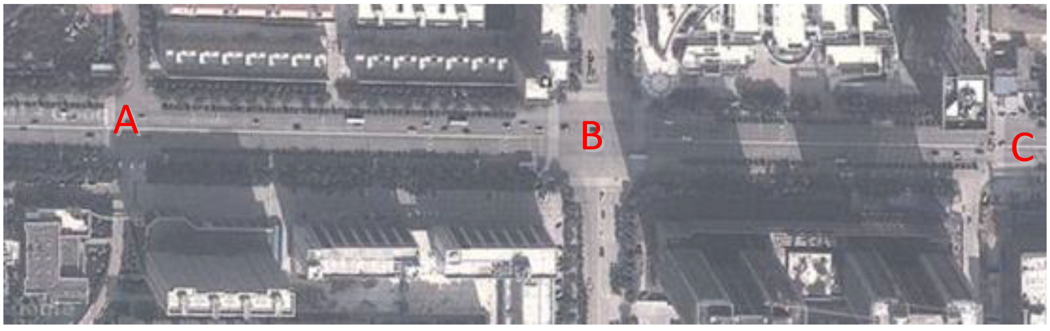
In this section, the proposed model and method are applied to a real example, which is three consecutive intersections in a main road of Baoji city. Figure 2 shows the layout of the three intersections.

This study collected 24-h traffic flow data at three intersections through artificial investigation, video capture, and coil detector. Corresponding traffic volume-time curves are shown in Figure 3, from which can be seen the variations of traffic flow at the three intersections tend to be the same. There are two main peak periods of the day, with the morning peak at 7:30–8:30 and the evening peak at 18:00–19:00. In contrast, during the evening peak hour, the peak flow is more prominent, the distribution of traffic arrivals is more regular, and no flow anomalies occur, which meets the research requirements. In order to improve the accuracy of the analysis results, the data collected should be continuous and correlated. Thus, three consecutive hours (16:30–19:30) were selected as the analysis period, and the various data collected were used as the basis for the case analysis.

In addition, the average queue length, the delay and the saturation are selected to construct an evaluation system. The three indicators are calculated as follows:

(1) The calculating process of average delay

The data collected by the point sample method are used to calculate the average delay. Taking a one-way lane at an intersection as an example, the basic steps of data collection are as follows:

①

Observer A counts the number of vehicles parked behind the stop line every 15 s.

②

Observer B counts the number of vehicles passing the stop line after parking (number of stopped vehicles) and the number of passing the parking line without stopping (number of non-stopped vehicles) at 1-min intervals.

③

Repeat the above process to obtain the data for the survey time period.

The calculation can be conducted as follows:

$$D_{sum}=N_1*t_0$$

(21)

$$d_s=D_{sum}/N_2$$

(22)

$$d_i=D_{sum}/(N_2+N_3)$$

(23)

(2) The calculating process of average queue length

Record the numbers of different types of vehicles in the queue of each signal cycle $n_j^i$, then the average queue length can be calculated as:

$$aql=\frac{n_v^c\cdot l_v}{k}$$

(24)

(3) The calculating process of average saturation

This indicator can be calculated based on the ratio between the capacity and the actual volume. Taking the one-way entrance lane of an intersection as an example, the number of vehicles passing through the lane in a unit time can be collected during the study period and the capacity of the lane can be calculated. By repeating the above process, average saturation data for each direction and the entire intersection can be obtained. The calculation of this indicator is a basic part of the data survey and the details presented in the literature [42].

Based on the calculation process presented above, the data of the three intersections including the queue, the delay and the saturation degree are obtained during the analysis period (16:30–19:30), as shown in

Table 2. The traffic data of the three intersections.

Intersection A
No.	Time Period	Average Queue Length (m)	Average Delay (s)	Average Saturation Degree (%)
$T_1$	16:30–17:30	16.69	26.37	81.65
$T_2$	17:30–18:30	21.46	29.43	93.24
$T_3$	18:30–19:30	27.62	32.2	107.02
Intersection B
No.	Time Period	Average Queue Length (m)	Average Delay (s)	Average Saturation Degree (%)
$T_1$	16:30–17:30	11.29	21.42	69.03
$T_2$	17:30–18:30	16.57	26.68	81.46
$T_3$	18:30–19:30	23.89	30.31	90.79
Intersection C
No.	Time Period	Average Queue Length (m)	Average Delay (s)	Average Saturation Degree (%)
$T_1$	16:30–17:30	17.23	25.51	90.76
$T_2$	17:30–18:30	24.39	34.47	103.69
$T_3$	18:30–19:30	32.08	40.12	118.37

.

Based on the data, the risk degree of the three intersections can be derived from the model calculation. Accordingly, some measures of traffic management and control to reduce the risk are given. The detailed calculation process of the model is as follows:

Step 1: Constructing the initial decision matrix.

The values of the three indicators of queue length, average delay and saturation, are initialized on three intersections between 16:30 and 19:30. Each hour is considered as a time-point, and the value of the indicator in each time period provides the information for the time-point. According to Equations (1) and (2), the data in Table 2 are transformed into the risk-free decision matrix.

The risk-free decision matrix of intersection A is

$$E_1=\left[\left[\begin{array}{ccc}0.591& 0.611& 0.632\\ 0.613& 0.635& 0.722\\ 0.595& 0.632& 0.618\end{array}\right]\left[\begin{array}{ccc}0.623& 0.780& 0.705\\ 0.555& 0.615& 0.715\\ 0.568& 0.653& 0.699\end{array}\right]\left[\begin{array}{ccc}0.585& 0.613& 0.615\\ 0.603& 0.645& 0.702\\ 0.621& 0.687& 0.699\end{array}\right]\right]$$

The risk-free decision matrix of intersection B is

$$E_2=\left[\left[\begin{array}{ccc}0.602& 0.671& 0.619\\ 0.651& 0.605& 0.723\\ 0.665& 0.678& 0.701\end{array}\right]\left[\begin{array}{ccc}0.573& 0.601& 0.605\\ 0.625& 0.785& 0.718\\ 0.589& 0.603& 0.698\end{array}\right]\left[\begin{array}{ccc}0.594& 0.601& 0.653\\ 0.583& 0.585& 0.672\\ 0.605& 0.698& 0.699\end{array}\right]\right]$$

The risk-free decision matrix of intersection C is

$$E_3=\left[\left[\begin{array}{ccc}0.518& 0.621& 0.633\\ 0.513& 0.525& 0.672\\ 0.573& 0.568& 0.605\end{array}\right]\left[\begin{array}{ccc}0.621& 0.665& 0.677\\ 0.564& 0.567& 0.671\\ 0.527& 0.662& 0.633\end{array}\right]\left[\begin{array}{ccc}0.625& 0.618& 0.609\\ 0.661& 0.625& 0.710\\ 0.651& 0.624& 0.687\end{array}\right]\right]$$

After converting the information of all time-points to a risk-free decision-making matrix, a standardized processing should be conducted to reduce the negative effect that different dimensions have on the decision making. According to Equations (3) and (4), the standard decision matrix of the three intersections can be derived through normalizing the corresponding risk-free decision matrix.

The standard decision matrix of intersection A is

$$Y_1=\left[\left[\begin{array}{ccc}0.312& 0.315& 0.307\\ 0.323& 0.325& 0.402\\ 0.355& 0.432& 0.418\end{array}\right]\left[\begin{array}{ccc}0.223& 0.217& 0.331\\ 0.305& 0.316& 0.317\\ 0.218& 0.313& 0.309\end{array}\right]\left[\begin{array}{ccc}0.225& 0.323& 0.345\\ 0.303& 0.325& 0.328\\ 0.311& 0.317& 0.339\end{array}\right]\right]$$

The standard decision matrix of intersection B is

$$Y_2=\left[\left[\begin{array}{ccc}0.325& 0.337& 0.339\\ 0.253& 0.255& 0.332\\ 0.255& 0.322& 0.308\end{array}\right]\left[\begin{array}{ccc}0.313& 0.307& 0.401\\ 0.225& 0.236& 0.267\\ 0.227& 0.332& 0.314\end{array}\right]\left[\begin{array}{ccc}0.235& 0.331& 0.315\\ 0.306& 0.315& 0.317\\ 0.391& 0.305& 0.308\end{array}\right]\right]$$

The standard decision matrix of intersection C is

$$Y_3=\left[\left[\begin{array}{ccc}0.303& 0.333& 0.336\\ 0.268& 0.306& 0.326\\ 0.353& 0.373& 0.383\end{array}\right]\left[\begin{array}{ccc}0.233& 0.236& 0.331\\ 0.239& 0.313& 0.333\\ 0.238& 0.331& 0.334\end{array}\right]\left[\begin{array}{ccc}0.229& 0.321& 0.324\\ 0.322& 0.325& 0.329\\ 0.322& 0.324& 0.326\end{array}\right]\right]$$

Step 2: Determining the weighted standard decision matrix.

After a dimensionless process, a standard decision matrix is obtained for the three intersections. As a basis for the subsequent calculations, it is necessary to determine the weighting vector to obtain a weighted decision matrix for the three intersections. The attribute weights $W_j$ corresponding to indicator $C_j$, including queue length, average delay and saturation can be calculated by Equations (5)-(8), which reflects the influence on the risk level evaluation results of traffic congestion at the case intersection. By using the standard deviation method, the weight coefficients of the three evaluation indicators can be calculated and the results are as follows:

$$\stackrel{\rightharpoonup }{W}=(0.327,0.332,0.341)$$

According to Equation (9), the weighted standard decision matrix can be obtained as follows:

$$B=\left[\left[\begin{array}{ccc}0.212& 0.232& 0.262\\ 0.223& 0.227& 0.229\\ 0.222& 0.225& 0.228\end{array}\right]\left[\begin{array}{ccc}0.223& 0.226& 0.229\\ 0.224& 0.223& 0.228\\ 0.223& 0.226& 0.230\end{array}\right]\left[\begin{array}{ccc}0.235& 0.237& 0.331\\ 0.232& 0.235& 0.239\\ 0.232& 0.234& 0.236\end{array}\right]\right]$$

Step3: Determining the positive and negative decision matrix and calculating the relevancy of intersection congestion.

The weight vector for different time-points depends on the change in the values of each indicator at the three intersections at different time-points. The weight vector of time-points can be obtained by using the three-scale method.

$$\stackrel{\rightharpoonup }{\lambda }=(0.313,0.352,0.335)$$

Based on the weight vector at each time-point, the standardized matrix sequence $Y_i$ about the time-points can be converted into a matrix sequence $H_k$ about the decision solution $X_k$ according to Equation (15). $H_k$ is also known as the integrated decision solution matrix, which represents the level of traffic congestion risk at each intersection. For each decision matrix, there is a positive ideal matrix $F$ and a negative ideal matrix $G$. According to Equations (10) and (11), the positive ideal matrix and the negative ideal matrix of the intersection congestion can be obtained, respectively.

$$F=\left[\left[\begin{array}{ccc}0331& 0.336& 0.339\\ 0.333& 0.335& 0.337\\ 0.335& 0.337& 0.339\end{array}\right]\left[\begin{array}{ccc}0.332& 0.336& 0.341\\ 0.335& 0.337& 0.339\\ 0.333& 0.336& 0.339\end{array}\right]\left[\begin{array}{ccc}0.325& 0.327& 0.329\\ 0.322& 0.325& 0.341\\ 0.325& 0.327& 0.329\end{array}\right]\right]$$

$$G=\left[\left[\begin{array}{ccc}0.221& 0.223& 0.225\\ 0.221& 0.223& 0.227\\ 0.222& 0.223& 0.225\end{array}\right]\left[\begin{array}{ccc}0.233& 0.236& 0.238\\ 0.231& 0.233& 0.235\\ 0.233& 0.235& 0.237\end{array}\right]\left[\begin{array}{ccc}0.241& 0.243& 0.245\\ 0.242& 0.245& 0.247\\ 0.242& 0.244& 0.245\end{array}\right]\right]$$

The correlation between the decision matrix and the positive/negative ideal matrices is then analyzed, through which the validity of the decision scheme can be evaluated and the congestion risk of the intersection can be judged. According to Equations (13) and (14), the correlation degree of the decision matrix $H_k$ with the decision positive ideal matrix $F$ and negative ideal matrix G was calculated for the three intersections as follows:

$$[{\overline{\overline{R}}}_1^{(+)}]=\gamma (\stackrel{\approx }{F},{\stackrel{\approx }{H}}_1)=0.6821,[{\overline{\overline{R}}}_1^{(-)}]=\gamma (\stackrel{\approx }{G},{\stackrel{\approx }{H}}_1)=0.5746$$

$$[{\overline{\overline{R}}}_2^{(+)}]=\gamma (\stackrel{\approx }{F},{\stackrel{\approx }{H}}_2)=0.8549,[{\overline{\overline{R}}}_2^{(-)}]=\gamma (\stackrel{\approx }{G},{\stackrel{\approx }{H}}_2)=0.3651$$

$$[{\overline{\overline{R}}}_3^{(+)}]=\gamma (\stackrel{\approx }{F},{\stackrel{\approx }{H}}_3)=0.4584,[{\overline{\overline{R}}}_3^{(-)}]=\gamma (\stackrel{\approx }{G},{\stackrel{\approx }{H}}_3)=0.8614$$

According to the definition of correlation degree, the decision scheme of intersection B has the highest correlation with the positive ideal scheme and the lowest correlation with the negative ideal scheme, which indicates that intersection B faces the lowest level of risk of traffic congestion.

Step 4: Calculating the subordinate degree and risk sorting.

The risk of traffic congestion at the three intersections should be judged more precisely. According to Equations (18)–(20), the subordinate degree of the three intersections can be calculated, respectively.

$$[{\overline{\overline{u}}}_1]=0.5849,[{\overline{\overline{u}}}_2]=0.8457,[{\overline{\overline{u}}}_3]=0.2207$$

According to the specific sorting rule of risk identification, the calculation results of subordinate degree of the three intersections are sorted in a descending order:

$$[{\overline{\overline{u}}}_2]>[{\overline{\overline{u}}}_1]>[{\overline{\overline{u}}}_3]$$

Thereby the risk degree of the three intersections can be obtained as:

Intersection C > Intersection A > Intersection B

The sorted result indicates that the intersection C has the highest risk of traffic congestion and the intersection B has the lowest risk. The evaluation results are in accord with the actual condition since there are shopping malls and office buildings around the intersection C, which has brought a very large additional traffic demand compared with intersection A and B. The traffic congestion in intersection C is mainly caused by the car travel demand exceeding the traffic capacity. To avoid this problem, some measures of traffic planning and management should be implemented in intersection C, including improving the traffic capacity of intersections by widening the key approaches and reducing the car travel demand by adding the bus exclusive lane to the existing road.

6. Conclusions

With the acceleration of urbanization, traffic congestion has become more and more serious, which leads to longer travel times and limited reliability of the transportation and causes high energy consumption and emission. So, the research on the traffic congestion problem is of important practical significance. In this paper, we proposed a new methodology to identify and predict the risk degree of intersection congestion by taking into consideration the traffic flow’s intrinsic properties and the traffic congestion model. First, an integrated evaluation index system was constructed, in which some congestion factors have been taken as the core indicators to evaluate the risk degree of the intersection congestion. Then, based on the risk identification theory, a detailed dynamic decision model of the road intersection congestion was presented, which can be used to identify the risk degree of intersection congestion and predict its influence on future traffic flow. Finally, the proposed approach was applied to a real case in Baoji city.

The application results showed that the dynamic decision model can not only reflect the actual traffic condition of the intersection, but also predict the spread trend of traffic congestion, by which the traffic management and control measures can be taken in real-time to reduce the original congestion point. So, the presented approach is a practical, effective and feasible way to alleviate the traffic congestion, which can be used as a tool to help transport planners change the traffic planning schemes as well as help transport managers make some management and control measures in advance while considering a network perspective.

However, caution should be taken while directly referring to this conclusion and several extensions may be considered in future work. First of all, during model construction, only three indicators including queuing length, average delay and saturation degree, are selected as the decision indicators of the model, which are all used to reflect the operation efficiency of intersection. That, however, may affect the accuracy of the evaluation results. Future research would consider incorporating more indicators relating to traffic capacity and service level into the dynamic decision model, so that the accuracy of evaluation results can be further improved. Secondly, this paper is focused on the objective empowerment idea to determine the weight values of the decision indicators. The approach relies on objective criteria for empowerment and ignores information about the decision-maker’s preferences such as knowledge and experience. It fails to reflect the importance of different attribute indicators to the decision-maker and may lead to unreasonable weighting. In future, it is possible to consider the integration of subjective and objective empowerment methods, such as integrating the existing subjective and objective weight information into the cloud model to form a cloud portfolio empowerment method. In this way, the subjective judgment of the decision- maker and the objective characteristics of the evaluation object are taken into account. It solves the problem of ambiguity and randomness in the process of weight combination and improves the validity and reasonableness of the results. Finally, the proposed approach considers the intersection as an isolated entity and lacks capturing the spatial dependence between different intersections. As a result, the evaluation approach may not work well in the case that several consecutive intersections are contained. The upstream link has a positive impact on the traffic conditions of the interest link, which needs to be incorporated in the process of establishing the model. In future research, the spatial dependence structure between traffic links should be predefined and embedded in the model.

References

1. Vlahogianni, E.I.; Karlaftis, M.G.; Kepaptsoglou, K. Nonlinear autoregressive conditional duration models for traffic congestion estimation. J. Probab. Stat. 2011, 2011, 1–13. [Google Scholar] [CrossRef] [Green Version]
2. Min, W.; Wynter, L. Real-time road traffic prediction with spatio-temporal correlations. Transp. Res. Part C Emerg. Technol. 2011, 19, 606–616. [Google Scholar] [CrossRef]
3. Alireza, E.; David, L. Spatiotemporal traffic forecasting: Review and proposed directions. Transp. Rev. 2018, 38, 786–814. [Google Scholar] [CrossRef]
4. Michalopoulos, P.G.; Pisharody, V.B. Derivation of delays based on improved macroscopic traffic models. Transp. Res. Part B Methodol. 1981, 15, 299–317. [Google Scholar] [CrossRef]
5. Morales, J.M. Analytical procedures for estimating freeway traffic congestion. Public Roads 1987, 51, 55–61. [Google Scholar]
6. Newell, G.F. A simplified theory of kinematic waves in highway traffic, part I: General theory. Transp. Res. Part B Methodol. 1993, 27, 281–287. [Google Scholar] [CrossRef]
7. Zambrano, M.J.L.; Calafate, C.T.; Soler, D.; Cano, J.C.; Manzoni, P. Modeling and characterization of traffic flows in urban environments. Sensors 2018, 18, 2020. [Google Scholar] [CrossRef] [Green Version]
8. Sheu, J.B. A fuzzy clustering-based approach to automatic freeway incident detection and characterization. Fuzzy Sets Syst. 2002, 128, 377–388. [Google Scholar] [CrossRef]
9. Fu, L.; Hellinga, B.; Zhu, Y. An adaptive model for real-time estimation of overflow queues on congested arterials. IEEE Intell. Transp. Syst. 2001, 219–226. [Google Scholar] [CrossRef]
10. Wen, H.M. The Research on the Key Theory and Technology of the Traffic Congestion in Highway. Ph.D. Thesis, University of Jilin, Jilin, China, 2002. (In Chinese). [Google Scholar]
11. Zang, H.; Peng, G.X. The prediction model of queue length under the abnormal condition in highway. J. Transp. Inf. Saf. 2003, 21, 10–12. (In Chinese) [Google Scholar]
12. Peng, C.L.; Yang, X.G.; Zhang, C.B. Character of traffic flow in queue upstream of bottleneck based on I/O. J. Transp. Inf. Saf. 2004, 12, 1–4. (In Chinese) [Google Scholar]
13. Jiang, G.Y.; Dai, L.L.; Bai, Z.; Zhao, J.Q.; Zhen, Z.T. Simulation of recurrent congestion diffusion of urban arterial street. J. Transp. Inf. Saf. 2006, 24, 1–3. (In Chinese) [Google Scholar]
14. Juran, I.; Prashker, J.N.; Bekhor, S.; Ishai, I. A dynamic traffic assignment model for the assessment of moving bottlenecks. Transp. Res. Part C Emerg. Technol. 2009, 17, 240–258. [Google Scholar] [CrossRef]
15. Lawson, T.W.; Lovell, D.J.; Daganzo, C.F. Using input-output diagram to determine spatial and temporal extents of a queue upstream of a bottleneck. Transp. Res. Rec. 1997, 1572, 140–147. [Google Scholar] [CrossRef] [Green Version]
16. Hu, Q.Z.; Liu, Y.S.; Tang, G.Y. Space-Time distribution model on state monitoring of urban traffic congestion. J. Transp. Syst. Eng. Inf. Technol. 2013, 12, 41–45. (In Chinese) [Google Scholar]
17. Liu, Y.J.; Tian, C. Analysis of dynamic characteristics of urban traffic congestion based on specificity of network configuration. China J. Highw. Transp. 2013, 26, 163–169. (In Chinese) [Google Scholar]
18. Hu, L.W.; Yang, J.Q.; He, Y.R.; Meng, L.; Lou, Z.W.; Hu, C.Y. Urban traffic congestion radiation model and damage caused to service capacity of road network. China J. Highw. Transp. 2019, 32, 145–154. (In Chinese) [Google Scholar]
19. Van Zuylen, H.J.; Viti, F. Delay at controlled intersections: The old theory revised. In Proceedings of the IEEE Intelligent Transportation Systems Conference, Toronto, ON, Canada, 17–20 September 2006; pp. 68–73. [Google Scholar] [CrossRef]
20. Liu, H.X.; Wu, X.; Ma, W.; Hu, H. Real-time queue length estimation for congested signalized intersections. Transp. Res. Part C Emerg. Technol. 2009, 17, 412–427. [Google Scholar] [CrossRef]
21. Chang, Y.L.; Cui, Y.B.; Zhang, P. Multi-phase signal setting and capacity of signalized intersection. J. Southeast Univ. 2009, 25, 123–127. (In Chinese) [Google Scholar]
22. Zheng, F.F.; Van Zuylen, H. Uncertainty and predictability of urban link travel time: Delay distribution–based analysis. Transp. Res. Rec. 2010, 2192, 136–146. [Google Scholar] [CrossRef]
23. Lin, P.Q.; Zhuo, F.Q.; Yao, K.B.; Rang, B.; Xu, J.M. Solving and simulation of microcosmic control model of intersection traffic flow in connected-vehicle network environment. China J. Highw. Transp. 2015, 28, 82–92. (In Chinese) [Google Scholar]
24. Xu, J.M.; Yan, X.W.; Jing, B.B.; Wang, Y.J. Dynamic network partitioning method based on intersections with different degree of saturation. J. Transp. Syst. Eng. Inf. Technol. 2017, 17, 145–152. (In Chinese) [Google Scholar]
25. Zhao, J.; Zhen, Z.; Han, Y. Delay and optimal cycle length model for tandem intersections. China J. Highw. Transp. 2019, 32, 135–144. (In Chinese) [Google Scholar]
26. Yu, Z.; Huang, L.H.; Li, X.Y.; Li, B.; Zou, B. Queueing process sensing and prediction at intersection based on video. J. Transp. Syst. Eng. Inf. Technol. 2020, 20, 33–39. (In Chinese) [Google Scholar]
27. Yang, D.; Chen, Y.; Xin, L.; Zhang, Y. Real-time detecting and tracking of traffic shockwaves based on weighted consensus information fusion in distributed video network. IEEE Intell. Transp. Syst. 2013, 8, 377–387. [Google Scholar] [CrossRef]
28. He, Z.; Qi, G.; Lu, L.; Chen, Y. Network-wide identification of turn-level intersection congestion using only low-frequency probe vehicle data. Transp. Res. Part C Emerg. Technol. 2019, 108, 320–339. [Google Scholar] [CrossRef]
29. Li, S.; Li, G.; Cheng, Y.; Ran, B. Intersection congestion analysis based on cellular activity data. IEEE Access 2020, 8, 43476–43481. [Google Scholar] [CrossRef]
30. Xia, X.; Deng, W.; Hu, Q.Z. Research on interval-number evaluation method and solutions for traffic congestion in urban road sections. J. Transp. Syst. Eng. Inf. Technol. 2007, 17, 121–125. (In Chinese) [Google Scholar]
31. Su, F.; Dong, H.; Jia, L.; Sun, X. On urban road traffic state evaluation index system and method. Mod. Phys. Lett. B 2017, 31, 1650428. [Google Scholar] [CrossRef]
32. Zhang, P.; Zhao, J.; Wang, Z.Y.; An, H.S.; Peng, S. Overall evaluation of signal controlled intersection based on Monte Carlo simulation. J. Heilongjiang Inst. Technol. 2013, 327, 1–5. (In Chinese) [Google Scholar]
33. Chen, K.M.; Yan, B.J. Analysis of Road Traffic Capacity; People Communications Publishing House: Beijing, China, 2003; pp. 188–190. [Google Scholar]
34. Hao, N.; Feng, Y.; Zhang, K.; Tian, G.; Zhang, L.; Jia, H. Evaluation of traffic congestion degree: An integrated approach. Int. J. Distrib. Sens. Netw. 2017, 13, 1–14. [Google Scholar] [CrossRef] [Green Version]
35. Zhu, Q.; Hui, L.; Xia, G.; Yu, M. Dynamic multi-attribute decision making of carrier-based aircraft landing risk. J. Harbin Eng. Univ. 2013, 34, 616–622. (In Chinese) [Google Scholar]
36. Qing, L.Z.; Ye, Q.G. A new grey incidence model of interval numbers and its application. In Proceedings of the 2011 IEEE International Conference on Systems Man, and Cybernetics, Anchorage, AK, USA, 9–12 October 2011; pp. 1881–1885. [Google Scholar] [CrossRef]
37. Wang, X.; Xie, K.; Abdel-Aty, M.; Chen, X.; Tremont, P.J. Systematic approach to hazardous-intersection identification and countermeasure development. J. Transp. Eng. 2014, 140, 04014022. [Google Scholar] [CrossRef] [Green Version]
38. Zhao, N.; Wei, C.P.; Bi, Y.Z. Determining expert weights and its sensitivity analysis based on the correlation coefficient and the standard deviations. J. Qufu Norm. Univ. 2013, 39, 25–32. (In Chinese) [Google Scholar]
39. Xu, Y.J.; Da, Q.L. Standard and mean deviation methods for linguistic group decision making and their applications. Expert Syst. Appl. 2010, 37, 5905–5912. [Google Scholar] [CrossRef]
40. Wang, Z.X.; Shao, C.L.; Tang, Z.L. Method for ranking interval numbers based on relative superiority and its application to multiple attribute decision making. Fuzzy Syst. Math. 2013, 27, 142–148. (In Chinese) [Google Scholar]
41. Sengupta, A.; Pal, T.K. On comparing interval numbers: A study on existing ideas. Fuzzy Prefer. Ord. Interval Numbers Decis. Probl. 2009, 2, 25–37. [Google Scholar] [CrossRef]
42. Sun, C. Research on Urban Traffic Network State Evaluation and Analysis. Master’s Thesis, South China University of Technology, Guangzhou, China, 2010. [Google Scholar]
Figure 1. The evaluation index system of the intersection congestion.
Sustainability 12 05923 g001
Figure 2. The layout of the three intersections.
Sustainability 12 05923 g002
Figure 3. The traffic volume-time distribution of the three intersections.
Sustainability 12 05923 g003