Article

Soil-Based Vegetation Productivity Model for Coryell County, Texas

1
College of Landscape Architecture and Art, Hunan Agriculture University, Changsha 410128, China
2
College of Landscape Architecture, Beijing Forestry University, Beijing 100083, China
3
Landscape Architecture, School of Planning, Design, and Construction, Michigan State University, East Lansing, MI 48824, USA
*
Author to whom correspondence should be addressed.
Sustainability 2020, 12(13), 5240; https://doi.org/10.3390/su12135240
Submission received: 29 April 2020 / Revised: 14 June 2020 / Accepted: 18 June 2020 / Published: 28 June 2020
(This article belongs to the Special Issue Sustainable Environmental Reclamation: Landscape Planning and Design)

Abstract

:
Managers, scientists, planners and designers of landscapes are interested in systematic investigations, to predict the reconstruction of disturbed soil resources for optimum vegetation productivity. In this study, a predictive equation for estimating neo-soil plant growth in Coryell County, Texas was developed. The equation predicts the vegetation growth for wheat (Triticum aestivum L.), oats [Avena sativa L. (1753)], sorghum [Sorghum bicolor (L.) Moench], cotton lint (Gossypium hirsutum L.), Bermuda grass [Cynodon dactylon (L.) Pers.], and rangeland production in general. The results suggest that an all-vegetation predictive model was highly significant (p ≤ 0.0001), explaining over 80% of the variance. The equation employed hydraulic conductivity as a main-effect variable; bulk density and hydraulic conductivity as squared terms; and percent clay times bulk density, bulk density times soil reaction, hydraulic conductivity times available water holding capacity, and hydraulic conductivity times soil reactions as first order interaction terms, with each predicting variable containing a p-value equal to or less than 0.05. The results suggest that an annual crop equation and a plant-specific cotton lint equation also have merit.

1. Introduction

Since the 1980s, reclamation scientists have urged the development of science-based equations to predict plant growth in soils [1,2,3]. The call was made because native soils were being disturbed (at the time by surface mining, but also as a consequence of urban sprawl, transportation corridors and facilities, and general effects of human activity on the planet). The reconstructed soil required assessment, as it rarely resembled the native soils previously residing upon the site. In the United States, private soil testing companies, universities and county government cooperatives test soil for soil texture, soil nutrient recommendations and engineering properties, for construction purposes. The intention and call for soil productivity equations paralleled these existing tests, as it was believed that soil productivity equations could be added to the palette of available tests pertinent to soil metrics and properties, especially in surface mine reclamation, but also with regards to the vast array of human activities that reconstruct the soil profile.
The typical approach was to construct a new soil (neo-sol) profile, and then grow crops on the new profile to determine the soil’s productivity, comparing the productivity with past productivity or to current reference areas. However, this takes time, often up to 10 years of evaluation. There are wet years, dry years, insect infestations, diseases, and varying spatial environmental conditions (such as heavy rainfall in one area, and no rainfall at all just 500 m away). Thus, it often took a decade of average soil productivity values to estimate actual productivity. After 10 years, if the soil was found to be less productive (defective), often little could be done to offer extensive modifications to the soil profile. Government agencies could commandeer mining company reclamation bonds (bonds posted to ensure the reclamation and protection of land-owners’ and government land), but even with the money, it was difficult to amend the soil profile. In addition, the mining company waiting a decade for the release of a bond was an expensive proposition. It was believed that with the development of reliable reclamation equations, one could predict soil productivity by taking measurements of the soil profile and plugging them into an equation within days, eliminating years of waiting. In the mined land reclamation process, these equations might also assist in developing profiles and design alternatives to efficiently and effectively utilize soil properties and resources, to maximize/optimize post-mining productivity. This call for the equations existed long before much of the population was strongly interested in sustainability, at a time when citizen environmental activists, concerned politicians and natural resource scientists passionate about such issues were still a small minority.
The task to produce these equations seemed difficult because many questions remained. How many equations for how many different plants were necessary? Which soil properties were most suited to predict plant growth, and from where in the soil profile were they to be measured? The answers to these questions were resolved by Burley and Thomsen in 1987, and reiterated by Burley in 1996 [3,4]. Essentially, the findings suggested that principal component analysis (PCA) could resolve how many equations were necessary, and that soil scientists had identified the 10 most likely soil variables most useful in predictive modeling: topographic position, percent slope, percent organic matter, percent rock fragments, available water holding capacity, soil reaction, hydraulic conductivity, bulk density, electrical conductivity and percent clay. In addition, soil scientists had discovered that the first four feet (1.2192 m) of the soil profile would suffice in the analysis, with the first foot (30.48 cm) of the profile contributing 40% towards plant growth, the second 30.48 cm 30%, the third 30.48 cm 20%, and the fourth 30.48 cm 10% [3,4]. Providing that crops were grown and their growth recorded across numerous measured soil profiles, an equation could be constructed [3,4]. The data for such analysis could be found in the United States Department of Agriculture soil surveys, starting in the very late 1890s and early 1900s, with numerous updates, revisions and additions [5,6]. The statistical concept for conducting this type of research was proposed by Kendal in 1939, so this approach to predicting vegetation productivity has been long in the making, and has been slowly evolving [7].
In this type of study, there are always other soil property variables, such as soil organism biodiversity indexes or other properties, that could be used [8,9]. Those who study these properties will be staunch defenders of such variables, indicating the importance and value of such variables. It would be highly useful to have the soil surveys updated with the values for these variables in each soil profile, to advance the state of the art in constructing these models. Much has been learned about soil properties and soil productivity since the initial early survey studies were published. The updating of these soil surveys is highly valuable, adding other crop productivity values and soil parameters for a more informed data set. With the advent of digital communications, attachments, and appendices to current pdf reports published on internet databases, the effort can be efficiently accomplished. The United States Department of Agriculture recognizes this issue/opportunity, and has pursued updates in its soil survey databases, such as in 2018, when it added suitability interpretations for aerobic soil organisms, agricultural organic soil subsidence, concentration of soil surface salts, organic matter depletion, soil surface sealing, catastrophic event—large animal mortality—burial, catastrophic event—large animal mortality—incineration, natural surface road construction and maintenance, displacement hazard, puddling hazard, compatibility risk, and windthrow hazard [10]. Given that the proposed predictors for reclamation modeling were identified in the mid-1980s by a team in North Dakota, it may be a worthwhile venture for the soil reclamation/soil science academic community to readdress the list of potential regressors associated with vegetation productivity [3,4]. While measures such as the soil organism biodiversity index could be a potential regressor to predict vegetation productivity, it may also constitute a dependent variable, where other soil parameters combine to predict soil organism biodiversity, and covary with vegetation productivity, forming a network/web as opposed to simply a set of independent and dependent variables.
To produce the detailed soil surveys, the Natural Resource Conservation Service (NRCS), formerly the Soil Conservation Service (SCS), grows numerous crops across numerous measured soil profiles, and provides a county by county data set. Each data set takes about 10 years to prepare, and often over one million American dollars (in 1980’s American dollars) to construct [3,4]. These data sets are quite comprehensive, with detailed maps for each county studied. Most of the county data and maps were produced for American agricultural areas, and financed by the Federal government [6,9]. Much of the American landscape still has not been assessed and mapped, especially in mountainous areas [9]. While some of these data sets are over 60 years old, they remain the most detailed and reliable sets of soil productivity, and are extensively used by farmers and county agents today. They only become dated when urban sprawl overtakes an area, or when the land is disturbed by mining or another form of disturbance, changing the soil profile. Since these maps and data sets are expensive to construct, many/most parts of the world have yet to create such detailed information sets about their landscapes. Many countries do not have the financial resources to collect such detailed information about their agricultural and forested lands. “I have been invited to Asian and European countries to discuss how to produce the data necessary to statistically derive soil productivity equations. Most of the time colleagues are quite impressed with the American initiative.” states Dr. Burley. “But when confronted with the cost and time necessary to make such a study, several millions in American dollars or equivalent per 300,000 to 400,000 hectares, the effort seems too difficult to achieve. Most academic research projects only have a two or three year cycle and may be only at most several hundred thousand American dollars in cost. Spending 30 years and hundreds of millions of dollars to develop a detailed national data set is beyond the time-frame or financial resources for many countries and research agendas. Thus the American data set is somewhat special, reflective of a wealthy nation, and a Federal government focused upon the long-term. In many places around the world, there is pressure for modest spending and immediate research results that cannot match what the Americans achieved, especially during the post World War II era. I am doubtful if the Americans were just starting upon such a research endeavor, they would have achieved the same comprehensive and expansive data set that now exists. It is too easy for politicians to cut the funding of projects initiated by predecessors, seeking immediate results that fit the timing of re-election cycles. This is an unfortunate reality for anyone interested in science and sustainability issues. In addition, I have encountered international governmental and business groups interested in making a quick and lucrative profit from advanced agricultural techniques, as opposed to maintaining the health of disturbed soils. On the other hand, I have met farmers who intimately know their soil and land, taking a long term perspective in managing the soil resources.”
With the American data sets, the first reported equations employing this information were reported for Clay County Minnesota, by Burley, Thomsen and Kenkel [11,12,13]. They discovered that most grown crops and woody plants grown in the study area preferred the same soil characteristics. This is known as the “Mesic Soil Vegetation Preference Theory.” This was an important finding. Before this time, there was much debate concerning the number of equations necessary to predict vegetation productivity. The Mesic Soil Vegetation Preference Theory and statistical results (model) suggested that many plants preferred that same soil. In addition, for the Clay County study area, sugar beet (Beta vulgaris L.) could be expressed in its own equation [14]. Sugar beets could grow in more saline, wet, poorly aerated, and poor-draining soils, such as those found in post-glacial lake bottoms, like in the Red River Valley of the north (the area of glacial Lake Agassiz, a lake that deposited up to 150 m of clay).
In 1993, Burley and Bauer reported two equations for Polk County, Florida [15]. Polk County is an area disturbed by massive phosphate mining, where reclamation soil productivity equations could be helpful. The post-mining landscape would be composed of groves of orange tree [Citrus x sinensis (L.) Osbeck] plantations, housing, and recreation open space containing wetlands. In the study, one equation was for mesic-seeking plants, and the other for hydric seeking vegetation. This led to the “Hydric Soil Vegetation Preference Theory.” In the warm and wet subtropical areas of the United States, it appeared there were broadly two distinct groups of plants, preferring two different characteristics in soil profiles.
So far, only areas in the range of 300,000 to 400,000 hectares in size had been evaluated. In 1995, Burley reported the first multi-county model for Clay County Minnesota and Cass County, North Dakota [16]. A three-country model (over 1,000,000 hectares) was studied for the coal mining region of North Dakota, reporting various equations [17,18]. Practical spatial applications of the equations were reported in 1999 [19]. By 2001, a study reporting the relationship of these “softscape” soils (for vegetation) and “hardscape” soils (for buildings, roads and plazas) was explored, suggesting there were some types of soils that were suitable for both, but that most of these soils were exclusively useful for either softscapes or hardscapes [20]. These studies, along with practical planning and design illustrations for various land-uses, led to the publication of Environmental Design for Surface Mine Reclamation, a publication that earned state and national American Society of Landscape Architects awards [21]. Much of this early literature was published in conference proceedings in the surface mining reclamation arena, as this was the common academic venue for reporting this research by American academics. Over time, the emergence of reclamation journals, such as the America Society for Mining and Reclamation (now the American Society of Reclamation Sciences), and the scholarly drift towards and emphasis upon journal publication, has led to a different approach in reporting the results of these equations. Now, the same conference proceedings are published in their journal.
Slowly, equations for other counties across the eastern United States were reported. A French and American team reported an equation for Traverse County in Michigan, an area disturbed by recreational housing and general development [22]. Equations were reported for Chippewa County in Wisconsin (an area mined for silica sand to make glass) and for an area in Georgia (an area mined for sand and gravel and for kaolin clay) by a Chinese and American team [23,24]. These two studies supported similar equations, reinforcing the Mesic Preference Theory for mid-continent temperate areas with adequate moisture for vegetation.
Recently, another Chinese and American team reported upon equations in the coal mining regions of Montana, Wyoming and Colorado [25]. The study in Montana, Wyoming and Colorado revealed differences in the equations concerning high altitude and crop production in extremely cold and dry environments. The focus was still primarily on supporting surface mine reclamation, and the study was conducted primarily through the efforts of one American scientist, devoted to studying soil productivity equations, graduate students, and international scholars interested in the methodology, which earned the American scholar the American Society of Reclamation Sciences researcher of the year award. In surface mining reclamation circles, the research is well received and modestly known, but not widely pursued by others. Yet, as each region is studied and reported, it adds to the knowledge of the similarities and difference in soil productivity across the eastern 3/5ths of the United States.
There may be several reasons why the methodology may not yet be widely examined by others. First, the equations are lengthy and complex, introducing previously-unstudied relationships between soil properties. The statistical interactions of soil parameters that predict soil productivity may perplex investigators, and challenge normative beliefs concerning soil productivity. To validate and understand these equations and interactions may require additional research into growing crops in neo-soils, with many types of plants for up to 10 years. This type of commitment is not common. Most reported soil science reclamation investigations examine only a few properties, and one or two crops. Second, the methodology requires statistical techniques that are not abundantly found, nor applied in soil science, being much more widely employed in geography and the social sciences. Thirdly, the equations are region/county specific, and as yet have no universal applications or wide applicability. Finally, soil reclamation science in its essence has employed the practical stance of putting the best soils on the top layers, with less suitable soils lower in the profile, and completely unsuitable soils and substrate more than 1 m from the surface. From a practical standpoint, this seems “good enough” for regulators. This practical approach has led to the defunding of much of the reclamation research in the United States of America, as the problem is considered solved. However, as new knowledge is gained and examined, there is hope that these types of studies may reveal useful, previously unknown, unanticipated relationships.
Consequently, reporting on a series of equations across states and counties in the eastern 3/5ths of the United States of America is gradually leading to equations that may be more useful than those carried out county to county. Eventually, it may lead to broader universal equations for this portion of the United States [26]. So far, most of the studies have been in the American Midwest, the Great Plains, and the American Southeast. The study area for this investigation is in the south-west corner of this broader American region, a region with previously-unreported soil productivity equations.
Concurrently, much of the applied state-of-the art, concerning measures in soil reclamation for planning and design purposes, is reflected in a recent article by Humphries et al., examining soil metrics in Wales, United Kingdom, stressing the importance of vegetation-related assessments as opposed to soil measurements [27]. The emphasis remains on evaluating the capacity of the soil quickly and efficiently for bond release. Landscape metrics has become a popular term concerning the evaluation of sites for a variety of assessment programmatic criteria, such as for wildlife habitat, visual quality, water use, energy use and soil, in order to study planning and design alternatives [28,29]. For many investigations, usually the number of soil and vegetation types studied is limited, and the set of variables and variable combinations are often relatively small. Other recent efforts include a study in China by Duan et al. [30]. In the past, J.A. Rodrique and J.A. Burger have reported on metrics for forested land [31], and Barnhisel and Hower reported on an index for corn on agricultural lands [32]. Peng et al. explored soil productivity in a study area in China for several woody plant species [33], following concepts explored by James Burger (Virginia Tech University) and Richard Barnhisel (University of Kentucky) [31,32]. However, considering the number of soil series, locations and vegetation types around the world, the volume of literature is small, and conducted primarily by a few interconnected American researchers and those the Americans interact with internationally. Throughout the history of ideas, arts, and sciences, many inventions and ideas were quietly studied, explored and reported for decades before broad acceptance and adoption [26,34]. It may be possible that this line of research has not reached an end, and has not reached its potential peak in utility and application.
Investigators have explored other approaches to addressing soil productivity. For example, Burras et al. developed an index to assess soil productivity for corn production [35]. The index includes expert opinion and formula overrides. For example, urban land has a formula override, meaning that the land classification is assigned as unsuitable for corn production. In other words, the actual productivity of these disturbed soils cannot be assessed. The index was developed for the state of Iowa, a vast landscape where corn production is the predominant land-use. Much of the landscape and the soils in Iowa remain relatively undisturbed. Schaetzl et al. have produced a map of agricultural soil productivity for the lower 48 states in the USA [36]. The map is based upon the soil families’ taxonomic levels of classification, for native soils. However, already, vast areas of some states (at the landscape scale), such as in northeastern Illinois (greater metropolitan Chicago), eastern Wyoming (coal Mining), western North Dakota (coal mining), southeastern Michigan (metropolitan Detroit), southwestern California (greater Los Angeles) or central Florida (phosphate mining), have extensive areas of highly disturbed soil profiles, that may not be reflective of the native parent soil’s surface material, rendering a map based upon native soil profiles less reliable for large portions of the country. Numerous investigators, as illustrated by Voltr, have explored the prediction of harvest yield by combining soil parameters, climate, and agricultural practices; however, these approaches predict more than just the productivity potential of the soil [37]. Most of these approaches focus upon relatively undisturbed native soils.

2. Materials and Methods

2.1. Coryell County Study Area

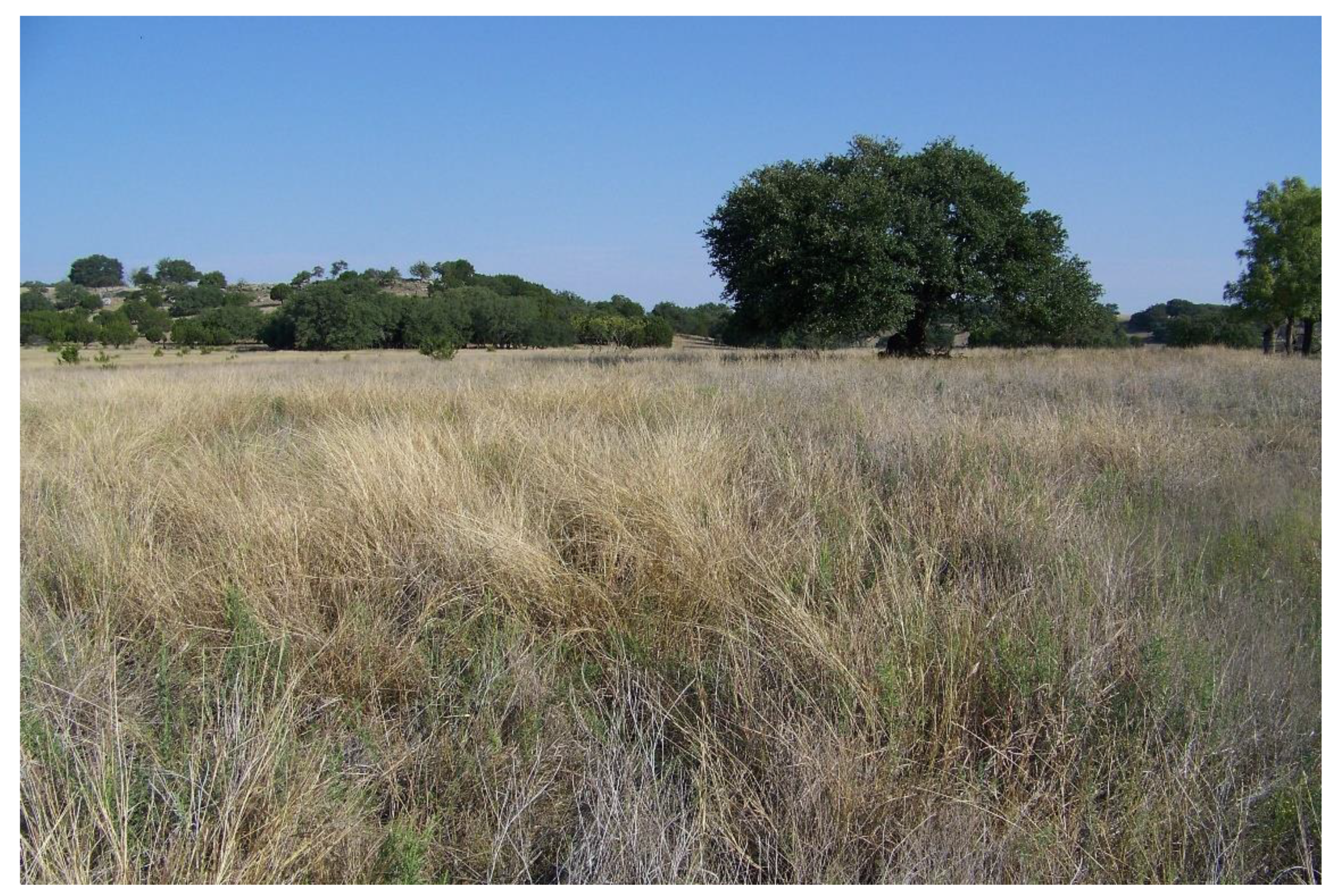
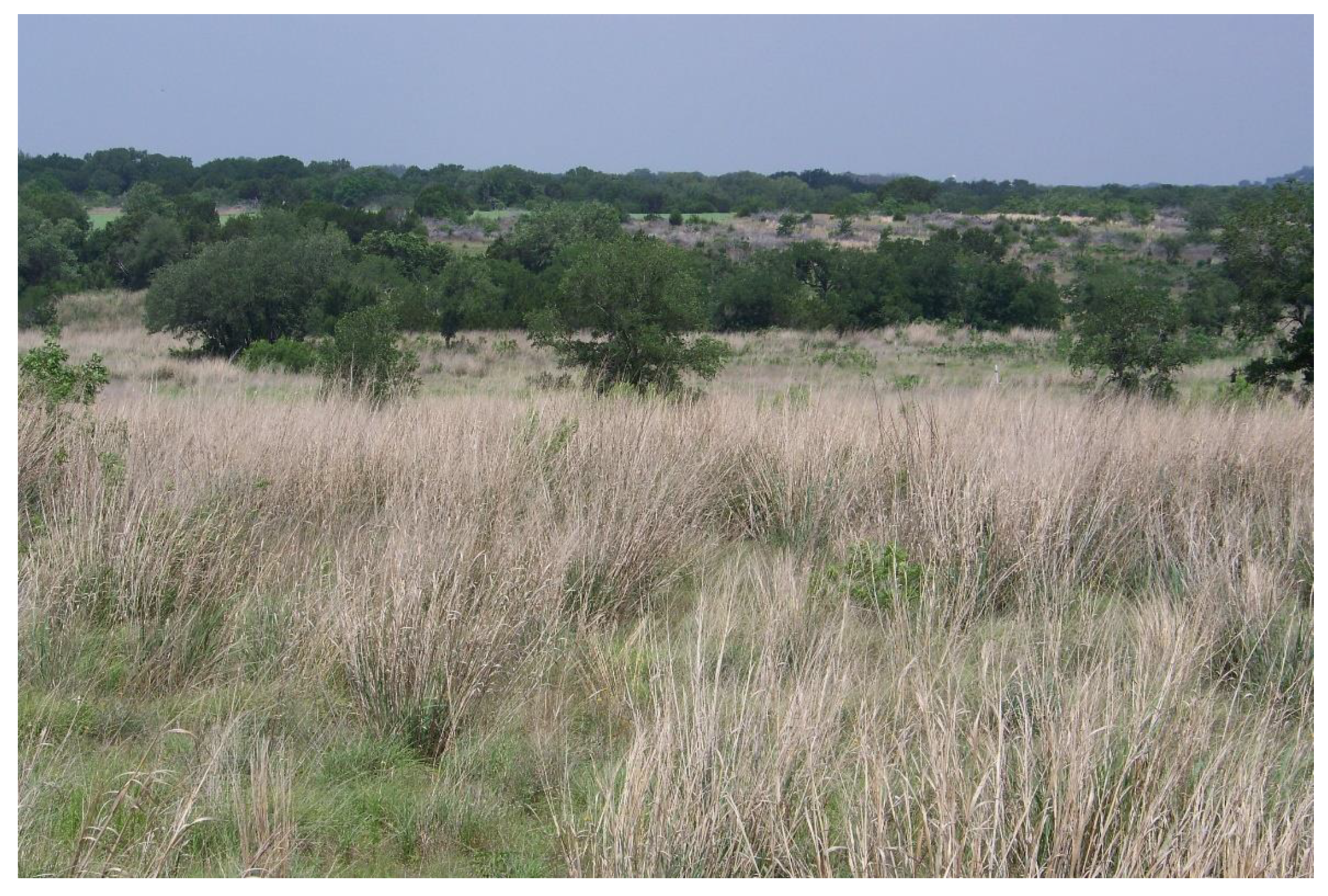
The study area is Coryell County, Texas (Figure 1) [38]. This county contains the Fort Hood Military Base, and within the county typical agricultural production includes cattle ranching, agronomy and pecan (Carya illinoinensis (Wangenh.) K. Koch) [38] production (Figure 2 and Figure 3). At one time, this region was part of the Republic of Mexico, then part of an independent country, the Republic of Texas, finally becoming annexed by the United States of America. The county is named after James Coryell (1803–1837), a Texan war hero [38]. In the county, the summers are hot (over 38 °C; 100 degrees F.) and the winters cool (minimum temperature is −12 °C; 10 degrees F.), but not cold (very little snowfall), averaging 32.5 inches (82.55 cm) of rain each year [38]. The growing season is typical over 260 days [38]. Guretzky et al. studied the interaction between grazing and the impact of military vehicle disturbance within the military base upon soil productivity [39]. Soils in the study area can be calcareous. Hatter and Morgan reported on the growth of three maple trees [Acer rubrum var. Drummondii (Hook. and Arn. Ex Nutt) Sarg., Acer saccharum Marsh. Subsp. saccharum, and Acer saccharum subsp. grandidentatum (Nutt. Desmarais)] in woody draws within the county [40]. Woody plants in the region include: Juniperus ashei J. Buchholz, Quercus fusiformis Small, and Quercus texana Buckley [38]. The mesic prairie is dominated by Schizachyrium scoparium (Michx.) Nash and Sorghastrum nutans (L.) Nash [41].

2.2. Statistical Analysis

The dependent variables are derived from vegetation yields in the county: wheat (Triticum aestivum L.) bushels per acre (one bushel is 0.363 hectoliters and one acre is 0.405 hectares, thus one bushel per acre is 0.1470 hectoliters per hectare), oats [Avena sativa L. (1753)] measured in bushels per acre, sorghum [Sorghum bicolor (L.) Moench] measured in bushels per acre, cotton lint (Gossypium hirsutum L.) measured in pounds per acre (one pound per acre is 0.18371 kg per hectare), Bermuda grass [Cynodon dactylon (L.) Pers.] in animal unit month (AUM), and rangeland production measured in pounds per acre. With principal component analysis (PCA), it is possible to examine how the measurements of seemingly disparate variables (such as weight or volume per area or animal unit months) can be examined as a group. This was the statistical problem that Kendall had a solution to [7]. The procedure standardizes each variable, allowing the variables to be equitably compared. If all vegetation types in the investigation do not covary in productivity, then the investigator must develop individually derived productivity equations. If they do covary, a universal plant productivity equation may be generated that is suitable for many types of crops. The PCA multivariate statistical approach is useful in both natural resource and social science studies, and has been applied in other types of studies including social/cultural science studies [3,4,41,42,43,44,45,46,47,48].
PCA facilitates the linear combination of productivity values to be combined through an equation to produce the dependent variable. With PCA, eigenvalues are produced (independent orthogonal dimensions). Typically, eigenvalues greater than 1.0 are considered to have the best potential for equation development. After the dependent variables are calculated through PCA, the independent soil variables, including main effects, squared terms and first order interaction terms, are applied in a regression study to determine the statistically best equation, that explains the largest variance while maintaining the set of regressors in the equation with a p-value equal to or less than 0.05. In this study 25 soil profiles were used in the analysis.
Li, He and Burley state: “In summary the process to conduct the research consists of measuring the properties of soil profiles and growing crops on these profile for approximately 10 years. Then employing a 40/30/20/10 depth weighting formula for each soil variable on each soil (independent variables). Next, use PCA to derive weighted linear combinations of plant yields/growth (dependent variable) across the soil profiles. Main effects, squared terms, and first order interaction terms are regressed to predict plant growth (Appendix A). The best predictor equations are those that explain the most variance without being over-specific, containing only significant variables (p ≤ 0.05).” [25]. The weighting formula examines four layers of the soil profile in increments of 30.48 cm to a depth of 1.2192 m. The average value for each variable within a specified layer is employed in the weighting formula.”

3. Results

Table 1 presents the six eigenvalues from the principal component analysis. The first eigenvalue contains 82.9% of the variance, and is the only eigenvalue greater than 1.0. Table 2 presents the eigenvector for each eigenvalue. In the first principal component, the eigenvector coefficients are all positive, and range from 0.3392 to 0.4262. This means it may be possible to construct a “six-crop” vegetation prediction model. Principal component number 2 suggests a range production model; however, the eigenvalue is below 1.0, indicating a meaningful model is unlikely. The third principal component has a strong cotton lint coefficient, with a value of 0.6826, suggesting an affiliation with a cotton lint model, but again the eigenvalue is below 1.0. For any model, productivity scores are without a unit of measure. Values below −2 indicate low productivity, and values above 2 indicate good productivity.
In the regression analysis, Table 3 presents the best equation derived from the first principal component. The soil factors of water holding capacity, electrical conductivity and topographic position are present in the equation. The table suggests that in the study area, water and less salty soils are important determinants. The regression explained 95.63% of the variance, with an overall significance value of p < 0.0001. Equation (1) represents the model derived from the regression results.
VP = −11.15 +(3.24 × SL) + (103.63 × AW) + (−0.19 × (SL**2)) + (−0.13 × SL × HC) + (−25.52 × SL × AW) + (−12.20 × AW × OM) + (1.54 × EC × OM)
where:
  • VP = vegetation productivity of the soil
  • SL = percent slope
  • AW = available water holding capacity
  • HC = hydraulic conductivity
  • OM = percent organic matter
  • EC = electrical conductivity

4. Discussion

To assess the validity of the model, the predicted soil productivity values of three soils were computed and examined: Topsey Soil Series C, Crawford Soil Series B and Eckrant Soil Series B [38]. Topsey soil is a deep loamy soil residing in uplands, which forms in calcareous sediment with slopes ranging from 3% to 8%. The soil is moderately suited for cropland. It contains layers of marl and shale beneath the soil. Crawford soil is composed of silty clay on uplands. The characteristics of the soil vary, depending upon when it is very wet or extremely dry. It must be carefully managed, but is suitable for cropland. At deeper depths in the soil profile, one encounters fractured limestone. Eckrant soil is a shallow, cobbly clay overriding limestone. The soil is mainly used as rangeland and not suitable for crops. The Crawford soil from the three soils is considered the most suitable for crops, and the Eckrant soil the least suitable. When Equation (1) is applied to these soils, the Tosey soil scores 0.04. The Crawford soil scores 1.32, and the Eckrant soil scores −3.15. The scores reflect the expected relative productivity between the three soils. In other words, the equation [Equation (1)], approximates expected general productivity.
The soil can be employed as a guide in the reconstruction of disturbed soil, such as that along highways, military ranges and urban areas. The equation is a quick assessment of performance, as all of the variables can be measured within a day. The most time-consuming variable to measure is the percent organic matter, which involves drying and burning the organic matter away. Available water holding capacity is often a matter of managing the soil structure and the amount of organic matter in the soil. The relatively quick assessment of a soil’s performance can be gleaned from the equation. Without the equation, it may take several years of crop production to assess a disturbed soil’s productivity. Thus, the equation can save time. The equation is not the final authority or arbitrator concerning vegetation productivity, but it is a tool for gaining insight into the general productivity of a soil in the county, especially for disturbed soils where the productivity may be unknown. The key features of the equation suggest that, for Coryell County, it is important to consider that:
  • Modest slopes assist productivity;
  • Maximizing available water hold capacity is beneficial;
  • Quick internal drainage (hydraulic conductivity) of slopes is not beneficial;
  • Organic matter in the soil increases productivity unless the available water holding capacity is already high;
  • Increased organic matter tempers soil electric conductivity (salty soils).
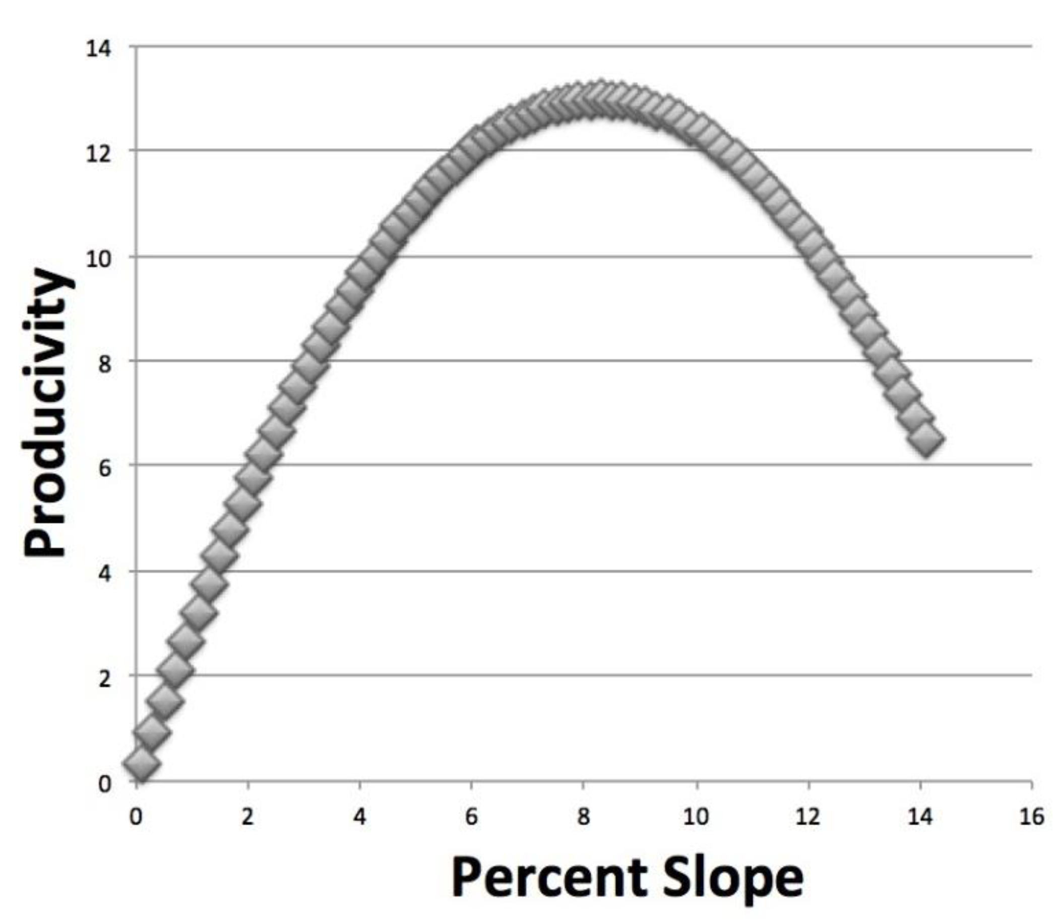
The equation is consistent with many other reported equations containing main effect terms, square terms and interaction terms [11,12,13,14,15,16,17,18,19,23,24,25]. The variable percent slope appears to be a curvilinear responding variable (Figure 4). The equation suggests that flat slopes are not preferred. As the slope increases the productivity increases, until the square term for slope overtakes the main effects term for slope, and causes the productivity score to decrease. The relationship does not imply the optimum slope, as slope is also an interaction term with hydraulic conductivity and available water holding capacity. In addition, the model does not imply that the other variables employed in the study (but not in the equation) are insignificant predictors, but rather that the variables in Equation (1) represent the combination with the most predictive power from the group of variables studied.
The value of this type of equation-building could be increased if productivity values for woody plants were added to the database, as this would be more useful for disturbed urban areas. Since pecans are grown in the county, it would have been helpful to have pecan productivity data to add to a modeling study. The study area has a limited number of soils to study. Often, counties that contain more soils for modeling, such as 50 to 60 soils, yield more reliable results. Still, an all-crop model was possible to build. Specific models for the second (specific rangeland model) and third (a cotton lint model) principal components may require more observations sets. When constructing a rangeland model, the amount of variance explained was low. When the cotton lint model was exposed to application of the cotton lint equation, the results did not co-vary with measured results, rendering the model nonsensical.
The relationship of these models to sustainability issues is especially pertinent when one examines landscape disturbance. As the planet’s population increases, much of the landscape is converted from native soils to highly disturbed and reconstructed soils. County soil surveys describing only native soils will become less useful, and new methods of soil description and assessment may be necessary. In Coryell County, Texas, the installation of an armed services testing range is an example. This is a land-use disturbance that is different to mining, and illustrates the breadth and diversity of landscape disturbances. The equation reported in this study can be applied to study the post-disturbance productivity of the soil, and aid in suggesting the properties that require modification in order to increase and maintain post-disturbance productivity.
As more of the planet’s landscape becomes disturbed by human activity, new measures to assess soil productivity may be required for the landscape fabric of urban savanna and emerging landscape urbanism [49]. Relatively little of the sustainability literature is focused on the soil, it being more focused upon buildings, business economics, supporting human cultures, protecting wildlife, air and water, and maintaining the integrity of native environments. The rise of sustainability as a scholarly topic may suggest a new direction for neo-soil productivity model applications and soil assessment, and give new life to a topic that has been relatively under-studied, despite a long history dating back to at least M. Kendall in 1939 [7].
The equation reported in this study will be added to the results from other reported models. Eventually, a model that considers location in the eastern 3/5ths of the United States (from Texas to Montana, to Maine and down to Florida) may be possible to construct, presenting a universal model to predict plant productivity for disturbed and reconstructed soils. Investigators around the world are encouraged to initiate and develop neo-soil metrics for their part of the world, in order to create a sustainable environment. There is an abundance of opportunities around the world in this general area of research. In 1864, George Perkins Marsh wrote about managing soil resources and the downfall of ancient civilizations [50]. As more land across the planet is being disturbed, managing these resources for sustainable purposes is just as relevant today. Being able to predict and guide the soil productivity of these disturbed soils is a contributor to, and possibly a foundation of, sustainable solutions and success at the most fundamental level. In the future, as native soils disappear, the authors of this study could imagine a forthcoming time where soil science and soil testing firms and experts would be employed to evaluate non-native, highly disturbed soils by measuring the soil profiles metrically, applying an equation, and producing a productivity number for a broad palette of vegetation types. While large portions of the landscape may no longer contain native soils, predicting, managing and maintaining soil productivity will remain important steps in creating a sustainable environment. New/evolving methods may be necessary to predict soil productivity.

Author Contributions

B.W. coded the data and ran the statistical analysis. J.B.B. supervised the research and prepared the manuscript. All authors have read and agreed to the published version of the manuscript.

Funding

This research was funded by the overseas visiting scholars of China Scholarship Council (No.201608430214).

Acknowledgments

The authors wish to thank Gerald Colter from the NRCS, Gatesville, Texas for supplying the images of the county.

Conflicts of Interest

The authors declare no conflict of interest.

Appendix A

Table A1. This is a table of the soil variables and their descriptive statistics.
VariableMeanStandard DeviationMinimumMaximum
% Clay24.2010.013.3052.23
Bulk Density1.380.071.231.56
% Organic Matter0.960.380.422.20
Available Water Holding0.150.030.040.19
% Rock Fragments0.521.130.008.00
Hydraulic Conductivity2.263.080.0417.87
Soil Reaction7.930.297.378.74
Electrical Conductivity1.811.900.009.18
% Slope3.283.571.0024.50
Topographic Position1.170.590.504.00

References

  1. Burley, J.B. Vegetation productivity equation compatibility with selected state environmental reclamation laws and regulations. In International Land Reclamation and Mine Drainage Conference and the Third International Conference on the Abatement of Acidic Drainage: Volume 4 of 4: Abandoned Mined Lands and Topical Issues; Bureau of Mines Special Publication SP 06D-94; United States Department of the Interior: Pittsburgh, PA, USA, 1994; pp. 294–303. [Google Scholar]
  2. Burley, J.B. Vegetation productivity equations: An overview. In Proceedings of the 1992 National Symposium on Prime Farmland Reclamation; Dunker, R.E., Barnhisel, R.I., Darmody, R.G., Eds.; Department of Agronomy, University of Illinois: Urbana, IL, USA, 1992; pp. 259–265. [Google Scholar]
  3. Burley, J.B.; Thomsen, C.H. Multivariate techniques to develop vegetation productivity models for neo-sols. In Proceedings of the 1987 Symposium on Surface Mining, Hydrology, Sedimentology and Reclamation; University of Kentucky: Lexington, KY, USA, 1987; pp. 153–161. [Google Scholar]
  4. Burley, J.B. Methodology for building soil based vegetation productivity equations: A statistical approach. In Proceedings of the Thirteenth Annual Meeting American Society for Surface Mining and Reclamation: Successes and Failures: Applying Research Results to Insure Reclamation Success, Knoxville, TN, USA, 18–23 May 1996; Daniels, W.L., Burger, J., Zipper, C.E., Eds.; Virginia Tech Research Division, Powell River Project: Blacksburg, VA, USA, 1996; pp. 789–798. [Google Scholar]
  5. Roecher, S.; Thomas, P.; Beaudette, D.; Willis, K. Looking Back: The History of Soil Survey Thru Metrics; North Central Cooperative Soil Survey Workshop: Brookings, SD, USA, 2018. Available online: https://www.researchgate.net/publication/328890443_Looking_Back_The_History_of_Soil_Survey_Thru_Metrics (accessed on 2 June 2020).
  6. Soil Survey Division Staff; United States Department of Agriculture. Soil Survey Manual. United States; Handbook No. 18; Department of Agriculture: Washington, DC, USA, 1993.
  7. Kendall, M.G. The Geographical Distribution of Crop Productivity in England. J. R. Stat. Soc. 1939, 102, 21–48. [Google Scholar] [CrossRef]
  8. Jeanne, T.; Parent, S.-É.; Hogue, R. Using a soil bacterial species balance index to estimate potato crop productivity. PLoS ONE 2019, 14, e0214089. [Google Scholar] [CrossRef]
  9. Zak, J.; Willig, M.; Moorhead, D.; Wildman, H. Functional diversity of microbial communities: A quantitative approach. Soil Boil. Biochem. 1994, 26, 1101–1108. [Google Scholar] [CrossRef]
  10. Natural Resource Conservation Service. Annual Data Refresh of Soil Survey Data; United States Department of Agriculture, Natural Resource Conservation Service: Washington, DC, USA, 2018. Available online: http://nrcs.usda.gov (accessed on 2 June 2020).
  11. Burley, J.B.; Thomsen, C.H.; Kenkel, K. Development of an agricultural productivity model to reclaim surface mines in Clay County, Minnesota. Environ. Manag. 1989, 13, 63–638. [Google Scholar]
  12. Burley, J.; Thomsen, C.H. Application of an agricultural soil productivity equation for reclaiming surface mines: Clay County, Minnesota. Int. J. Surf. Min. Reclam. Environ. 1990, 4, 139–144. [Google Scholar] [CrossRef]
  13. Burley, J.B. A vegetation productivity equation for reclaiming surface mines in Clay County, Minnesota. Int. J. Surf. Min. Reclam. Environ. 1991, 5, 1–6. [Google Scholar] [CrossRef]
  14. Burley, J.B. Sugarbeet Productivity Model for Clay County Minnesota. J. Sugarbeet Res. 1990, 27, 50–59. [Google Scholar] [CrossRef]
  15. Burley, J.B.; Bauer, A. Neo-sol Vegetation Productivity Equations for Reclaiming Disturbed Landscapes: Central Florida Example. J. Am. Soc. Min. Reclam. 1993, 1993, 334–347. [Google Scholar] [CrossRef]
  16. Burley, J.B. A multi-county vegetation productivity equation for soil reclamation. In Proceedings of Sudbury’95-Mining and the Environment; Hynes, T.P., Blanchette, M.C., Eds.; CANMET: Ottawa, ON, Canada, 1995; Volume 3, pp. 1113–1122. [Google Scholar]
  17. Burley, J.B.; Polakowski, K.J.; Fowler, G. Constructing vegetation productivity equations by employing undisturbed soils data: An Oliver County, North Dakota case study. In Proceedings of the Thirteenth Annual Meeting American Society for Surface Mining and Reclamation: Successes and Failures: Applying Research Results to Insure Reclamation Success, Knoxville, TN, USA, 18–23 May 1996; Daniels, W.L., Burger, J., Zipper, C.E., Eds.; Virginia Tech Research Division, Powell River Project: Blacksburg, VA, USA, 1996; pp. 393–401. [Google Scholar]
  18. Burley, J.B.; Fowler, G.W.; Polakowski, K.; Brown, T.J. Soil Based Vegetation Productivity Model for the North Dakota Coal Mining Region. Int. J. Surf. Min. Reclam. Environ. 2001, 15, 213–234. [Google Scholar] [CrossRef]
  19. Burley, J. A spatial application of a vegetation productivity equation for neo-sol reconstruction. J. Am. Soc. Min. Reclam. 1999, 1999, 708–714. [Google Scholar] [CrossRef]
  20. Burley, J.B.; Gray, D. Soil ordination: Implications for post-mining disturbance land-uses. J. Am. Soc. Min. Reclam. 2001, 2001, 241–245. [Google Scholar] [CrossRef]
  21. Burley, J.B. Environmental Design for Reclaiming Surface Mines; Edwin Mellen Press: Lewiston, NY, USA, 2001. [Google Scholar]
  22. Le Cleac’h, G.; Salles, G.M.; Burley, J.B. Vegetation productivity model for Grand Traverse County. In Michigan. 21st National Meeting of the American Society of Mining and Reclamation and The 25th West Virginia Surface Mine Drainage Task Force. Morgantown, WV, USA, 18–24 April 2004; ASMR: Lexington, KY, USA, 2004; pp. 1176–1191. [Google Scholar]
  23. Chang, Q.; Bai, Y.; Burley, J.B.; Partin, S. Soil-based vegetation productivity model for mined lands in Chippewa County, Wisconsin. In Recent Advances in Environment, ecosystems and Development, Proceedings of the 13th International Conference on Environment, Ecosystems and Development (EED’15), Kuala Lumpur, Malaysia, 23–25 April 2015; Bulucea, A., Ed.; Energy, Environmental and Structural Engineering Series|35; World Scientific and Engineering Academy and Society: Athens, Greece, 2015; pp. 15–22. [Google Scholar]
  24. Bai, Y.; Chang, Q.; Guo, C.; Burley, J.B.; Partin, S. Neo-sol productivity models for disturbed lands in Wisconsin and Georgia, USA. Int. J. Energy Environ. 2016, 10, 52–60. [Google Scholar]
  25. Burley, J.B.; Wu, Z.; He, S.; Li, X. Soil-based vegetation productivity models for disturbed lands along the north and central western Great Plains, USA. J. Adv. Agric. Technol. 2020. in publication. [Google Scholar]
  26. Burley, J.B.; Machemer, T. From Eye to Heart: Exterior Spaces Explored and Explained; Cognella Academic Publishing: San Diego, CA, USA, 2016. [Google Scholar]
  27. Humphries, R.N.; Thompson, R.J.K.; Heames, M.D. Case study: Appraisal of four soil-based metrics in the establishment of sustainable upland grassland at a mine site in south wales, united kingdom. J. Am. Soc. Min. Reclam. 2019, 2019, 1–21. [Google Scholar] [CrossRef]
  28. Burley, J.B.; Li, X.; He, S. Metrics Evaluating Multivariate Design Alternatives: Application of the Friedman’s Two-way Analysis of Variance by Ranks: A Personal Reflection; Whitemud Academics: Perrinton, MI, USA, 2020; p. 36. [Google Scholar]
  29. Burley, J.B.; Li, N.; Ying, J.; Tian, H.; Troost, S. Chapter 3: Metrics in master planning low impact development for Grand Rapids, Michigan. In Sustainable Urbanization; Egren, M., Ed.; Intech: Rijeka, Croatia, 2016; pp. 61–86. [Google Scholar]
  30. Duan, X.-W.; Han, X.; Hu, J.-M.; Feng, D.-T.; Rong, L. A novel model to assess soil productivity in the dry-hot valleys of China. J. Mt. Sci. 2017, 14, 705–715. [Google Scholar] [CrossRef]
  31. Rodrique, J.A.; Burger, J.A. Forest soil productivity of mined land in the midwestern and eastern coalfield regions. Soil Sci. Soc. Am. J. 2004, 68, 833–844. [Google Scholar] [CrossRef]
  32. Barnhisel, R.I.; Hower, J.M. The use of productivity index to predict corn yields of restored prime farmland. In International Land Reclamation and Mine Drainage Conference and the Third International Conference on the Abatement of Acidic Drainage: Volume 3 of 4: Vegetation and Reclamation; Bureau of Mines Special Publication SP 06D-94; United States Department of the Interior: Pittsburgh, PA, USA, 1994; pp. 20–27. [Google Scholar]
  33. Peng, L.; Zhanbin, L.; Zhang, Z. An index system and method for soil productivity evaluation on the hillsides on the Loess Plateau. In 12th ISCO Conference; Tsinghua University Press: Beijing, China, 2002. [Google Scholar]
  34. Dyson, F. Disturbing the Universe; Basic Books; Sloan Foundation Science Series Edition: New York, NY USA, 1981. [Google Scholar]
  35. Burras, C.L.; Miller, G.A.; Fenton, T.E.; Sassman, A.M. Corn Suitability Rating 2 (CSR2) Equation and Component Values; Iowa State University: Ames, IA, USA, 2015. [Google Scholar]
  36. Schaetzl, R.J.; Krist, F.J., Jr.; Miller, B.A. A taxonomically based ordinal estimate of soil productivity for landscape-scale analysis. Soil Sci. 2012, 177, 28–299. [Google Scholar] [CrossRef] [Green Version]
  37. Voltr, V. Concept of soil fertility and soil productivity: Evaluation of agricultural sites in the Czech Republic. Arch. Agron. Soil Sci. 2012, 58, S243–S251. [Google Scholar] [CrossRef]
  38. McCaleb, N. Soil Survey of Coryell County, Texas; United States Department of Agriculture, Soil Conservation Service: Washington, DC, USA, 1985.
  39. Guretzky, J.A.; Anderson, A.B.; Fehmi, J.S. Grazing and Military Vehicle Effects on Grassland Soils and Vegetation. Gt. Plains Res. J. Nat. Soc. Sci. 2006, 16, 51–61. [Google Scholar]
  40. Hatter, M.D.; Morgan, D.L. Growth and visual responses of three Southwestern Acer taxa to high-salt irrigation water. J. Environ. Hortic. 1992, 10, 118–120. [Google Scholar]
  41. Anderson, A.B.; Wang, G.; Fang, S.; Gertner, G.Z.; Güneralp, B.; Jones, D. Assessing and predicting changes in vegetation cover associated with military land use activities using field monitoring data at Fort Hood, Texas. J. Terramech. 2005, 42, 207–229. [Google Scholar] [CrossRef]
  42. Burley, J.B. Constructing Interpretable Environments from Multidimensional Data: GIS Suitability Overlays and Principal Component Analysis. J. Environ. Plan. Manag. 1995, 38, 537–550. [Google Scholar] [CrossRef]
  43. Burley, J.B.; Singhal, V.B.P.; Burley, C.J.; Fasser, D.; Churchward, C.; Hellekson, D.; Raharizafy, I. Citation Analysis of Transportation Research Literature: A Multi-Dimensional Map of the Roadside Universe. Landsc. Res. 2009, 34, 481–495. [Google Scholar] [CrossRef]
  44. Gellar, D.; Bauer, A.; Burley, J.B. Mapping the reclamation regulation universe in the United States and Canada: A 1994/95 topology experience. In Sudbury’99 Mining and the Environment II: An Integrated Approach to Planning and Rehabilitation for the Future, Sudbury, ON, Canada, 13–17 September 1999; Goldsack, D., Belizile, N., Yearwood, P., Hall, G., Eds.; Laurentian University: Sudbury, ON, Canada, 1999; Volume 3, pp. 991–1000. [Google Scholar]
  45. Qi, J.; Wang, S.; Burley, J.B.; Machemer, T. Defining ecological regions in Michigan based on native tree distributions. Landsc. Archit. 2012, 6, 138–145, (translated by Wang, S.). [Google Scholar]
  46. Xu, Y.; Burley, J.B.; Machemer, R.; Allen, A. A dimensional comparison between classical Chinese gardens and modern Chinese gardens. WSEAS Trans. Environ. Dev. 2016, 12, 200–213. [Google Scholar]
  47. Xu, H.; Burley, J.B.; Crawford, P.; Schutzki, R. Cross-cultural ordination of burial sites. Int. J. Cult. Herit. 2017, 2, 92–104. [Google Scholar]
  48. Xu, H.; Burley, J.B.; Crawford, P.; Wang, Y.; Yue, Z.; Schutzki, R. An ordination of western and Chinese burial sites. WSEAS Trans. Environ. Dev. 2017, 13, 452–469. [Google Scholar]
  49. Burley, J.B. The Emergence of Landscape Urbanism: A Chronological Criticism Essay. Land 2018, 7, 147. [Google Scholar] [CrossRef] [Green Version]
  50. Marsh, G.P. Man and Nature: Physical Geography as Modified by Human Action; Scribner, C.: New York, NY, USA, 1864. [Google Scholar]
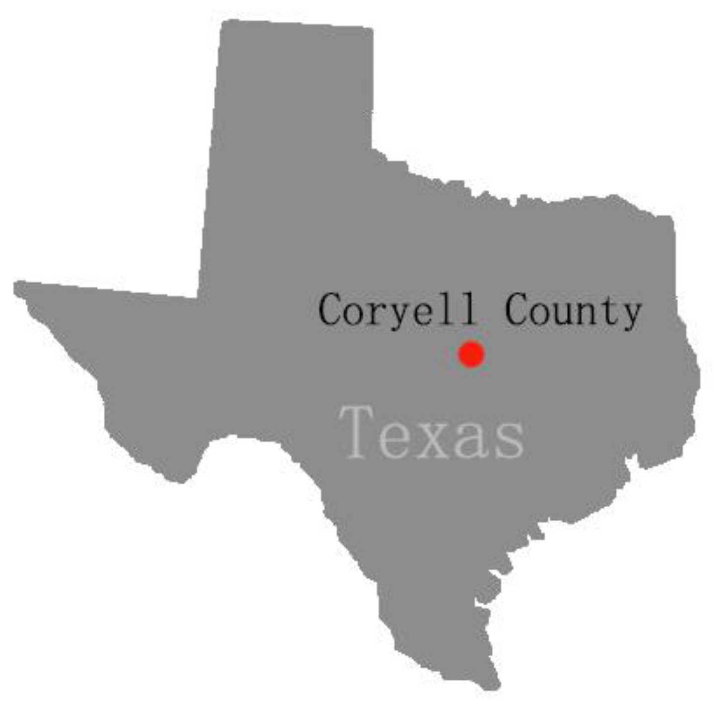
Figure 1. A map illustrating the general location of Coryell County in the State of Texas.
Sustainability 12 05240 g001
Figure 2. A photograph of the rangeland in Coryell County in the State of Texas; notice the rock outcrop in the distant background left (courtesy of Texas NRCS).
Sustainability 12 05240 g002
Figure 3. Another image of the rolling rangeland landscape in Coryell County in the State of Texas (courtesy of the Texas NRCS).
Sustainability 12 05240 g003
Figure 4. A plot of the curvilinear relationship of slope to soil productivity with the equation: Productivity = (3.24 × Slope) + (−0.19 × Slope × Slope).
Sustainability 12 05240 g004
Table 1. This table presents the eigenvalues from the crop variables.
Eigenvalues of the Covariance Matrix
Principal ComponentEigenvalueDifferenceProportionCumulative
14.973866624.589078690.82900.8290
20.384787930.088667570.06410.8931
30.296120370.098897050.04940.9425
40.197223320.088730280.03290.9753
50.108493040.068984320.01810.9934
60.03950872 0.00661.0000
Table 2. This table presents the eigenvector coefficients for each crop across each principal component.
Eigenvectors
Prin1Prin2Prin3Prin4Prin5Prin6
WHEAT0.403243−0.051705−0.706695−0.2618110.5143480.046954
OATS0.430054−0.119093−0.137170−0.193362−0.6840430.526072
GRAIN SORGHUM0.436191−0.1889800.045913−0.135658−0.292321−0.817351
COTTON LINT0.401516−0.2146180.682568−0.3369500.4106640.211291
BERMUDAGRASS0.407866−0.2369530.0180090.8695260.1157540.087745
POTENTIAL ANNUAL PRODUCTION0.3669020.9193600.1159070.0777930.005929−0.025284
Table 3. This table presents the regression results from the best model for the first principal component.
VariableParameter EstimateStandard ErrorType II SSF ValuePr > F
Intercept−11.151.7612.2839.98< 0.0001
SL3.240.084.9416.100.0009
AW103.6311.1226.6686.83< 0.0001
SL2−0.190.043.3010.740.0044
SLHC−0.130.052.367.700.0130
SLAW−25.524.2311.1836.41< 0.0001
AWOM−12.202.795.8819.140.0004
ECOM1.540.434.0013.030.0022