Vibration-Based Seismic Damage States Evaluation for Regional Concrete Beam Bridges Using Random Forest Method

Abstract

Transportation networks play an important role in urban areas, and bridges are the most vulnerable structures to earthquakes. The seismic damage evaluation of bridges provides an effective tool to assess the potential damage, and guides the post-earthquake recovery operations. With the help of structural health monitoring (SHM) techniques, the structural condition could be accurately evaluated through continuous monitoring of structural responses, and evaluating vibration-based features, which could reflect the deterioration of materials and boundary conditions, and are extensively used to reflect the structural conditions. This study proposes a vibration-based seismic damage state evaluation method for regional bridges. The proposed method contains the measured structural dynamic parameters and bridge configuration parameters. In addition, several intensity measures are also included in the model, to represent the different characteristics and the regional diversity of ground motions. The prediction models are trained with a random forest algorithm, and their confusion matrices and receiver operation curves reveal a good prediction performance, with over 90% accuracy. The significant parameter identification of bridge systems and components reveals the critical parameters for seismic design, disaster prevention and structure retrofit.

1. Introduction

Earthquakes are a major natural hazard that impact urban sustainable development and infrastructure safety [1]. Bridges are the most vulnerable elements in the urban transportation system. The damage state evaluation of regional bridges informs bridge managers about the possible damages and risks in a seismic event [2,3,4]. Due to traffic loads and environmental effects, seismic demand and the capacity of in-service bridges are different from the original conditions [5,6]. To make an informed decision regarding pre-earthquake maintenance and post-earthquake recovery, it is critical to evaluate the seismic damage states of bridges based on their real-time conditions.

With the development of structural health monitoring, quite a few structural health monitoring systems (SHMS) are installed on infrastructures to record the long-term behaviors [7,8]. Information obtained from SHMS is mostly used to assess the long-term deterioration process due to physical aging and traffic loads, while there are still some limitations in identifying the location and degree of structural damages under the earthquake: (1) nonlinear system identification: ground motions lead to structural nonlinear failure, and existing techniques are not easily able to identify strong nonlinear behaviors; (2) distributed damage: multiple local damages appear in a large number of components after the earthquake; (3) signal interruption: signal cables and electric cables might be cut off in the earthquake, which obstructs engineers from obtaining the in-earthquake and post-earthquake data. In view of the limitations of seismic monitoring, it would be appropriate to update the structural conditions with SHMS before the earthquake.

Data-driven methods are approaches that apply machine learning algorithms to directly use the measured data as input to evaluate the structural conditions. Sajedi and Liang [9] developed a method to diagnose structural real-time damages using the support vector machine (SVM). It precisely predicted the existence, location and severity of damages. Clustering methods [10] and neural networks [11] were used for condition assessments and damage detections. Jang and Smyth [12] explored the three most popular machine learning models to describe the relationship between environmental effects and modal properties, where random forests (RF) obtained higher efficiency with the same prediction accuracy. Since data-driven models directly identify the data features of structural condition changes, they do not need any prior knowledge.

Vibration-based structural condition assessment is a conventional and effective approach to detecting structural damages only using structural mechanism characteristics [13,14,15], such as natural frequencies, modal damping, curvature mode shapes, etc. Based on the first three natural frequencies, Morassi and Rollo [16] developed a method for assessing the condition of a simply supported beam under flexural vibrations. Lin and Cheng [17] presented a technique with curvature mode shapes to detect the damages of a free–free beam. Kbiem and Lien [18] derived frequency change indicators and used them to determine the structural condition and detect the locations of cracks. The availability of vibration-based structural condition assessments provides a unique opportunity to evaluate seismic damage states based on updated structural conditions.

Previous studies used comprehensive geometrical and material parameters to reflect the real performance of each component [19,20]. Material stiffnesses and boundary conditions affect the structural seismic performance, but their correct determination is labor-consuming. Abutments provide a great source of energy dissipation and decrease the probability of the unseating of the bridge beams [21]. Shear keys assist in constraining the relative lateral displacement between the beam and the abutments, and two adjacent beam segments [22]. Bearings transfer the horizontal friction forces between superstructures and substructures. Bridge foundations transfer structural loads to the underlying soil. The bridge column is one of the main components in resisting the earthquake, and its seismic performance depends on the area of reinforcement, the strength of core concrete, and built-in reinforcement. Although these detailed material stiffness and boundary condition parameters make a great contribution to enhancing the model’s accuracy, it is labor-consuming to get these real values. Since the structural dynamic characteristics can reflect the material and boundary conditions, it is convenient for the monitored bridges to use the measured structural dynamic parameters to represent their real-time seismic performances.

Earthquake excitations of each bridge are diversified across regional scales [23,24]. Sensors installed on the bridges and the nearby seismographs record the time-history of the excreted ground motion, and detailed characteristics of ground motions could be easily extracted to reflect their intensities. In previous studies, most of the research selects only one intensity measure (IM) to represent the seismic hazard; peak ground acceleration (PGA) is the most commonly used. Padgett [25] suggested that the PGA is a suitable selection to represent the severity of the earthquake ground motion, due to its efficiency and ease-of-implementation. The relative efficiency of PGA with some other IMs [peak ground velocity (PGV), peak ground displacement (PGD) and spectral acceleration at 1 s] has been carried out. However, since a large PGA value does not always induce severe structural damage, other IM, such as PGV, PGD, the time duration of strong motion and spectrum intensity, should also be considered.

Seismic damage state evaluation is a kind of classification problem [26]. RF is an ensemble learning method, and it consists of bagging and random feature selection techniques to generate a large quantity of independent decision trees [27,28]. The trained model is more robust than a single decision tree, and less likely to overfit. Jia [29] used RF to train the model with the data of the Wenchuan earthquake and the Tangshan earthquake. The results showed a good performance for assessing the damage states of two bridges. Kiani [30] compared multiple classification algorithms for assessing the damage states of buildings. RF has the highest efficiency in predicting the structural seismic damages compared with other methods. RF can robustly handle high dimensional, large datasets with outliers and non-linear data. Its parallel computing can split the process into multiple machines to save computation time. Each decision tree has a high variance, but low bias. Since RF averages the variances of all the trees, we could get a low bias and moderate variance model, even for an unbalanced dataset [31].

This paper proposes a vibration-based damage state evaluation method for concrete beam bridges using the RF method. The models contain bridge design parameters, structural dynamic characteristics and ground motion parameters. Design parameters represent the bridge configuration. Instead of traditional structural material strength and boundary stiffness parameters, dynamic characteristics are included in the models to represent bridge real-time conditions. These structurally related parameters are easy to be obtained for a bridge installed with SHMS. As for ground motions, several parameters, related to the peak effect, spectral characteristics and time duration of strong motions, are included in the models. RF classification methods are used to predict the damage state. To verify the effectiveness of the proposed method, the prediction accuracy of the proposed models and traditional models are compared. Besides, the confusion matrix and receiver operating characteristic curves of the proposed models are illustrated to manifest their high efficiency. For each bridge component, the relative significant parameters are also identified.

2. Numerical Modeling Techniques

This study selects the short- and medium-span beam bridges to establish regional damage state evaluation models. The three-dimensional simplified numerical models are developed by the Open System for Earthquake Engineering Simulation Platform (OpenSEES), incorporating the nonlinear material and geometrical behaviors. A typical layout of the selected short- and medium-span beam bridge model employed in this study is illustrated in Figure 1.

In general, there are four common types of the superstructure for short- and medium-span beam bridges, that is, RC simply supported slab bridge, prestressed concrete simply supported hollow slab bridge, prestressed T-shaped concrete beam bridge, and prestressed box-shaped concrete beam bridge. The design references of short- and medium-span beam bridges in each country are relatively similar. Taking the design references in China as an example, the Ministry of Transport issued the standard drawings to guide the design of each type of bridge. The section dimensions, reinforcement layouts, reaction of superstructures, and other details for standard span length beam are given. This information can provide an efficient basis for the establishment of numerous standardized short- and medium-span beam bridges.

2.1. Model Establishment

The beam is modeled with the elastic beam-column element, since this would remain elastic during the earthquake. The mass of the superstructures acts as the inertial force for the whole bridge, so it is precisely calculated by the reaction of the superstructures. Due to the proposed model containing the dynamic characteristics, the stiffness of superstructures is also calculated with the given section’s dimensions. The transverse beam is modeled with the massless rigid link element to illustrate the torsion of the beam. Most of the short- and medium-span bridges are designed with laminated rubber bearings, and their stiffness impacts the bridge’s nonlinear response and dynamic characteristics. Bearing is assumed to be a perfectly elastic model [32], where its stiffness is determined by the bridge’s seismic design code [33]. Beam caps remain elastic during the earthquake, so its mass is modeled on the top of the columns. Columns are modeled with the fiber-based displacement beam-column element. In the fiber sections, the Steel02 material model with a hardening factor of 0.01 is used to simulate the reinforcement behavior. The Concrete01 and Concrete02 material models are used to account for the cover and core concrete behavior, respectively. Each bridge foundation is modeled with three translational linear springs and three rotational linear springs.

The influence of the abutment on the seismic damage of the bridge is significant; quite a few studies [21,34,35] have presented the intrinsic issues in abutment modeling. In this study, a complex series and parallel spring system account for the abutment’s dynamic behaviors, and these are all modeled with zero-length elements. In the longitudinal direction, the effects of elastomeric bearing, gap, abutment piles (active soil) and soil backfill material (passive soil) are considered. The gap is modeled with the pounding springs [36], which contain a gap and bilinear high stiffness. Before the gap closure, the force transmits from the beam to the bearings and gaps, and then to the abutment piles and backfill soils [37]. After the gap closure, the beam, along with the bearing systems, collide directly with the abutment, which initiates the full passive earth pressure. In the transverse direction, the effects of elastomeric bearing, concrete shear keys and abutment piles (active soil) are considered. The elastomeric bearing and shear keys act in parallel. This combined parallel system is in series with the abutment piles (active soil). According to Caltrans [38], the ultimate strength of the shear key is determined to be 30% of the superstructure dead load. A tri-linear hysteric backbone curve is defined for shear keys.

2.2. Model Verification

Accurate bridge dynamic models are an effective basis for the following seismic damage analysis. There are quite a few short- and medium-span bridges installed with SHMS [39]. Since the occurrence of earthquakes is extremely rare, it is quite hard to measure the seismic response. This paper compares the bridge dynamic characteristics between measured real bridges and the corresponding numerical models, to ensure the reliability of the proposed modeling techniques.

Nanli river bridge is located on the Xinglin Highway in Hebei province, China. It is a typical prestressed box-girder skew bridge with a span of 30 m. The bridge cross-section consists of four small box longitudinal beams, and there are three transversal beams at the quarter and middle of the span to link all these longitudinal beams. The layout of the monitored span and installed sensors is shown in Figure 2. Five sections are installed with different kinds of sensors, and static levels are used to measure the displacement of the bridge; thermometers can compensate the temperature error of the measured data; and dynamic characteristics can be identified from strain gauges and accelerometers.

Using the Stochastic Subspace Identification (SSI) method to analyze the response data of the accelerometers, the bridge frequencies can be accurately measured. Using the proposed numerical modeling techniques combined with real bridge parameters, the frequency of the numerical model can be extracted. Besides, the accuracies of mode shapes are calculated with the modal assurance criterion (MAC). The first three-order frequencies and MACs are compared in

Table 1. Frequency comparison of simulation result and measured result.

Order	Simulated Frequency (Hz)	Measured Frequency (Hz)	Error Percentage	MAC
1	4.573	4.636	−1.4%	0.992
2	5.486	5.482	0.073%	0.990
3	8.065	8.132	−0.83%	0.990

. It can be seen that the difference between these two sources is very small, indicating that the proposed numerical modeling techniques are reliable.

3. Uncertain Parameters

This paper proposes a seismic damage evaluation method for regional monitored concrete beam bridges. Unlike the traditional seismic damage evaluation method, the selected parameters in the proposed method are conveniently obtained for a monitored bridge. To ensure the high accuracy of the damage prediction, the traditional method employs the material stiffness and boundary condition parameters to simulate the real condition of bridges, however, the proposed method uses bridge real-time dynamic characteristics.

3.1. Material and Boundary Parameters for Traditional Unmonitored Bridges

In the traditional method, many bridge geometrical and material parameters are included, as listed in

Table 2. Structural Uncertainties.

Traditional Method		Proposed Method
Variables	Parameters	Variables	Parameters
$R_1$	Span	$P_1$	Span
$R_2$	Number of Spans	$P_2$	Number of Spans
$R_3$	Number of Beams	$P_3$	Column height
$R_4$	Column height	$P_4$	Diameter of Column
$R_5$	Diameter of Column	$P_5$	Number of Columns
$R_6$	Number of Columns	$P_6$	Skew angle
$R_7$	Skew angle	$P_7$	1st frequency
$R_8$	Longitudinal reinforcement ratio of column	$P_8$	2nd frequency
$R_9$	Concrete compressive strength of column	$P_9$	3rd frequency
$R_{10}$	Reinforcement yield strength of column	$P_{10}$	4th frequency
$R_{11}$	Rotational stiffness of foundation	$P_{11}$	5th frequency
$R_{12}$	Translational stiffness of foundation

. Geometrical parameters selected from the main design parameters illustrate the bridge configuration. Span ($R_1$) and Number of Spans ($R_2$) depict the longitudinal layout of bridges. Number of Beams ($R_3$) depicts the transversal layout of bridges. Since the proposed modeling technique is based on the aforementioned standard drawings, the mass and stiffness of the superstructures are easy to determine with these three parameters. Column height ($R_4$), Diameter of Column ($R_5$) and Number of Columns ($R_6$) are used to determine the layout of substructures. Bearing stiffness is determined with the mass of superstructures and seismic design codes. Skew angle ($R_7$) makes it possible to simulate the skew bridges.

Material parameters and boundary stiffness parameters are included to modify the bridge response. Since the column plays an important role in the earthquake event, longitudinal reinforcement ratio ($R_8$), concrete compressive strength ($R_9$) and reinforcement yield strength ($R_{10}$) are used to calibrate the real performance of the column. As for the foundation, rotational stiffness ($R_{11}$) and translational stiffness ($R_{12}$) are the key stiffness. Abutment pile stiffness and backfill stiffness are determined with the soil condition. These parameters ($R_8~R_{12}$) are determined with the original design values, so they can not reflect the real-time structural conditions.

This paper establishes 672,000 numerical models with these modeling parameters, to comprehensively consider all kinds of regional beam bridges. The Latin Hypercube Sampling (LHS) method [40] is a stratified sampling method for generating a near-random sample of parameter values from a multidimensional distribution. To perform the stratified sampling, the cumulative probability is divided into segments. It randomly selects samples from each segment using a uniform distribution, and then maps to the correct representative value the variable’s actual distribution. Once each variable has been sampled using this method, a random grouping of variables is selected with the independent uniform selection. LHS aims to spread the sample points more evenly across all possible values. In this paper, the samples of the numerical three-dimensional bridge model are generated by sampling across a certain range of uncertain parameters using the LHS method.

3.2. Dynamic Characteristic Parameters for Proposed Monitored Bridges

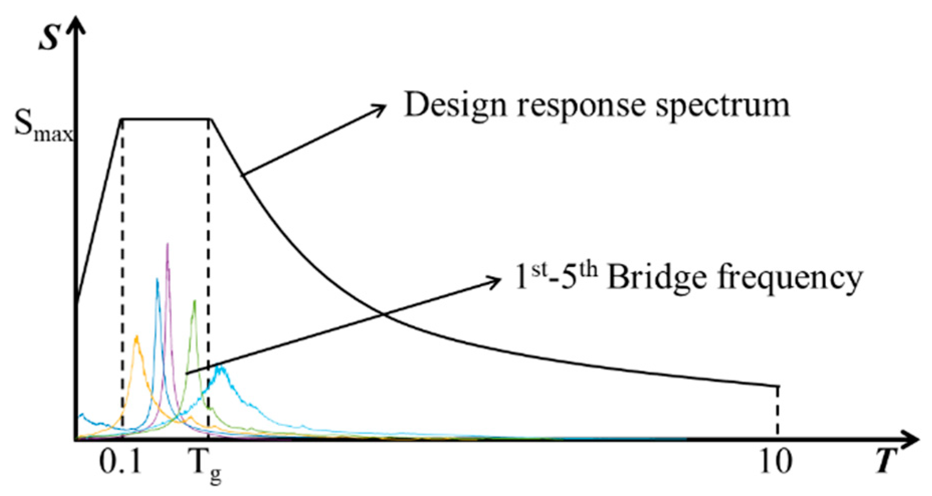
In the proposed method, the bridge dynamic characteristics parameters are included to replace some material and stiffness parameters. Since the bridge geometrical parameters ($P_1$~$P_6$) are easy to obtain from the design documents or technical reports, they are preserved in the model to illustrate the bridge configuration. Bridge dynamic characteristics are important indicators of the bridge condition, as their fluctuations could reflect the deterioration of the material and stiffness performances. According to the seismic design code, the maximum acceleration response spectrum appears between 0.1 s and the characteristic period ($T_g$). This interval generally contains the first five orders of bridge frequencies ($P_7$~$P_{11}$), as illustrated in Figure 3. With the help of modern signal processing techniques, frequencies ($P_7$~$P_{11}$) of the monitored bridge can be identified. These parameters mainly aim to represent the real-time condition of the measured bridges. Although the dynamic characteristic parameters might be influenced by the bridge design parameters, these parameters can be used together to effectively determine the configurations and real-time conditions of the measured bridges. The proposed method uses theses 11 parameters (Table 2) to predict seismic damage states for regional monitored beam bridges.

Generally, the proposed dynamic characteristic parameters can be measured either before or after the earthquake. If they are measured before the earthquake, this could have implications on the post-earthquake emergency traffic and recovery operations; If they are measured after the earthquake, the post-earthquake damage states could be identified without much delay.

3.3. Intensity Measures

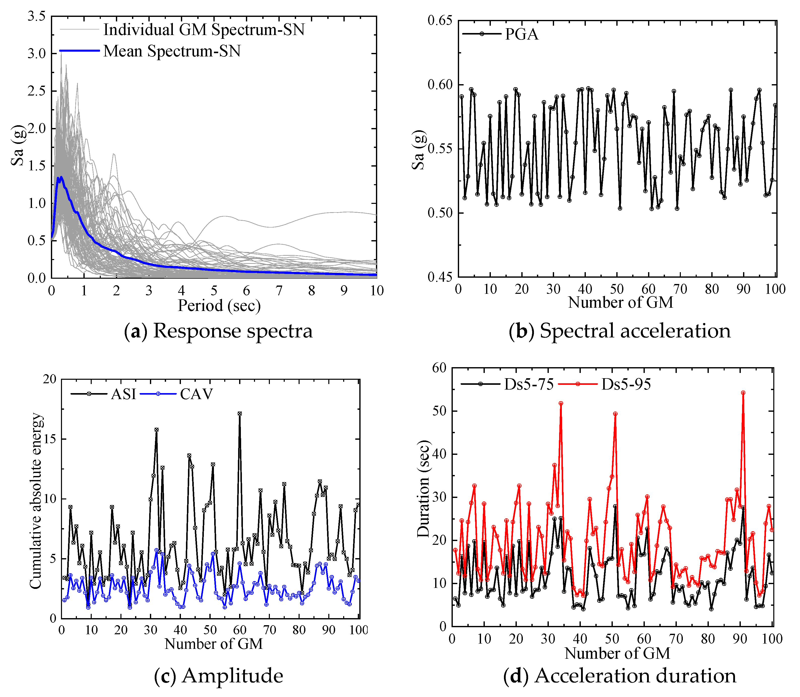
From the regional view, each bridge undertakes different ground motions in the same earthquake scene. Analysis of recorded signals from installed sensors or nearby seismographs could provide the time-history and detailed characteristics of the ground motions. In addition to considering the structural and material uncertainties, the ground motion uncertainties should also be fully considered. Earthquake ground motion is typically characterized by three main aspects: peak effect, response spectrum and acceleration duration [30]. This study selects eight IMs ($G_1~G_8$) to represent these three aspects in the seismic damage state evaluations. PGA and cumulative absolute energy (CAV) are selected to represent the peak effect of ground motion. Acceleration spectrum intensity and spectral acceleration, at the periods of 0.5, 1, and 3 s, are used to show the spectrum intensity characteristics. 5–75% and 5–95% significant durations are chosen as the representatives of time history characteristics. The definitions of these eight selected IMs are listed in

Table 3. Selected intensity measures.

Variables	IM	Definition
$G_1$	$S{a}_{0.5}$	Spectral acceleration at the period of 0.5
$G_2$	$S{a}_1$	Spectral acceleration at the period of 1
$G_3$	$S{a}_3$	Spectral acceleration at the period of 3
$G_4$	$PGA$	Peak ground acceleration
$G_5$	$ASI$	Acceleration spectrum intensity $\mathrm{ASI}={\int }_{0.1}^{0.5}SA\left(T\right)dT$
$G_6$	$CAV$	Cumulative absolute energy $\mathrm{CAV}={\int }_0^{t_{max}}\left|a\left(t\right)\right|dt$
$G_7$	$D{s}_{5-75}$	5–75% significant duration: Intervals between the times where 5% and 75% of ${\int }_0^{t_{max}}a{\left(t\right)}^{2}dt$ obtains.
$G_8$	$D{s}_{5-95}$	5–95% significant duration: Intervals between the times where 5% and 95% of ${\int }_0^{t_{max}}a{\left(t\right)}^{2}dt$ obtains.

.

The ground motion suite used in this study should be informative considering the established 672,000 numerical models. It contains 1000 ground motions that are developed from the Pacific Earthquake Engineering Research (PEER) ground motion database. The PGAs of these 1000 ground motions are evenly distributed between 0 g and 1.0 g, and there are 100 ground motions contained in every 0.1 g interval. Among them, ground motions with PGA lower than 0.4 g are natural ground motions, while the other 600 ground motions are scaled ground motions. Since the ground motions with high PGA are rare in the PEER database, they are scaled from the other natural ground motions to populate sufficient response data for the strong earthquake scene. The IMs of selected ground motions with PGA between 0.5 g to 0.6 g is illustrated in Figure 4. This study randomly pairs 672,000 numerical models with these 1000 ground motions, in both longitudinal and transverse excitations.

4. Vibration-Based Seismic Damage State Evaluation Methodology

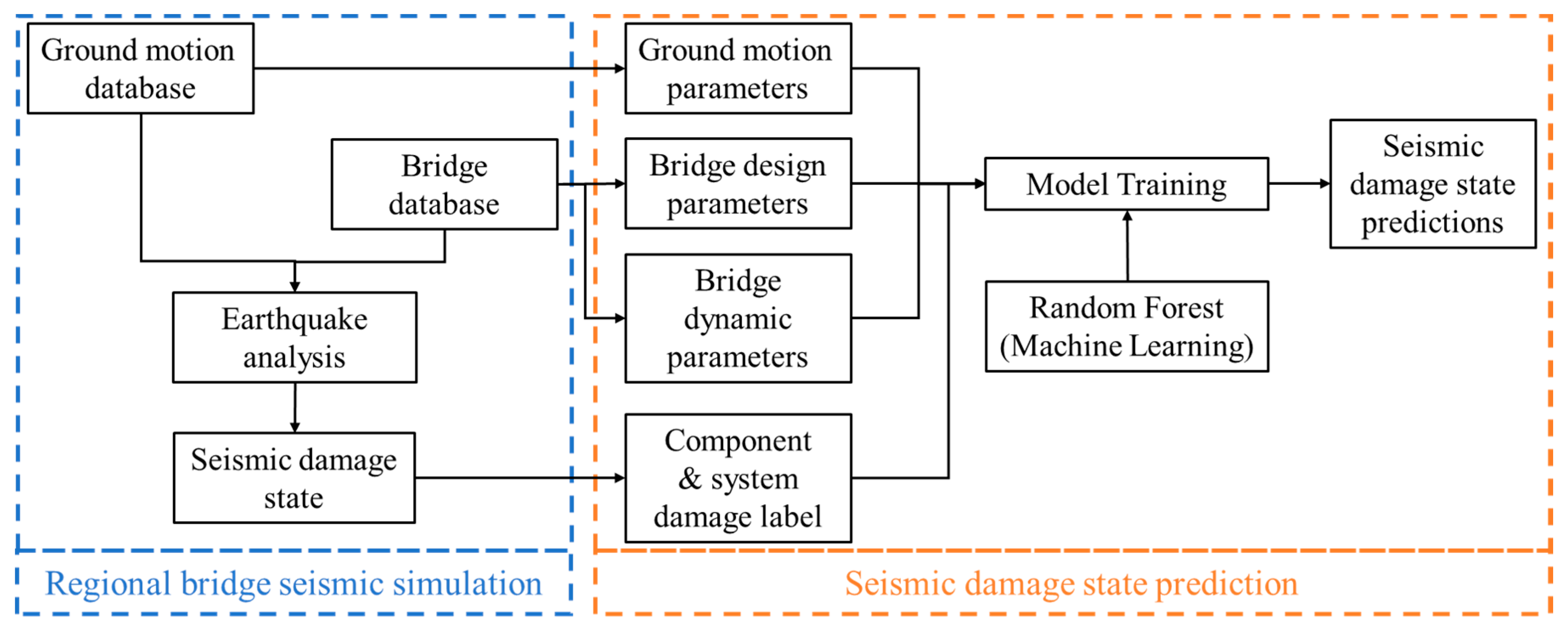
There are two main stages in the proposed evaluation frameworks, including the regional bridge seismic simulation stage and the seismic damage state evaluation stage. The framework for vibration-based seismic damage state evaluations is represented in Figure 5. The seismic simulation stage aims to label the structural seismic damage state for a certain bridge–earthquake pair, and it provides the labeled dataset for the following supervised model training. In the evaluation stage, the labeled 672,000 bridge–earthquake pairs are split randomly in this study into a training set (70%) and a test set (30%). The RF is trained with the training set to minimize the prediction error. The evaluation of the model using the test set informs the prediction performance and prevents overfitting. This study uses the cross-validation strategy to evaluate predictive models. In practice, the training set is randomly partitioned into n equal-sized subsamples. Of the n subsamples, a single subsample is retained as the validation data for testing the model, and the remaining n–1 subsamples are used as training data. The cross-validation process is then repeated n times, with each of the n subsamples used exactly once as the validation data. The n results from the folds can then be averaged to produce a single estimation. The advantage of this method is that all observations are used for both training and validation, and each observation is used for validation exactly once. The ideal trained models are expected to imply the general law of structural seismic damage, and are effectively generalized to other regional bridges.

4.1. Random Forest

RF is an ensemble machine learning method operated by constructing a large number of decision trees (DT). Unlike DT, which uses all features to generate a tree-like graph for classification, RF uses an effective “feature bagging” learning algorithm, which combines the random feature selection and bagging techniques. If one or a few features are very strong predictors for the target output, this subset of features will be selected to construct a tree-like classification graph sample. This kind of sample is known as the bootstrap sample. Using bagging techniques, these models are fitted with the above bootstrap samples and combined by voting. RF improves stability and accuracy, reduces variance, and helps to avoid overfitting.

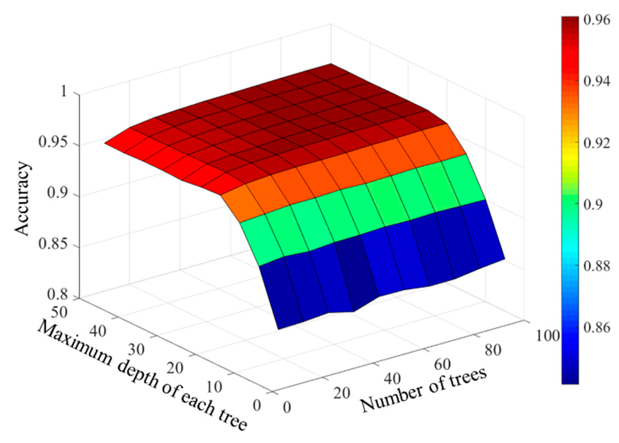
With the size and nature of the training set, an optimal number of trees are determined by bootstrap aggregating or bagging. By averaging the predictions from the individual regression trees, the RF prediction can be expressed as:

$$\widehat{f}\left(x\right)=\frac{1}{T}{{\displaystyle \sum }}_{t=1}^T{f}_t\left(x\right)$$

(1)

where $\widehat{f}\left(x\right)$ denotes the RF prediction from the total of $\mathrm{T}$ trees, and $f_t\left(x\right)$ denotes the prediction of each individual tree with the input $x$. Additionally, an estimate of the uncertainty of the prediction can be made as the standard deviation of the predictions from all the individual trees, and can be expressed as:

$$\sigma =\sqrt{\frac{{\sum }_{t=1}^T{\left(f_t\left(x\right)-\widehat{f}\left(x\right)\right)}^2}{T-1}}$$

(2)

4.2. Component Demands and Damage State Classification Labeling

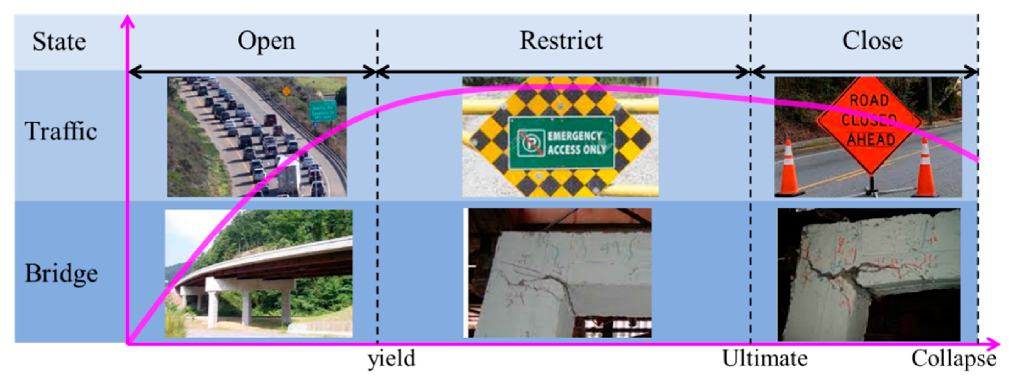
RF is a supervised learning algorithm, which infers the function between input features and output results based on the labeled training data. Following the material performance and bridge design codes, this study suggests three damage states for each bridge component and the whole bridge system, illustrated in Figure 6. The component demand obtained from the nonlinear seismic analysis of the bridges is compared with their capacities, and three damage states are defined as listed in

Table 4. Limit states definition.

State	Open	Restrict	Close
Traffic influence	Open to normal public traffic	Only for emergency and limited vehicles	Closed to all vehicles
Structural damage	No or minor cracks	Cover concrete spalling Core concrete and rebar yield function intact	Core concrete crushing collapse or nearly collapse out of function
Materials performance	$\epsilon \le {\epsilon }_o$	${\epsilon }_0<\epsilon <{\epsilon }_u$	$\epsilon \ge {\epsilon }_u$

, where $\epsilon$ denotes the structural seismic response, ${\epsilon }_o$ denotes the yield strain, and ${\epsilon }_u$ denotes the ultimate strain. Since the seismic demand value of each bridge component in the regional scale is different, this paper only gives the principle of classifying the seismic damage states.

The defined damage states are associated with material performance, structural damage and regional traffic influence. This paper selects five bridge components to make the seismic damage state evaluation. For abutments, the stiffness of longitudinal direction (AbutX) and transversal direction (AbutY) are different, and the yield points and ultimate points are determined via the soil condition and previous research. For bridge bearing (Bear), since it is assumed to be a perfectly elastic model, displacement controls the damage states. Bridge columns (Column) play an important role in seismic analysis. Typical sectional moment-curvature analyses for 672,000 samples are carried out; at the yield point, the built-in rebars start to yield, and cover concrete begins spalling; at the ultimate point, core concrete crashes. The damage state of beam unseating (Beam) is defined via the bridge transverse structure configuration. The whole bridge system is considered as a series system of these five components, and the damage state of the system is determined via the most damaged component.

4.3. Predict Performance Indicators

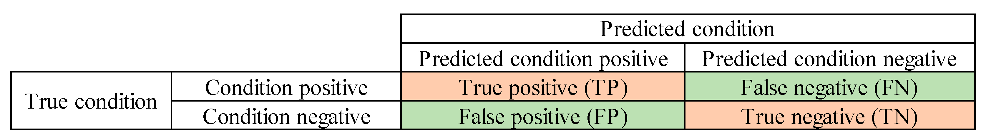
To establish a predictive model for classifying the seismic damage state of components and bridge systems, the RF algorithm is carried out as mentioned in Section 4.1. The confusion matrix is a table for the visualization of the predicted performance, in which each row of the matrix depicts the cases in an actual class, while each column depicts the cases in a predicted class. It is usually constructed with $n$ rows and $n$ columns, where $n$ equals the number of classes. There are four kinds of classification of the analytic results, including true positives (TP), true negatives (TN), false positives (FP) and false negatives (FN), shown in Figure 7. TP and TN are the outcomes where the model correctly predicts the positive and negative class, respectively. FP and FN are two kinds of prediction error, indicating that the model incorrectly predicts the positive and negative class, respectively.

The efficiency of the predictive model is evaluated using the Accuracy, Precision, Recall and F₁-score ($F_1$) of the test data set. Accuracy is the most intuitive performance indicator; it defines a ratio of correctly predicted conditions to the total conditions. Accuracy is a good performance indicator only when FP and FN have a similar cost. Precision defines the ratio of correctly predicted positive conditions to the total predicted positive conditions. In other words, Accuracy denotes the closeness of the predictions to the target value, while Precision denotes the closeness of the predictions to each other. Recall defines the ratio of correctly predicted positive conditions to all conditions in a true condition. $F_1$ denotes the weighted average of Precision and Recall. It is usually more useful in an uneven class distribution [30]. Since the damage state distributions of each component are extremely uneven, $F_1$ is an important indicator in this study. The equations of the above indicators are listed below:

$$Accuracy=\left(TP+TN\right)/\left(TP+FP+TN+FN\right)$$

(3)

$$Precision=TP/\left(TP+FP\right)$$

(4)

$$Recall=TP/\left(TP+FN\right)$$

(5)

$$F_1=2\times Precision\times Recall/\left(Precision+Recall\right)$$

(6)

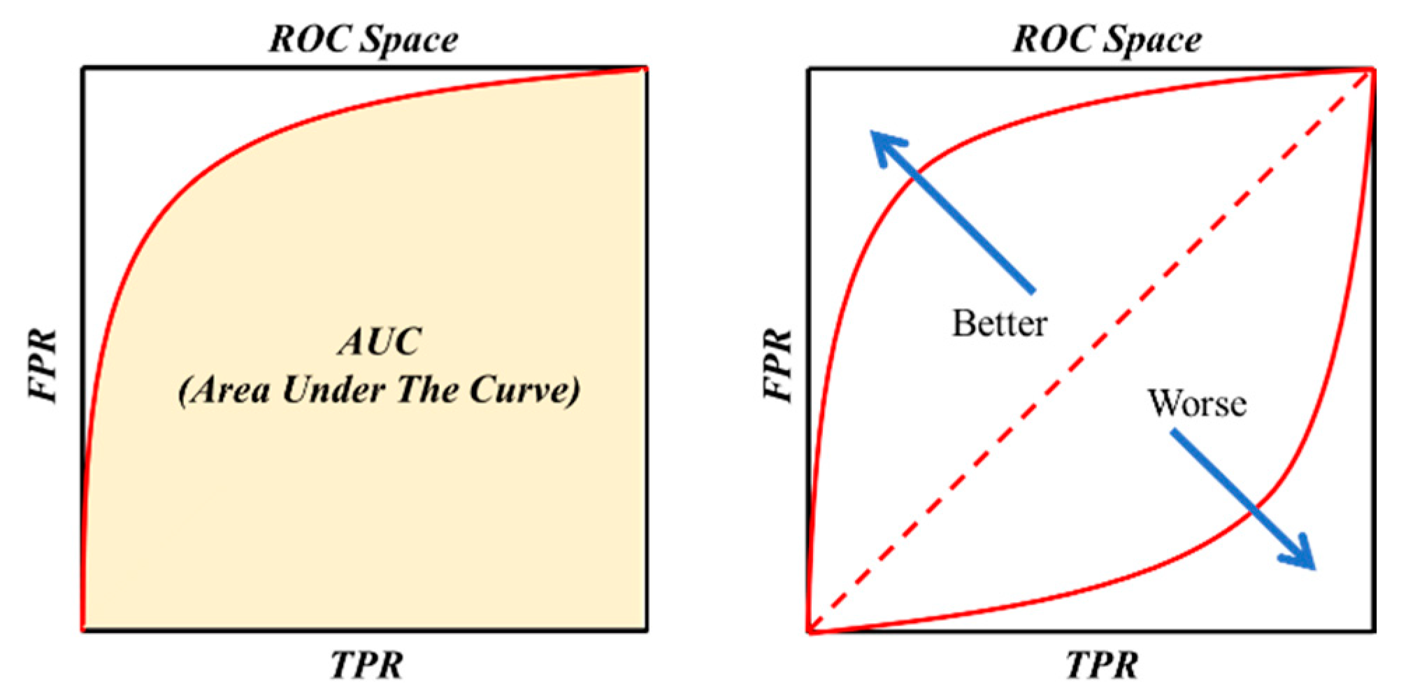
The receiver operating characteristic curve (ROC Curve) and area under the curve (AUC) are performance indicators that depict the diagnostic ability of the established classifier. ROC Curve defines a probability curve plotting the true positive rate (TPR) against the false positive rate (FPR), at various setting values. An excellent prediction method would approach the point at the upper left corner of the ROC space, representing no FN and FP. Under this circumstance, the associated AUC is near to 1, as shown in Figure 8. The equations of TPR and FPR are listed below:

$$TPR=TP/\left(TP+FN\right)$$

(7)

$$FPR=FP/\left(FP+TN\right)$$

(8)

5. Application of Proposed Methods to the Established Regional Bridges

5.1. Prediction Accuracy of Traditional and Proposed Methods

These models are established and implemented on an open-source machine learning library scikit-learn 0.20.3 in Python 3.7. The computer used for training these models is built with an i7-8700K CPU and a 16 GB memory. The total training time for the six models (AbutX, AbutY, Bear, Column, Beam and System) is 79.88 s and 76.55 s, for the traditional method and the proposed method, respectively.

Using the traditional method and proposed method, the seismic damage states of concrete beam bridges can be predicted. In the traditional method, the material and boundary stiffness parameters ($R_8~R_{12}$) are used to determine the bridge material’s strength and boundary condition. Usually, these parameters are quite hard to obtain for an in-service bridge, and seismic damage states are predicted with the original design condition. However, the proposed method uses the real-time dynamic characteristics instead of original material and boundary stiffness parameters to determine the bridge condition. It is quite convenient for monitored bridges to measure these frequencies ($P_7~P_{11}$).

This study compares the prediction accuracy between traditional methods and proposed methods for two bridge conditions, that is, the intact condition and the 20% deterioration condition. In the deteriorated models, the stiffness and ultimate strength of concrete and reinforcement bars in the bridge column are assumed to have undergone 20% deterioration. In the boundary conditions, it is assumed that the stiffness of the bearing and the abutment are reduced by 20%.

Table 5. Accuracy comparison of traditional and proposed methods for intact bridges.

Methods	AbutX	AbutY	Bear	Column	Beam	System
Traditional	96.01%	95.25%	88.82%	96.67%	93.87%	94.54%
Proposed	96.27%	95.87%	89.61%	96.77%	94.23%	94.63%

illustrates the results of the intact condition; since the material strength and boundary stiffness are not damaged, the accuracy of both traditional methods and proposed methods accounts for over 90%. As for the results of the deteriorated bridges shown in

Table 6. Accuracy comparison of traditional and proposed methods for bridges with 20% deterioration.

Methods	AbutX	AbutY	Bear	Column	Beam	System
Traditional	77.52%	81.19%	72.46%	78.19%	76.22%	80.33%
Proposed	93.82%	94.95%	89.06%	95.19%	93.12%	93.24%

, the accuracy of traditional methods decreases to about 75%. The original design materials and boundary parameters greatly affect the prediction accuracy. However, the proposed method still possesses a high prediction accuracy of 95%. Since the monitored dynamic characteristics reflect the real-time bridge conditions, the proposed methods perform well in both intact bridges and deteriorated bridges.

5.2. Performance of Proposed Evaluation Methods

As explained above, the confusion matrix ($\mathit{C}$) shows a table of the actual class versus predicted class, where $C_{ij} \left(i=1:3, j=1:3\right)$ denotes the number of observations known to be in class $i$, but predicted to class $j$. Therefore, the diagonal elements in $\mathit{C}$ indicate the observations that are correctly classified by the proposed seismic damage evaluation method, and the off-diagonal elements indicate the observations that are incorrectly predicted. In Figure 9, the dark red represents the associated elements that are most likely to be predicted. The performance of the proposed method in the classification prediction is also evaluated with Precision and Recall, which are given in the fourth row and column in $\mathit{C}$, respectively. High precision and recall rates represent the ability of the proposed method to accurately predict the seismic damage states. For example, Figure 9a illustrates the seismic damage state evaluation results for the longitudinal abutment; the diagonal elements are all colored with dark red, indicating that most of the damage states are correctly predicted. “Open” state and “Restrict” state account for high precision and recall rate, while the “Close” state has a slightly lower rate. As for other components and bridge systems, the proposed method also exhibits a high accuracy, precision and recall rate.

Figure 10 shows the damage state distribution for bridge components and systems in the test dataset. It is seen that these distributions are quite uneven, especially for AbutX, AbutY, Beam, and System. They are mainly distributed in one damage state, and the value of this damage state is larger than the other damage states. Since $F_1$ can comprehensively evaluate the prediction performance for uneven class distributions with weighted precision and recall rates, this study summarizes the score of each bridge component and system, shown in Figure 11. For AbutY, Beam and System, the score of the proposed method reaches over 90%. The lowest score appears in the “Close” state of AbutX, which accounts for 79.47%. In other words, predicting the seismic damage states with the proposed methods is a reliable approach.

The ROC Curve is a tool for testing the generalization performance of established models. In machine learning, generalization is a term used to describe a model’s ability to react to new data. A trained model with good generalization performance could effectively digest new data and make accurate predictions. The best classification model yields a point in the upper left area of ROC space, and the related AUC is 1. Figure 12 shows the ROC Curves and related AUC for each bridge component and system. It is observed that proposed seismic damage state evaluation methods exhibit a great generalization performance for all components. Among them, the lowest area is 0.9719, appearing in the “Close” state of Bear, and others are around 0.99. From the zoomed spaces, each ROC curve approaches the top left corner (0,1). These strong generalized models may accurately predict the seismic damage states of new regional bridges.

The sensitivity of the prediction accuracy of the proposed method, with the number of trees and the maximum depth of each tree is further evaluated in this study, as shown in Figure 13. Since the tuning mechanism of RF is the same for each component and bridge system, this study selects the bridge system to evaluate the sensitivity of the prediction accuracy. It is seen from the figure that the maximum depth of each tree has a greater impact on the prediction accuracy than the number of trees. After a depth of 20 for each tree, the prediction accuracy remains constant in the current study, and the training time constantly increases. Note that the confusion matrix, precision, recall and ROC Curve presented in previous sections correspond to a depth of 20 for each tree, displaying a trade-off between time consumption and prediction performance.

5.3. Significant Parameters Identification

The identification of significant parameters can help bridge engineers and stakeholders to identify critical parameters for seismic design and retrofit. In the established machine learning models, it is important to accurately predict the seismic damage states with correctly estimated and identified significant parameters. The relative significance of each parameter ($k_i$) could be calculated, and they are normalized with the min–max scaling principle in Equation (9), where ${\mu }_i$ denotes the normalized importance value. By accumulating the relative importance from the most significant parameters, the accumulated significant value is calculated with Equation (10). When it reaches or exceeds 95%, the relevant cumulative parameters are identified as significant parameters.

$${\mu }_i=\frac{k_i-min\left(k_1, k_2,\dots ,k_i,\dots ,k_n\right)}{max\left(k_1, k_2,\dots ,k_i,\dots ,k_n\right)-min\left(k_1, k_2,\dots ,k_i,\dots ,k_n\right)}$$

(9)

$$Accumulat{e}_n={\sum }_{j=1}^n{k}_j$$

(10)

Figure 14 shows the significant sequence of parameters, normalized significant values, and identified significant parameters, for each component and bridge system. Although each component and bridge system are identified with different significant parameters, all the proposed dynamic characteristics ($P_7~P_{11}$) are identified. Moreover, some design parameters ($P_1~P_6$) are out of the significant parameters. It can be seen that the seismic damage states can be precisely determined with the measured dynamic characteristics and IMs for the monitored bridges, and some insignificant design parameters can be neglected in the estimations. The proposed dynamic characteristic parameters, which reflect the structural real-time conditions, have a great influence on the seismic damage state. This is consistent with the fact that the structural dynamic characteristics contain some information on structural configuration and conditions. As for bridge design parameters, skew angle ($P_6$) has a significant influence on the damage state of all components and bridge systems, and diameter of Column ($P_4$) ranks the top in the significant parameters concerning the column. These correspond to the fact that skew bridges suffer more severe earthquake damages than straight bridges, and the increase of the column configuration increases the seismic resistance of the bridge column. The most significant parameters of ground motion intensities are $PGA$ ($G_4$) and $S{a}_1$ ($G_2$). With these identified significant parameters, the RF-based evaluation models can be simplified.

6. Conclusions

Regional transportation networks play an important role in urban areas. The efficient seismic evaluation of regional bridges can identify the potential damage of components before the earthquake, and guide the recovery operation after an earthquake. With the aid of a structural health monitoring system (SHMS), the bridge’s real-time condition can be accurately identified. SHMS could also identify ground motions that are exerted on the monitored bridges during the earthquake. Based on the measured information and some bridge design parameters, this paper proposes an effective seismic damage evaluation method for regional monitored concrete beam bridges with machine learning techniques.

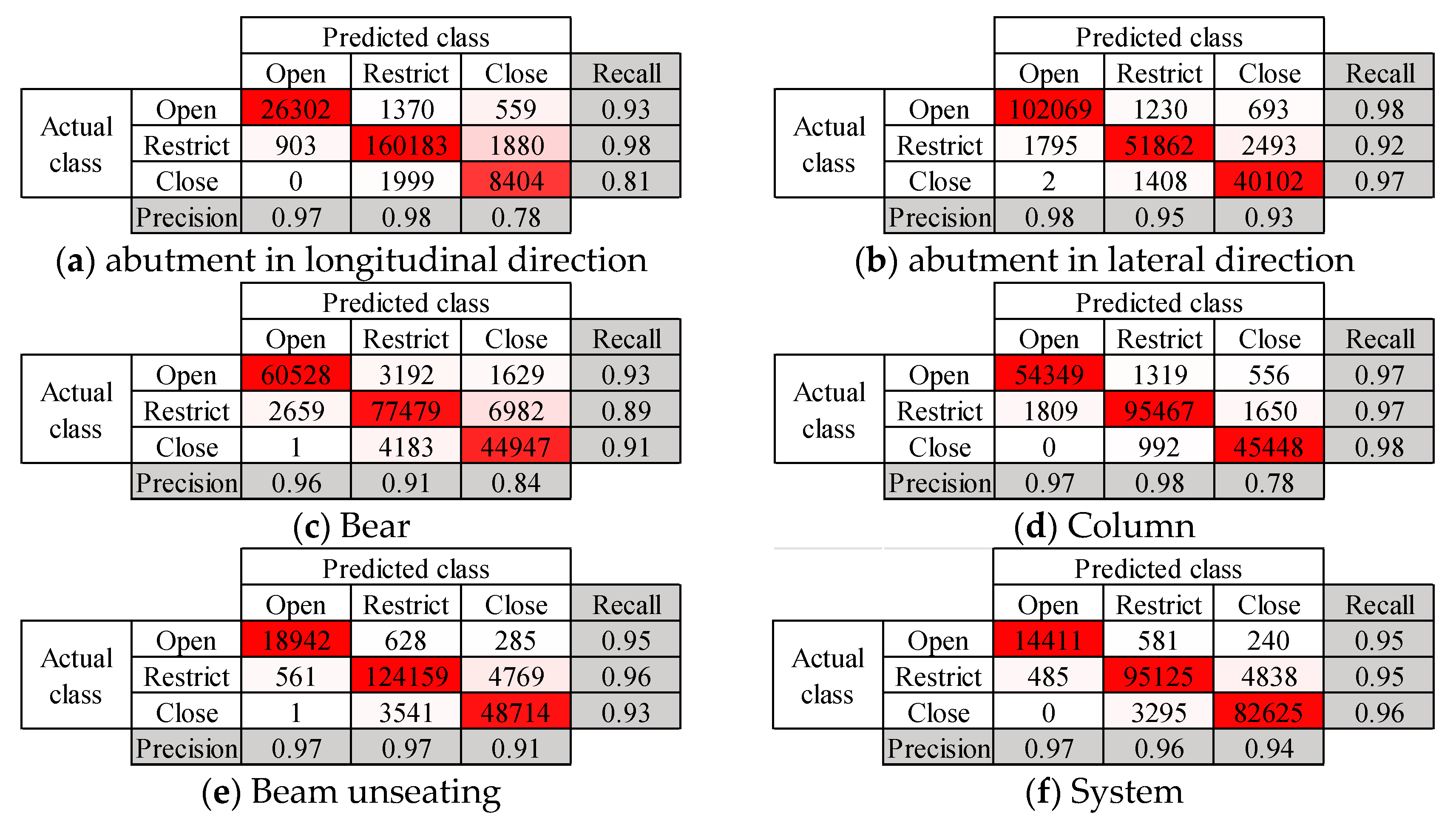
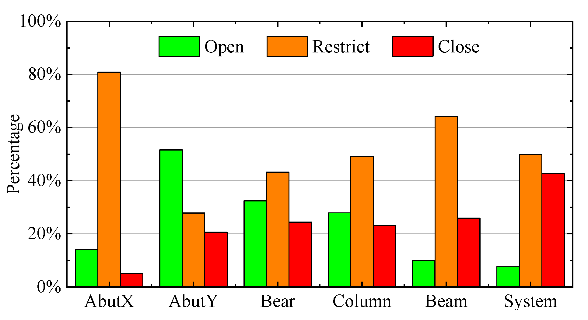
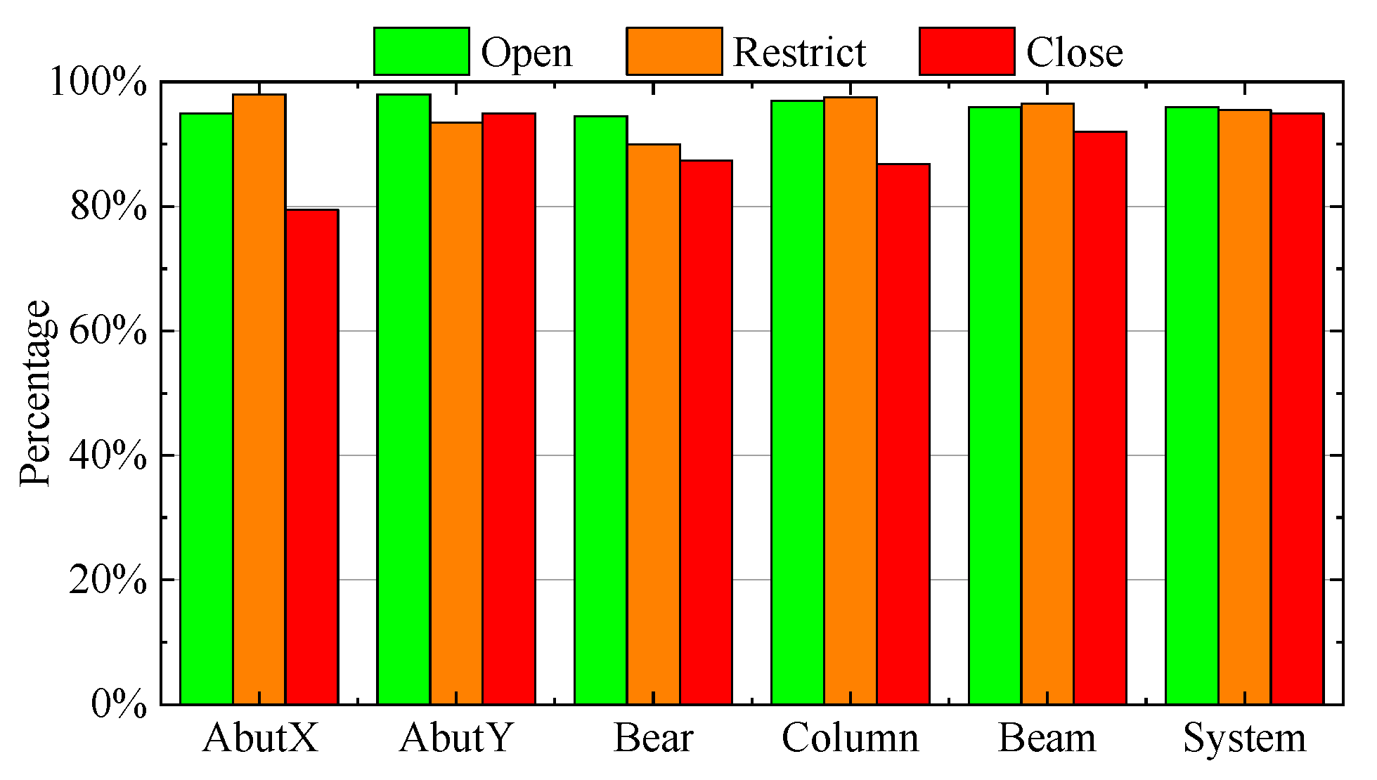
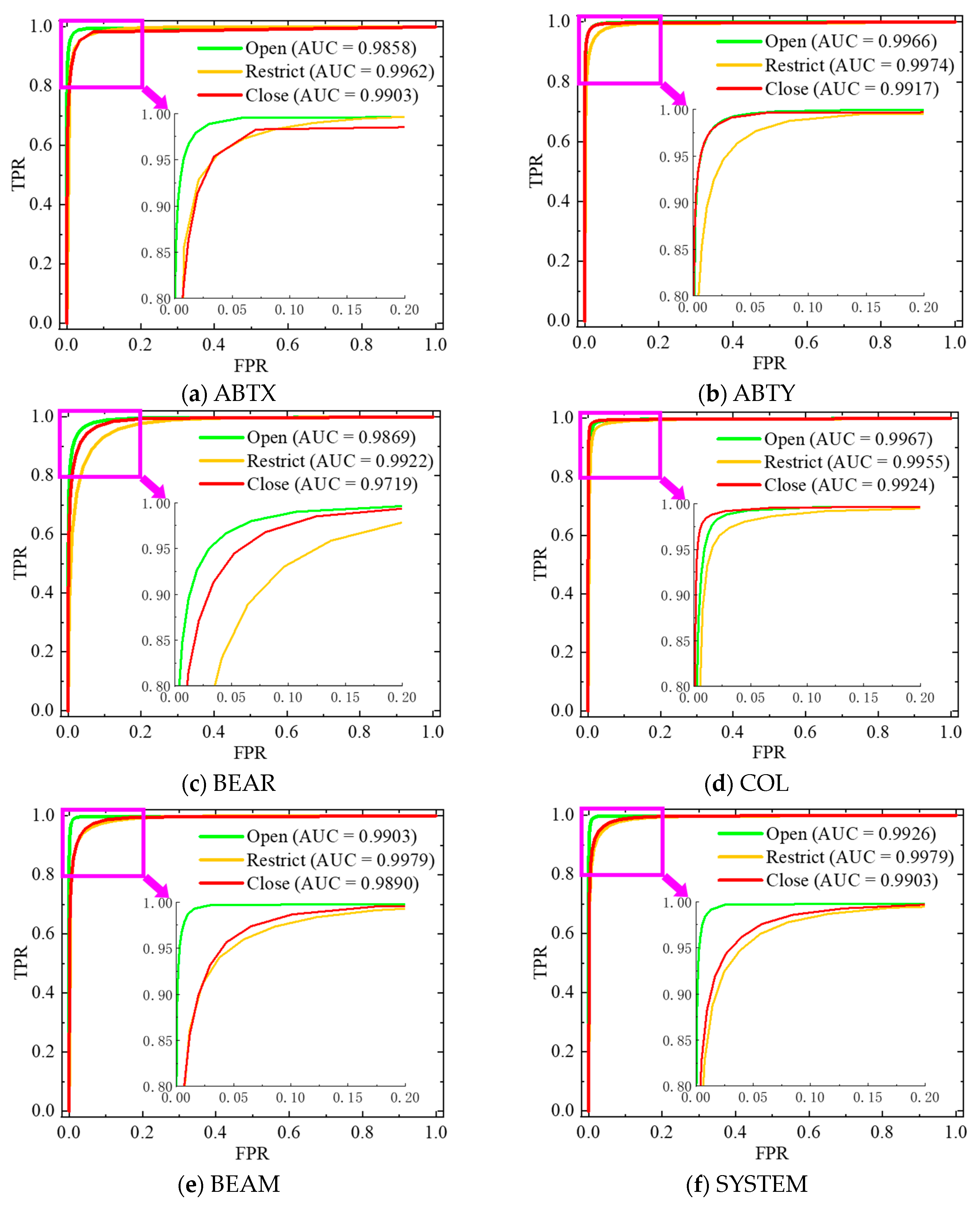
The proposed seismic damage evaluation method is demonstrated for short- and medium-span beam bridges, which are the dominant bridge classes on a regional scale. 672,000 bridge numerical models are probabilistically generated, representing the structural and material diversity of regional beam bridges, and 1000 ground motions are developed to representing the regional ground motion diversity. The non-linear time history analysis of the bridges is carried out to estimate the seismic damage state of selected bridge components and systems. The seismic damage states are labeled with three tags: Open (structural safe), Restrict (open for emergencies) and Close (collapse or the potential to collapse). Using the selected bridge design parameters, bridge dynamic parameters, intensity measures and associated labeled damage states in the dataset, the models are trained with RF. The performance of the proposed machine learning models is explored in this study. RF can predict the seismic damage states with an accuracy ranging from 89% to 97%, depending on the bridge components and system. The precision, recall and F₁-score of most bridge components and systems account for at least 90%. The area under the receiver operating characteristic curve for bridge components and systems yields over 0.99. It is noted from these performance indicators for bridge components and systems that RF has great performance potential in evaluating the seismic damage states of regional beam bridges.

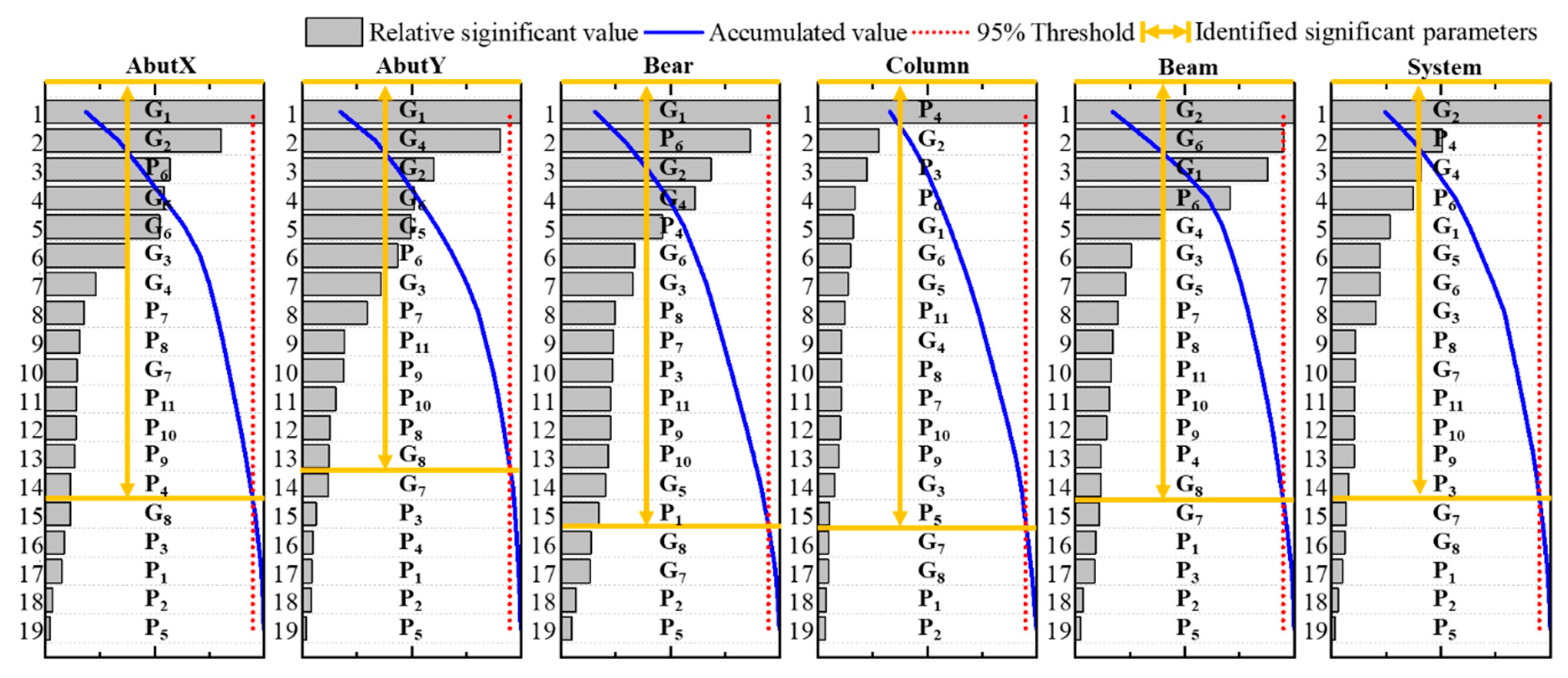
RF is also applied to identify the significant parameters of each bridge component and system in the seismic damage state evaluation. Since the measured structural dynamic characteristics could reflect the structural configuration and real-time conditions, most of them are proved to have a significant influence on the seismic damage state, while some bridge design parameters are neglected. Along with these bridge dynamic parameters, this study also indicates that the skew angle and some ground motion intensities have a major impact on seismic damage states. It is of great importance to have the multi-parameter seismic fragility models available to assess the damage risk and loss of regional bridges. The proposed RF-based damage evaluation method could rapidly and precisely evaluate the seismic damage states. Since the numerical models established in this study are based on the Chinese bridge design code and Chinese official recommended standard drawings, the findings in this study should be carefully applied in other areas. In addition, further studies will apply the proposed method to other area bridges, and compare the seismic characteristics of bridges in different regions.