Highly Efficient and Robust Grid Connected Photovoltaic System Based Model Predictive Control with Kalman Filtering Capability

Abstract

Renewable energy sources, especially photovoltaic (PV) ones, are gaining more and more interest due to the predicted lack of conventional sources over the coming years. That shortage is not the only concern, as environmental issues add to this concern also. Thus, this study proposes two-stage PV grid connected system, which is supported with extended Kalman filter (EKF) for parameter estimation. In the first stage, maximum power point tracking (MPPT) for the boost converter is accomplished using new MPPT method in which the switching state of the converter is directly generated after the measurement stage, so it is called direct switching MPPT technique. This technique is compared with the conventional finite control set model predictive control (FCS-MPC) method, where the design of the cost function is based on minimizing the error between the reference and the actual current. The reference current is obtained by employing perturb and observe (P&O) method. In the second stage, the two-level inverter is controlled by means of model predictive control (MPC) with reduced computation burden. Further, to overcome the parameter variations, which is a very common problem in MPC applications, an extended Kalman filter is utilized to eliminate the control algorithm’s dependency on the parameters by providing an efficient estimation. After the inverter, an RL filter is inserted to guarantee the quality of the currents injected into the grid. Finally, the system is validated using Matlab under different operating conditions of atmospheric variation and parameter changes.

1. Introduction

Photovoltaic (PV) energy sources are very promising due to several advantages over the conventional sources. PV sources provide clean, silent, friendly, naturally abundant and emissions-free energy to the installed systems [1]. These systems can be implemented with different topologies and control methodologies. However, they can be mainly classified into two main categories, including standalone and grid connected applications [2,3]. In the standalone systems, a DC–DC converter is utilized between the PV source and the DC load for the purpose of maximum power point tracking (MPPT) [4]. Actually, some systems use a direct coupling technique between the load and the source, but this method installs a lot of panels to provide the necessary energy to the load [5]. Additionally, and because of the night hours, the storage element is mandatory in case of the standalone schemes [6]. Batteries are a very common solution to this issue, but they require frequent replacement [7], which increases the overall system cost, especially for low power applications. Thus, grid-connected topologies are preferred; they can be implemented by directly coupling the inverter to the grid without including the DC-DC converter stage [8,9]. Consequently, that is called the single stage topology. However, and due to the variable atmospheric conditions, the two stage inverter topology is very common [10,11]. The DC–DC converter stage provides regulation to the PV source voltage [9,12]. In fact, it boosts the voltage, and hence this widens the operating voltage range of the system. Furthermore, it separates the MPPT control strategy from active and reactive power inverter control. This greatly simplifies the overall control methodology and enhances the system stability [13,14].

In the DC–DC stage, the maximum power should be extracted from the PV source [15]. The converter in this stage operates as a matching circuitry because of the nonlinear characteristics of the PV source and also elevates the PV voltage for proper grid connection [16,17]. Many MPPT techniques have been addressed in the literature [18,19,20,21]. Indeed, they differ from each other based on several factors, including methodology, efficiency, tracking speed, required sensors and cost [18,22,23]. The most widespread techniques are perturb and observe (P&O) and incremental conductance (INC) [24]. That is because of the simplicity of implementation. Further, they do not depend on the PV source or system parameters [25]. Recently, and as a result of the continuous development of controllers (microprocessors), advanced techniques, such as the fuzzy logic controller, neural networks, model predictive control (MPC) and optimization techniques, have emerged into the light [26,27]. Optimization techniques or searching algorithms involving particle swarm optimization, genetic algorithm and simulated annealing [28], are applied in nature for systems exposed to partial shading conditions caused by nearby buildings or trees, clouds or even smoke [29]. As a result, the power-voltage (P–V) curve of the PV source exhibits several maxima, so the searching algorithm seeks the global maximum among them [30,31].

Through the inverter stage, the DC energy is converted to AC energy. Moreover, the control strategy in this stage relies on independent control of active and reactive power injected into the grid [12,26]. Several inverter control strategies are implemented in the literature. However, the most popular technique is the voltage oriented control (VOC) [32]. In this method, two cascaded control loops are required. The outer loop (voltage loop), normally associated with the DC-link capacitor voltage, provides the direct axis component of current $\left(I_d\right)$ for the purpose of active power control. Alongside the quadrature axis component of the current $\left(I_q\right)$, this is usually set to zero to operate at a unity power factor conditions. These two components are feed to the inner current loop with a modulator to get the switching signals for the inverter [32,33]. For the sake of decoupling intentions and PI controller design simplicity, the VOC can be implemented with feed forward technique [33,34]. Another common algorithm is the direct power control (DPC) strategy; actually, in this technique the cascaded control methodology of the VOC is avoided [35]. The inverter switching states are selected based on the instantaneous errors between the estimated and reference values of the active and reactive power, and the grid voltage vector position [35,36]. The DPC strategy is executed by means of hysteresis controller and lookup switching table [36,37], and hence there is no need for the modulator.

Recently, and over the past few years, predictive control has gotten more attention and become a very promising control scheme in various power electronics applications [32,38,39]. It can be sorted into three prime branches incorporating the continuous control set, deadbeat and finite control set model predictive control (FCS-MPC) [40]. Both the continuous control set and deadbeat model predictive control need a modulator at the output stage for switching state generation [41]. However, FCS-MPC takes the advantage of limited number of switching actions related to the controlled converter and directly generates the optimal switching state. FCS-MPC can be simply performed by deriving the model of the system under study. Then, the discrete time model of the converter is developed. Further, the predicted control variable is differentiated from its reference value together with other conditions. Finally, the best switching action satisfying the aforementioned constraints will be enforced on the power switches [41,42,43]. Obviously, the model of the system has a great effect on optimizing the FCS-MPC performance [35,40]. This opens the door for combining different observers with FCS-MPC to estimate the parameters of the model and enhance the robustness of the control strategy. Various studies have been carried out using such things as the model reference adaptive system (MRAS) [44,45], the Luenberger observer [46], the disturbance observer [47] and the extended Kalman filter (EKF) [48]. However, these estimators can also be used for state estimation and hence sensorless control strategies [49]. Presently, limited work is done in this area, and that motivated the authors to go after this control strategy, particularly for PV grid connected systems.

In this paper, a two-stage, grid-connected PV system is proposed with an optimized control strategy considering high MPPT efficiency for the boost converter and high robustness for the two-level inverter scheme. Firstly, the maximum power is extracted from the PV source by a new direct switching MPPT algorithm. For investigation, the proposed methodology is compared with the FCS-MPC MPPT [50], which is designed with one step in the horizon, and the cost function is adopted based on the current. Secondly, a modified FCS-MPC is developed to control the inverter, wherein only three iterations are required to initiate the optimum voltage vector, unlike the case of the conventional FCS-MPC, wherein seven iterations are essential. This considerably decreases the required computation time. Further, to enhance the system’s reliability and robustness, and even eliminate the FCS-MPC dependency on the parameters of the scheme, an EKF is employed to monitor and observe the parameters for the objective of online correction of potential variations. Finally, the behavior of the system is validated with simulation results using Matlab under different operating conditions and compared with the conventional FCS-MPC algorithm.

The rest of this paper is organized as follows. Section 2 presents the mathematical model of the PV source, boost converter and proposed MPPT. Section 3 describes the conventional and the proposed FCS-MPC algorithms for controlling the two-level inverter. The extended Kalman filter design is explained in Section 4. Finally, simulation results are illustrated in Section 5.

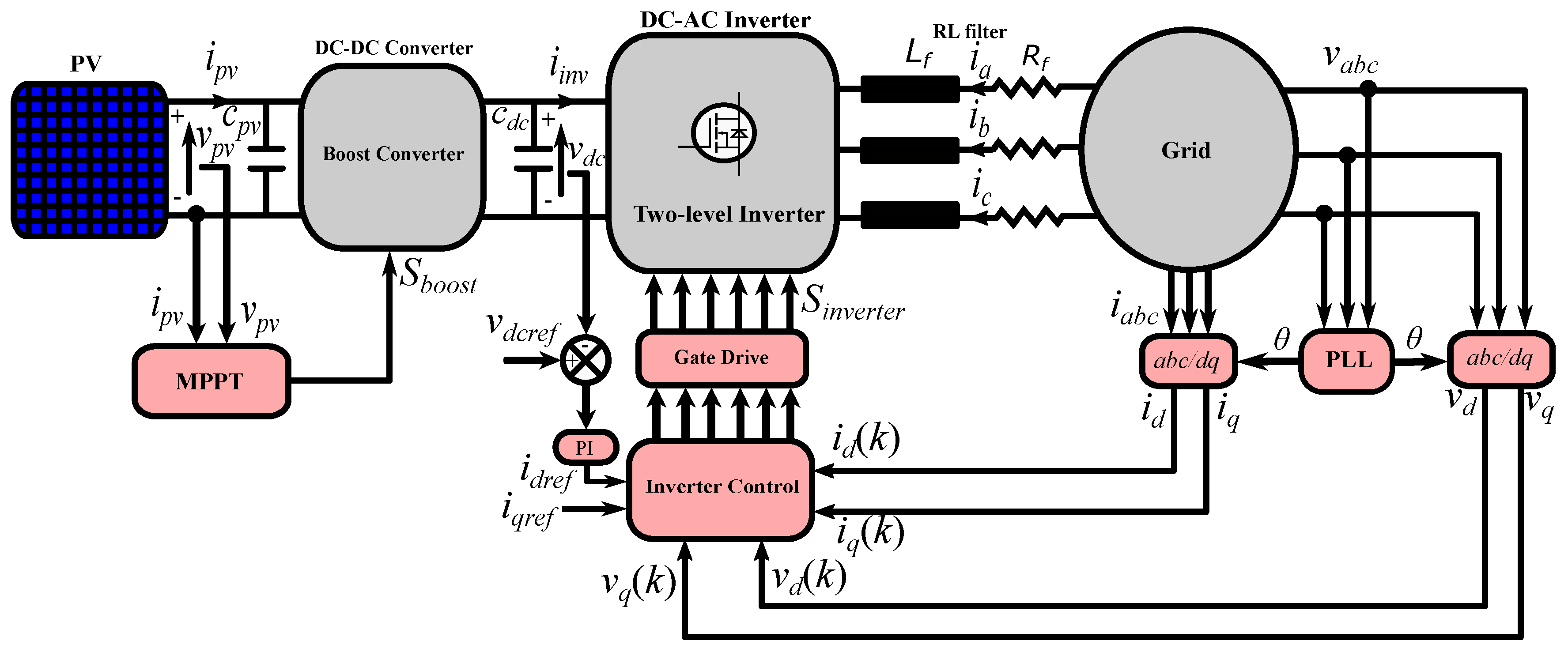
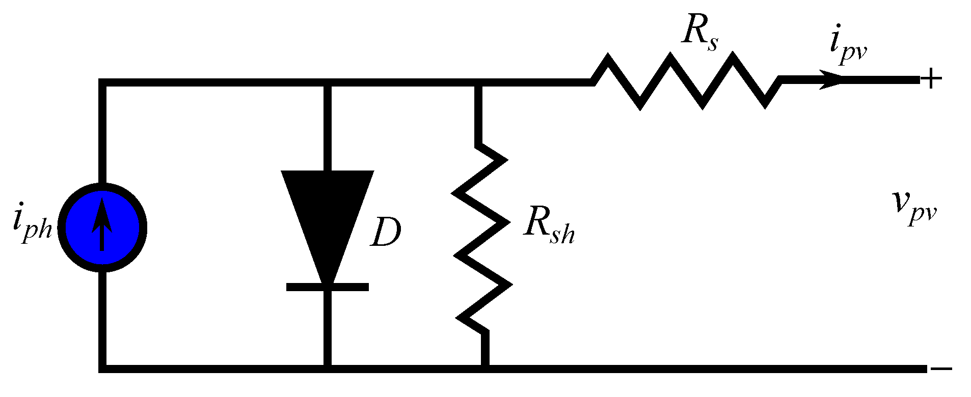
2. PV System Modeling and MPPT

The studied PV system, shown in Figure 1, consists of PV source (PV array), a boost converter, a two-level inverter, an RL filter and the grid. The PV source and the DC-DC converter stage are investigated in the coming subsections.

2.1. PV Array Modeling

The PV cells provide small output voltage, so normally the PV source is available in modules (panels) formed from series cells. The modules can further connected in series and parallel (array) to provide sufficient power to the system. Here, the single diode model is used for describing the behavior of the PV module as [20,51]

$$i_{pv}=i_{ph}-i_o[e^{\left(\frac{v_{pv}+i_{pv}{R}_s}{n{N}_s{v}_t}\right)}-1]-\frac{v_{pv}+i_{pv}{R}_s}{R_{sh}},$$

(1)

where $i_{ph}$ is the photovoltaic current, n is the diode ideality factor, $i_o$ is the diode saturation current, $R_s$ is the module series resistance, $R_{sh}$ is the module shunt resistance, $v_t=kT/q$ is the thermal voltage, $N_s$ is the number of series cells in the module, $i_{pv}$ is the terminal current and $v_{pv}$ is the terminal voltage. The electrical circuit that describes this model is shown in Figure 2.

Further, the characteristics of the module KC200GT [52] chosen for simulation are shown in Figure 3, Figure 4, Figure 5 and Figure 6, where the P–V and the I–V characteristics are illustrated at different atmospheric conditions of radiation and temperature.

2.2. Boost Converter Model

The objective of the boost converter in PV systems is to interface the PV source with the two-level inverter, and to boost the voltage of the array to a convenient value for grid connection. The boost converter has two modes of operation, which are specified by the power switch cases on and off. Figure 7 shows the two modes of the converter, where its behavior can be formulated as follows:

When the switch is off:

$$\frac{d{i}_l}{dt}=\frac{1}{L_b}(v_{pv}-v_{dc}),$$

(2)

$$\frac{d{v}_{dc}}{dt}=\frac{1}{c_{dc}}(i_l-i_{inv}),$$

(3)

where $i_l$ is the inductor current, $v_{dc}$ is the capacitor voltage, $L_b$ is the boost converter inductance, $i_{inv}$ is the inverter current and $c_{dc}$ is the coupling capacitor value (between the boost and the two-level inverter).

And when the switch is ON:

$$\frac{d{i}_l}{dt}=\frac{1}{L_b}{v}_{pv},$$

(4)

$$\frac{d{v}_{dc}}{dt}=-\frac{1}{c_{dc}}{i}_{inv}.$$

(5)

Using the state space averaging technique, the boost model can be finalized as

$$\begin{array}{c}\dot{x}=\mathbf{A}x+\mathbf{B}u,\hfill \\ y=\mathbf{C}x+\mathbf{D}u,\hfill \end{array}$$

(6)

where x = [$i_{pv}$ $v_{dc}$]${}^{\mathit{T}}$ is the state vector, u = [$v_{pv}$ $i_{inv}$]${}^{\mathit{T}}$ is the input vector and $y=v_{dc}$ is the output. Further, $\mathbf{A}$, $\mathbf{B}$, $\mathbf{C}$ and $\mathbf{D}$ are the system matrices and are expressed as follows

$$\mathbf{A}=\left[\begin{array}{cc}0& -\frac{1-d}{L_b}\\ \frac{1-d}{c_{dc}}& 0\end{array}\right],\mathbf{B}=\left[\begin{array}{c}\frac{1}{L_b}\\ -\frac{1}{c_{dc}}\end{array}\right],\mathbf{C}=\left[\begin{array}{cc}0& 1\end{array}\right],\mathbf{D}=0,$$

(7)

where d is the duty cycle of the boost converter.

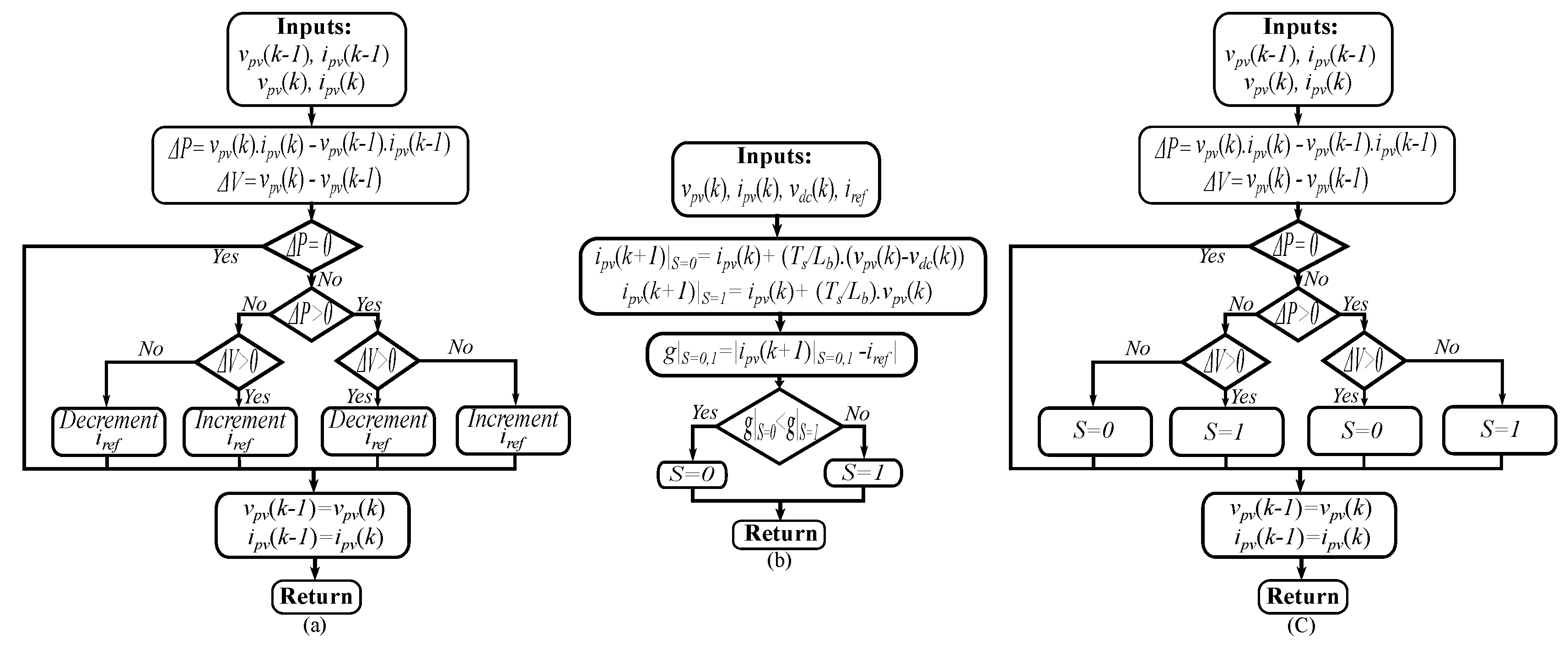
2.3. MPPT Using FCS-MPC

Maximum power point tracking is an essential regulation to capture the obtainable power from the PV source during the variable operating conditions. At this stage, FCS-MPC technique is developed to extract the maximum power from the array. The FCS-MPC requires the discrete-time model of the boost converter, which can be derived from the above-mentioned model (Equations (2)–(5)), and using forward Euler discretization [53]

$$i_{pv}(k+1)=i_{pv}\left(k\right)+\frac{T_s}{L_b}(v_{pv}\left(k\right)-v_{dc}\left(k\right)),$$

(8)

$$v_{dc}(k+1)=v_{dc}\left(k\right)+\frac{T_s}{c_{dc}}(i_{inv}\left(k\right)-i_{pv}\left(k\right)),$$

(9)

$$i_{pv}(k+1)=i_{pv}\left(k\right)+\frac{T_s}{L_b}{v}_{pv}\left(k\right),$$

(10)

$$v_{dc}(k+1)=v_{dc}\left(k\right)-\frac{T_s}{c_{dc}}{i}_{inv}\left(k\right),$$

(11)

where $i_{pv}$≈$i_l$, Equations (8) and (9) are valid when the switch is open. Equations (10) and (11) describe the on state, $T_s$ is the sampling time, k represents the actual sampling instant and $(k+1)$ is the future one.

The design of the cost function is based on the current as

$$g_{S=0,1}=\left|i_{p{v}_{S=0,1}}(k+1)-i_{ref}(k+1)\right|,$$

(12)

where S is the switching state of the boost converter, and $i_{ref}(k+1)$ is the reference current generated from the P&O method. The final scheme for the conventional FCS-MPC MPPT method is shown in Figure 8.

2.4. MPPT Using Direct Switching Technique

Maximum power can be harnessed from the PV source using the well-known direct control method [54,55,56,57], where the duty cycle is directly perturbed in the control algorithm without the need for PI controllers [54,58]. Combining this idea with the FCS-MPC MPPT principle, the duty cycle can be replaced with the converter switching state, as shown in Figure 8. The main advantages of the proposed MPPT are: (1) The avoidance of current predictions and cost function evaluations (i.e., low computational load), and (2) no dependency on system parameters.

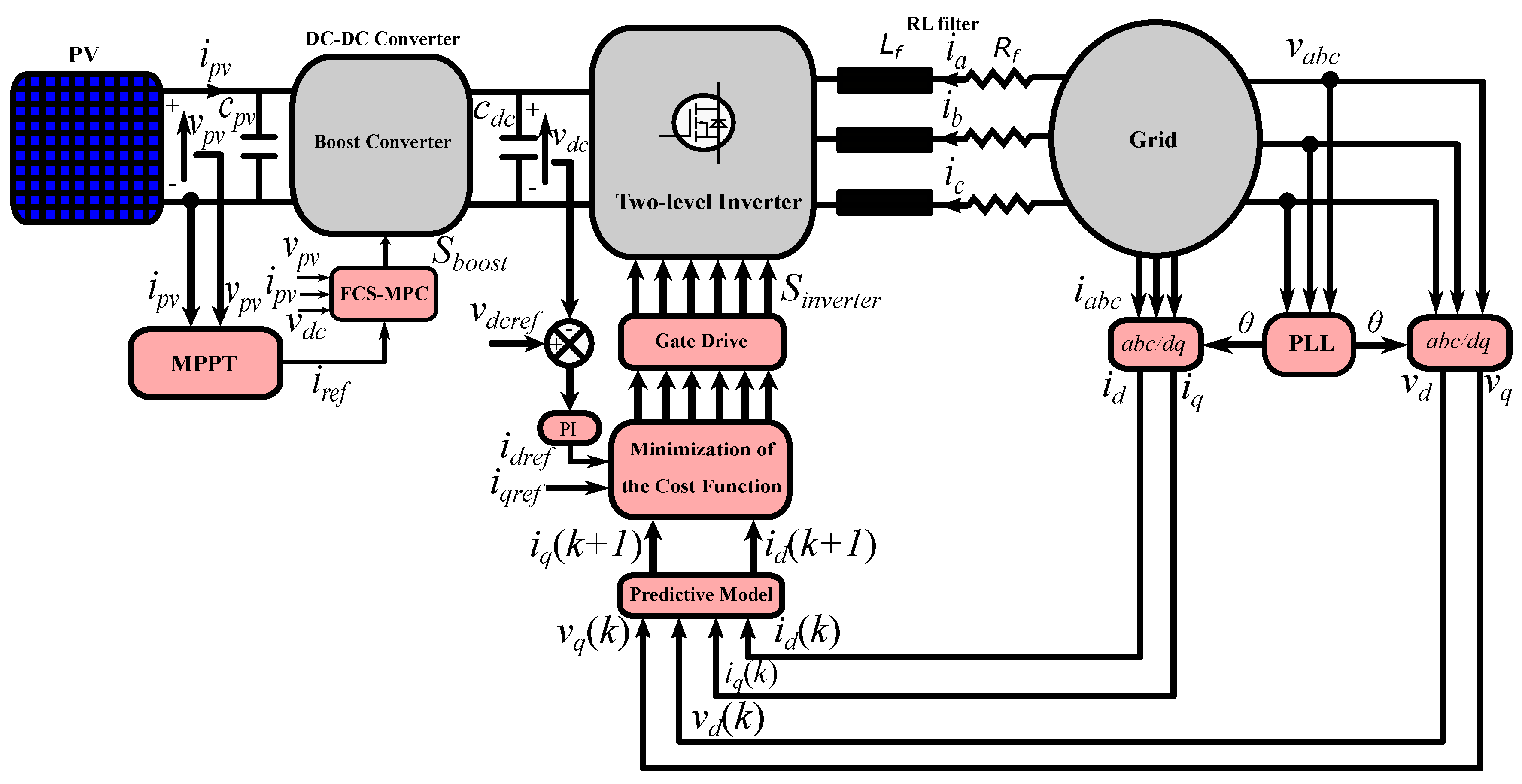
3. Control of the Two-Level Inverter Using FCS-MPC

The PV generated DC energy is fed into the grid and converted to AC energy by means of inverters. In this study, a two-level inverter is utilized; its model and control strategies with the conventional and proposed FCS-MPC will be addressed in the coming subsections.

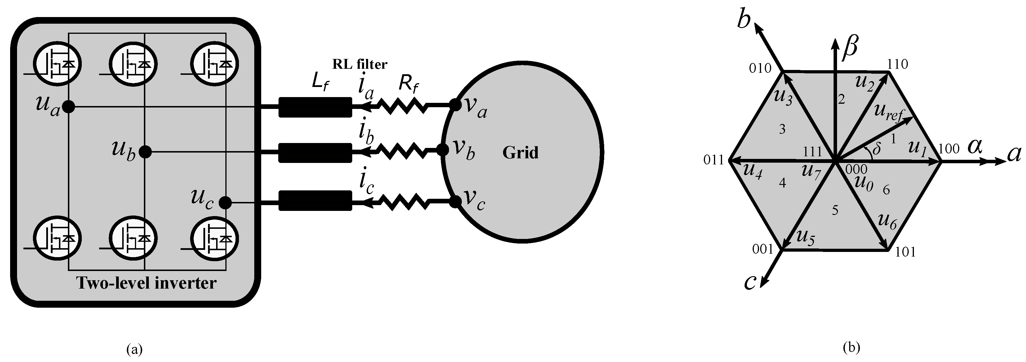
3.1. Two-Level Inverter Model with Grid Connection

Figure 9 shows the configuration of the inverter, filter and the grid. The two-level inverter has eight possible switching actions, shown also in Figure 9 with their sectors distribution (1–6). According to these potential actions, eight voltage vectors can be generated at the output terminals of the inverter.

Table 1. Switching actions and output voltages of the two-level inverter in $\alpha$$\beta$ and $abc$ frames.

Voltage Vectors	Switching States (${\mathit{S}}_{\mathit{abc}}$)	Output Voltages (${\mathit{v}}_{\mathit{\alpha }}$,${\mathit{v}}_{\mathit{\beta }}$)		Output Voltages (${\mathit{v}}_{\mathit{a}}$,${\mathit{v}}_{\mathit{b}}$,${\mathit{v}}_{\mathit{c}}$)
$u_0$	000	0	0	0	0	0
$u_1$	100	$\frac{2v_{dc}}{3}$	0	$\frac{2v_{dc}}{3}$	$\frac{-v_{dc}}{3}$	$\frac{-v_{dc}}{3}$
$u_2$	110	$\frac{v_{dc}}{3}$	$\frac{\sqrt{3}{v}_{dc}}{3}$	$\frac{v_{dc}}{3}$	$\frac{v_{dc}}{3}$	$\frac{-2v_{dc}}{3}$
$u_3$	010	$\frac{-v_{dc}}{3}$	$\frac{\sqrt{3}{v}_{dc}}{3}$	$\frac{-v_{dc}}{3}$	$\frac{2v_{dc}}{3}$	$\frac{-v_{dc}}{3}$
$u_4$	011	$\frac{-2v_{dc}}{3}$	0	$\frac{-2v_{dc}}{3}$	$\frac{v_{dc}}{3}$	$\frac{v_{dc}}{3}$
$u_5$	001	$\frac{-v_{dc}}{3}$	$\frac{-\sqrt{3}{v}_{dc}}{3}$	$\frac{-v_{dc}}{3}$	$\frac{-v_{dc}}{3}$	$\frac{2v_{dc}}{3}$
$u_6$	101	$\frac{v_{dc}}{3}$	$\frac{-\sqrt{3}{v}_{dc}}{3}$	$\frac{v_{dc}}{3}$	$\frac{-2v_{dc}}{3}$	$\frac{v_{dc}}{3}$
$u_7$	111	0	0	0	0	0

summarizes the possible switching actions and output voltage vectors. It is worth mentioning that six active voltage vectors are produced from the inverter with two zero voltage vectors.

Referring to Figure 9 and applying KVL at the inverter output side yields

$$v_x=u_x+L_f\frac{d{i}_x}{dt}+R_f{i}_x,$$

(13)

where x$\in \{a,b,c\}$, $v_x$ are the grid side voltages, $u_x$ are the inverter side voltages, $L_f$ is the filter inductance and $R_f$ is the filter resistance. The output voltages of the inverter is given by [59,60]

$$u_x=\frac{1}{3}{v}_{dc}{T}_x{S}_x,$$

(14)

where $v_{dc}$ is the coupling capacitor voltage; $S_x$ is the switching state vector of the two-level inverter and ∈$\{0,1\}$; and $T_x$ is the coefficient matrix, which can be expressed as

$$T_x=\left[\begin{array}{ccc}2& -1& -1\\ -1& 2& -1\\ -1& -1& 2\end{array}\right].$$

(15)

In the stationary reference frame ($\alpha$-$\beta$), and using Clarke transformation, the inverter voltages are specified as

$$u_{\alpha \beta }=\frac{2}{3}\left[\begin{array}{ccc}1& -\frac{1}{2}& -\frac{1}{2}\\ 0& \frac{\sqrt{3}}{2}& -\frac{\sqrt{3}}{2}\end{array}\right]u_x,$$

(16)

so Equation (13) can be rewritten as

$$v_{\alpha \beta }=u_{\alpha \beta }+L_f\frac{d{i}_{\alpha \beta }}{dt}+R_f{i}_{\alpha \beta }.$$

(17)

Furthermore, and using Park transformation, the rotating reference frame (d-q) components of the voltages can be expressed as

$$\begin{array}{c}{v}_d=u_d+L_f\frac{d{i}_d}{dt}+R_f{i}_d-\omega L_f{i}_q,\hfill \\ v_q=u_q+L_f\frac{d{i}_q}{dt}+R_f{i}_q+\omega L_f{i}_d,\hfill \end{array}$$

(18)

where $\omega$ is the grid frequency. Considering a balanced three phase system, the active and reactive power in different frames are obtained as

$$\begin{array}{c}P=\frac{3}{2}(v_{\alpha }{i}_{\alpha }+v_{\beta }{i}_{\beta }),\hfill \\ Q=\frac{3}{2}(v_{\beta }{i}_{\alpha }-v_{\alpha }{i}_{\beta }),\hfill \end{array}$$

(19)

$$\begin{array}{c}P=\frac{3}{2}(v_d{i}_d+v_q{i}_q),\hfill \\ Q=\frac{3}{2}(v_q{i}_d-v_d{i}_q),\hfill \end{array}$$

(20)

where Equation (19) is in the $\alpha$-$\beta$ frame, while Equation (20) is in the d-q frame.

3.2. Conventional FCS-MPC

To design the FCS-MPC, the discrete time model of the grid-connected inverter (derived earlier) is required. Rearranging Equation (18) gives

$$\begin{array}{c}\frac{d{i}_d}{dt}=-\frac{R_f}{L_f}{i}_d+\omega i_q+\frac{1}{L_f}(v_d-u_d),\hfill \\ \frac{d{i}_q}{dt}=-\frac{R_f}{L_f}{i}_q-\omega i_q+\frac{1}{L_f}(v_q-u_q).\hfill \end{array}$$

(21)

Applying forward Euler method, the following results

$$\begin{array}{c}{i}_d(k+1)=(1-\frac{T_s{R}_f}{L_f})i_d\left(k\right)+\omega T_s{i}_q+\frac{T_s}{L_f}(v_d\left(k\right)-u_d\left(k\right)),\hfill \\ i_q(k+1)=(1-\frac{T_s{R}_f}{L_f})i_q\left(k\right)-\omega T_s{i}_d+\frac{T_s}{L_f}(v_q\left(k\right)-u_q\left(k\right)).\hfill \end{array}$$

(22)

The predicted currents are calculated for the possible switching actions (eight times). Then, the optimal voltage vector is applied to the inverter based on the cost function design as

$$g_i=|i_d{(k+1)}_{u_{0,\dots ,7}}-i_{dref}(k+1)|+|i_q{(k+1)}_{u_{0,\dots ,7}}-i_{qref}(k+1)|,$$

(23)

where $i_{dref}(k+1)$ and $i_{qref}(k+1)$ are the reference currents. The procedure for controlling the grid-connected inverter with conventional FCS-MPC is clarified in Figure 10.

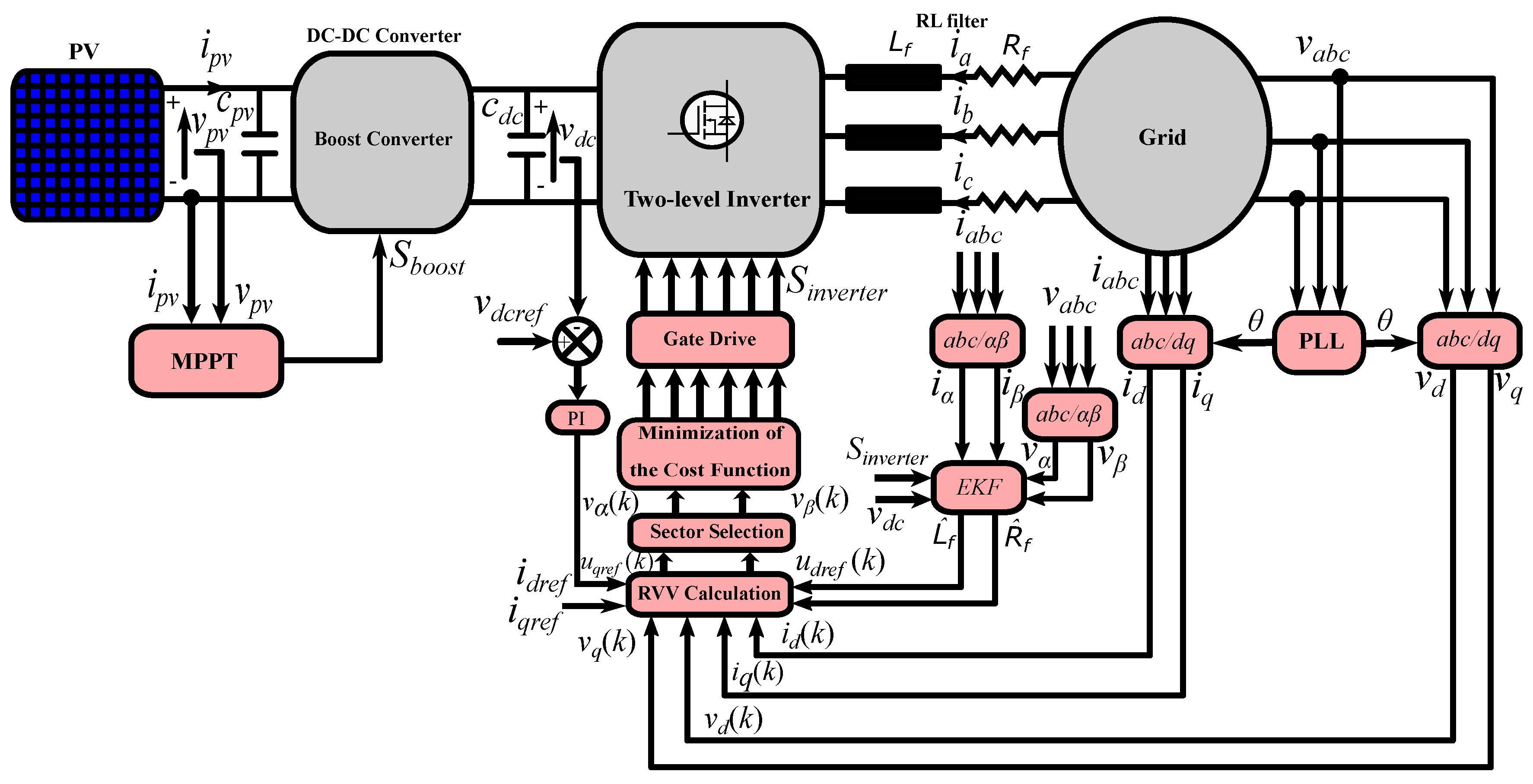
3.3. Proposed FCS-MPC

The conventional FCS-MPC suffers from high calculation burden (seven prediction of current and the cost function is evaluated seven times), so—to decrease the computational effort as well—the reference voltage vector (RVV) is directly calculated in the proposed FCS-MPC. This can be accomplished by substituting $i_{dref}(k+1)$ and $i_{qref}(k+1)$ instead of $i_d(k+1)$ and $i_q(k+1)$ in Equation (22), which results

$$\begin{array}{c}{u}_{dref}\left(k\right)=-{\widehat{R}}_f{i}_d\left(k\right)-\frac{{\widehat{L}}_f}{T_s}(i_{dref}(k+1)-i_d\left(k\right))+\omega {\widehat{L}}_f{i}_q+v_d\left(k\right),\hfill \\ u_{qref}\left(k\right)=-{\widehat{R}}_f{i}_q\left(k\right)-\frac{{\widehat{L}}_f}{T_s}(i_{qref}(k+1)-i_q\left(k\right))-\omega {\widehat{L}}_f{i}_d+v_q\left(k\right),\hfill \end{array}$$

(24)

where ${\widehat{R}}_f$ and ${\widehat{L}}_f$ are the estimated filter parameters. Then, using Park transformation

$$u_{\alpha \beta ref}\left(k\right)=\left[\begin{array}{cc}cos\left(\theta \right)& sin\left(\theta \right)\\ -sin\left(\theta \right)& cos\left(\theta \right)\end{array}\right]u_{dqref}\left(k\right).$$

(25)

As a result, the position (sector) of the reference voltage in the $\alpha$-$\beta$ frame, as shown in Figure 9, can be computed as

$$\delta \left(k\right)=atan2(u_{\beta ref}\left(k\right),u_{\alpha ref}\left(k\right)).$$

(26)

Therefore, the cost function subjected to minimization is modified to

$$g_m=|u_{\alpha }\left(k\right)-u_{\alpha ref}\left(k\right)|+|u_{\beta }\left(k\right)-u_{\beta ref}\left(k\right)|,$$

(27)

where $u_{\alpha }\left(k\right)$ and $u_{\beta }\left(k\right)$ are the voltage vectors in a certain sector and adjacent to the reference voltage vector $\left(u_{ref}\right)$ specified according to Equation (26), as illustrated in Figure 9. According to this design of cost function, and based on sector selection, only three calculations of the cost function are required to get the optimal switching vector. For example, if the selected sector is sector one, the two voltage vectors 100 and 110 along with one of the zeros voltage vectors (000 or 111) are evaluated in the cost function. The modified FCS-MPC scheme is illustrated in Figure 11.

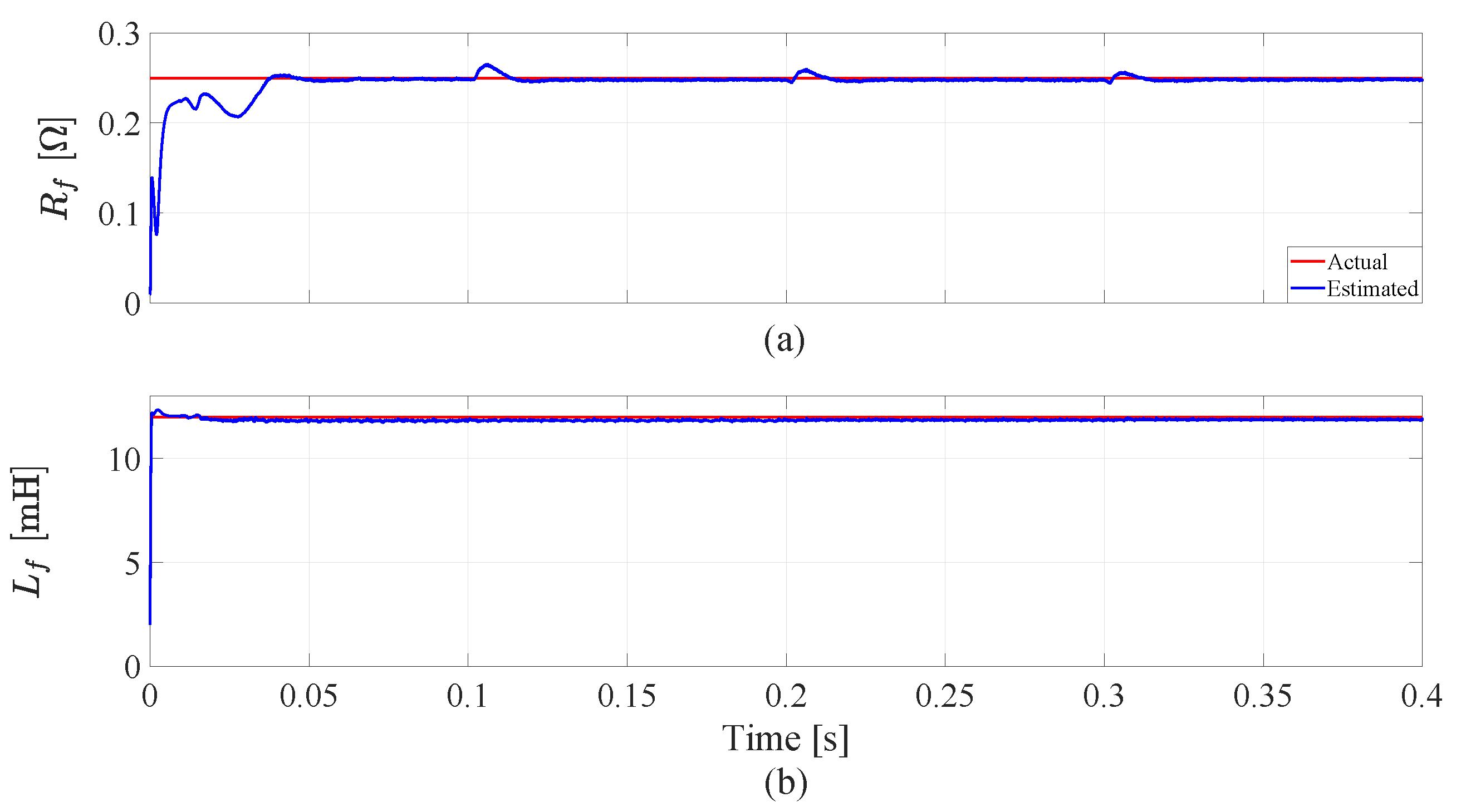
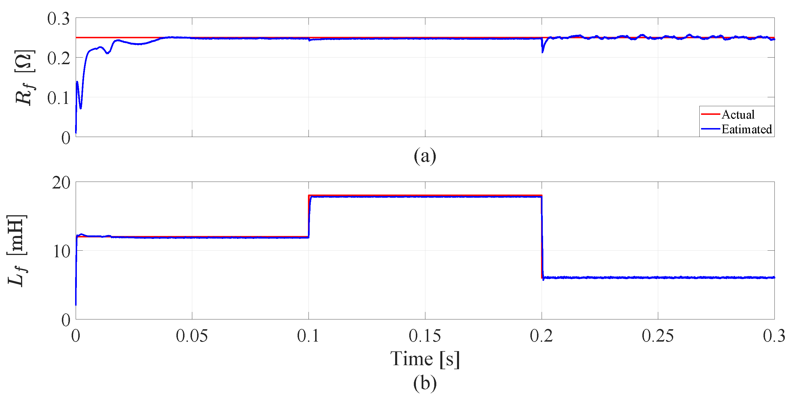
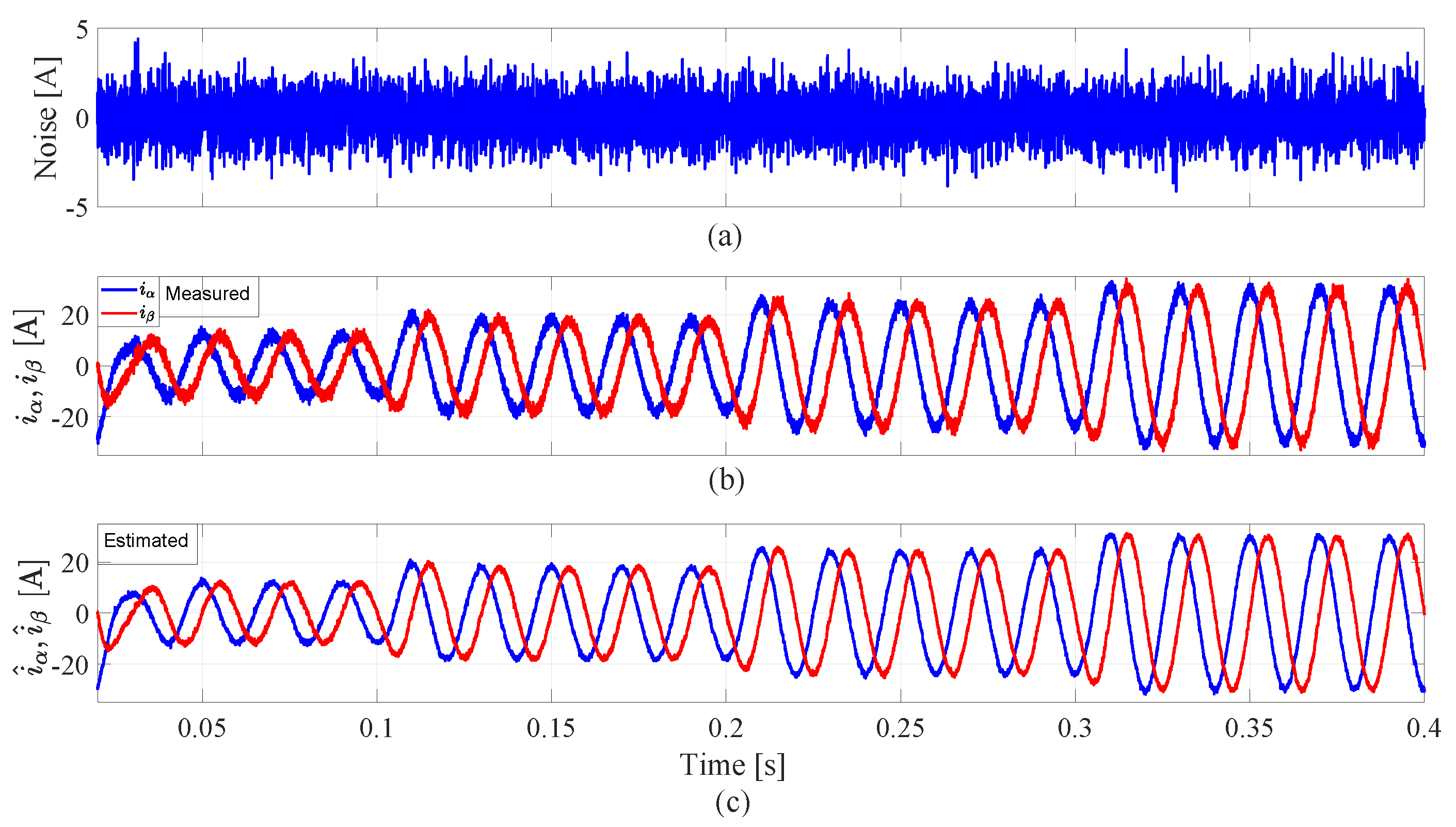
4. Design of the Proposed Extended Kalman Filter

Extended Kalman filter is a powerful tool for states’ and parameters’ estimation. A great advantage of EKF is its filtering capability and noise rejection [61]. It is designed based on the nonlinear discrete-time model of the system [48,61]. Obviously, FCS-MPC depends also on the discrete model of the system, so EKF and FCS-MPC fit very well together. In fact, and as mentioned previously, the FCS-MPC depends on the system parameters. Hence, a major concern is selecting an inaccurate sector and a more incorrect voltage vector, if these parameters are subjected to change. A main contribution of this paper is to eliminate the FCS-MPC dependency on the parameters of the system by estimating the values of the RL filter; i.e., the filter resistance and inductance by means of EKF. In reality, the filter parameters are exposed to variation due to aging, heat or saturation.

To implement the EKF, the discrete time nonlinear state space model of the grid connected inverter can be derived by rearranging Equation (17) as

$$\frac{d{i}_{\alpha \beta }}{dt}=-\frac{R_f}{L_f}{i}_{\alpha \beta }+\frac{1}{L_f}(v_{\alpha \beta }-u_{\alpha \beta }).$$

(28)

Thus, the model of the grid-connected inverter including disturbance can be written as

$$\begin{array}{c}\dot{x}=\mathbf{A}x+\mathbf{B}u+w,\hfill \\ y=\mathbf{C}x+\mathbf{D}u+v,\hfill \end{array}$$

(29)

where x = [$i_{\alpha }$ $i_{\beta }$ $R_f$ $L_f$ ]${}^T$ is the state vector, u = [($v_{\alpha }$-$u_{\alpha }$) ($v_{\beta }$-$u_{\beta }$)]${}^T$ is the input, y = [$i_{\alpha }$ $i_{\beta }$ ]${}^T$ is the measurement, w is the system uncertainty with covariance matrix $\mathbf{Q}$ and v is the measurement noise with covariance matrix $\mathbf{R}$. Further, $\mathbf{A}$, $\mathbf{B}$, $\mathbf{C}$ and $\mathbf{D}$ are the inverter system matrices, and based on Equation (28) they are defined as

$$\mathbf{A}=\left[\begin{array}{cccc}-\frac{R_f}{L_f}& 0& 0& 0\\ -\frac{R_f}{L_f}& 0& 0& 0\\ 0& 0& 0& 0\\ 0& 0& 0& 0\end{array}\right],\mathbf{B}=\left[\begin{array}{c}\frac{1}{L_f}\\ \frac{1}{L_f}\\ 0\\ 0\end{array}\right],\mathbf{C}=\left[\begin{array}{cccc}1& 0& 0& 0\\ 0& 1& 0& 0\end{array}\right],\mathbf{D}=0.$$

(30)

Hence, the discrete model can be expressed as

$$\begin{array}{c}x(k+1)={\mathbf{A}}_{d}x\left(k\right)+{\mathbf{B}}_{d}u\left(k\right)+w\left(k\right),\hfill \\ y\left(k\right)={\mathbf{C}}_{d}x\left(k\right)+{\mathbf{D}}_{d}u\left(k\right)+v\left(k\right),\hfill \end{array}$$

(31)

where ${\mathbf{A}}_d=\mathbf{I}+\mathbf{A}{T}_s$, ${\mathbf{B}}_d=\mathbf{B}{T}_s$, ${\mathbf{C}}_d=\mathbf{C}$, ${\mathbf{D}}_d=\mathbf{D}$ and $\mathbf{I}$ is the identity matrix. Normally, the system uncertainty and measurement noise are not known, so the EKF is implemented as follows:

$$\begin{array}{c}\widehat{x}(k+1)={\mathbf{A}}_d\widehat{x}\left(k\right)+{\mathbf{B}}_{d}u\left(k\right)+\mathbf{K}\left(k\right)(y\left(k\right)-\widehat{y}\left(k\right)),\hfill \\ \widehat{y}\left(k\right)={\mathbf{C}}_d\widehat{x}\left(k\right)+{\mathbf{D}}_{d}u\left(k\right),\hfill \end{array}$$

(32)

where $\mathbf{K}\left(k\right)$ is the Kalman gain, $\widehat{x}\left(k\right)$ and $\widehat{y}\left(k\right)$ are the estimated quantities. Finally, the Kalman filter can be implemented through two stages of prediction and correction, following this procedure:

• Initialize the state vector and covariance matrices.
• Prediction of state vector

  $${\widehat{x}}^{-}\left(k\right)={\mathbf{A}}_d\widehat{x}(k-1)+{\mathbf{B}}_{d}u(k-1).$$

  (33)
• Error covariance matrix prediction

  $${\mathbf{P}}^{-}\left(k\right)=f\left(k\right)\mathbf{P}(k-1)f{\left(k\right)}^{\mathrm{T}}+\mathbf{Q},$$

  (34)

  where

  $$f\left(k\right)=\frac{\partial }{\partial x}({\mathbf{A}}_{d}x\left(k\right)+{\mathbf{B}}_{d}u\left(k\right)){|}_{{\widehat{x}}^{-}\left(k\right)}.$$

  (35)

  Kalman gain calculation

  $$\mathbf{K}\left(k\right)={\mathbf{P}}^{-}\left(k\right){\mathbf{C}}_d^{\mathrm{T}}{({\mathbf{C}}_d{\mathbf{P}}^{-}\left(k\right){\mathbf{C}}_d^{\mathrm{T}}+\mathbf{R})}^{-1}.$$

  (36)
• Estimation update through measurements

  $$\widehat{x}\left(k\right)={\widehat{x}}^{-}\left(k\right)+\mathbf{K}\left(k\right)(y\left(k\right)-{\mathbf{C}}_d\widehat{x}-\left(k\right)).$$

  (37)
• Error covariance matrix update

  $$\mathbf{P}\left(k\right)={\mathbf{P}}^{-}\left(k\right)-\mathbf{K}\left(k\right){\mathbf{C}}_d{\mathbf{P}}^{-}\left(k\right).$$

  (38)
• Go back to step 2.

5. Simulation Results and Discussion

The proposed PV system is shown in Figure 11. It consists of a PV array of $15$ kW (15 series × 5 parallel), followed by a boost converter, where the MPPT function is accomplished by FCS-MPC and the direct switching technique. The FCS-MPC generates the switching state for the boost converter to follow the reference current coming from outer-side loop developed by the P&O technique. The switching state (0 or 1) identified by the cost function (g) will be enforced to the power switch in the boost circuit. In the proposed MPPT, the switching state is generated directly. Then, the extracted power from the PV source is fed to the two-level inverter. The two-level inverter has two control loops for the purpose of active and reactive power control. The first and outer loop is achieved by PI controller to stabilize the DC-link capacitor voltage at its reference value ($v_{dcref}$) and to provide the reference current ($i_{dref}$) to the inner loop, where $i_{qref}$ is set to zero for unity power factor operation. In this study, the inner current loop is realized by the conventional and the proposed FCS-MPC technique. In the conventional one, the predicted currents is calculated and then the voltage vector (out of seven) corresponding to the minimum cost function ($g_i$) will be selected. It is obvious that to get this optimal vector, 14 iterations (seven for the currents, and seven for the cost function) are required in the inner loop. This in turn increases the computational burden. However, in the proposed FCS-MPC technique, the RVV is computed to narrow the calculation range from six sectors to only one sector. This greatly reduces the computation time as only three computations of the cost function ($g_m$) are required in the specified sector. Furthermore, and to avoid the potential variation in the parameters of the grid connected inverter, an EKF is employed to estimate and correct these values online. The parameters of the PV grid connected system are summed up in

Table 2. PV grid-connected system parameters.

Parameter	Value
PV array power [kW]	15
Boost inductance $L_b$ [$\mathrm{m}\mathrm{H}$]	25
DC-link capacitance $c_{dc}$ [$\mathsf{\mu }\mathrm{F}$]	1000
Filter inductance $L_f$ [$\mathrm{m}\mathrm{H}$]	12
Filter resistance $R_f$ [$\Omega$]	$0.25$
DC-link reference voltage $v_{dcref}$ [$\mathrm{V}$]	700
Grid frequency $\omega$ [$\mathrm{rad}/\mathrm{s}$]	$2\pi \times 50$
Grid line-line voltage v [$\mathrm{V}$]	400
Sampling time $T_s$ [$\mathsf{\mu }\mathrm{s}$]	40

.

The simulation results are divided to two subsections under different atmospheric conditions and parameter variations, where the performance of the proposed scheme is compared with the conventional FCS-MPC as follows:

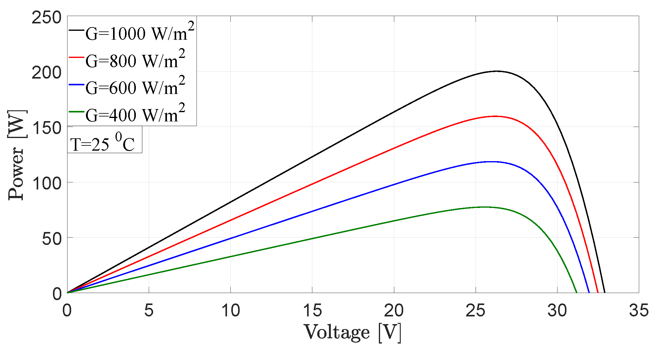
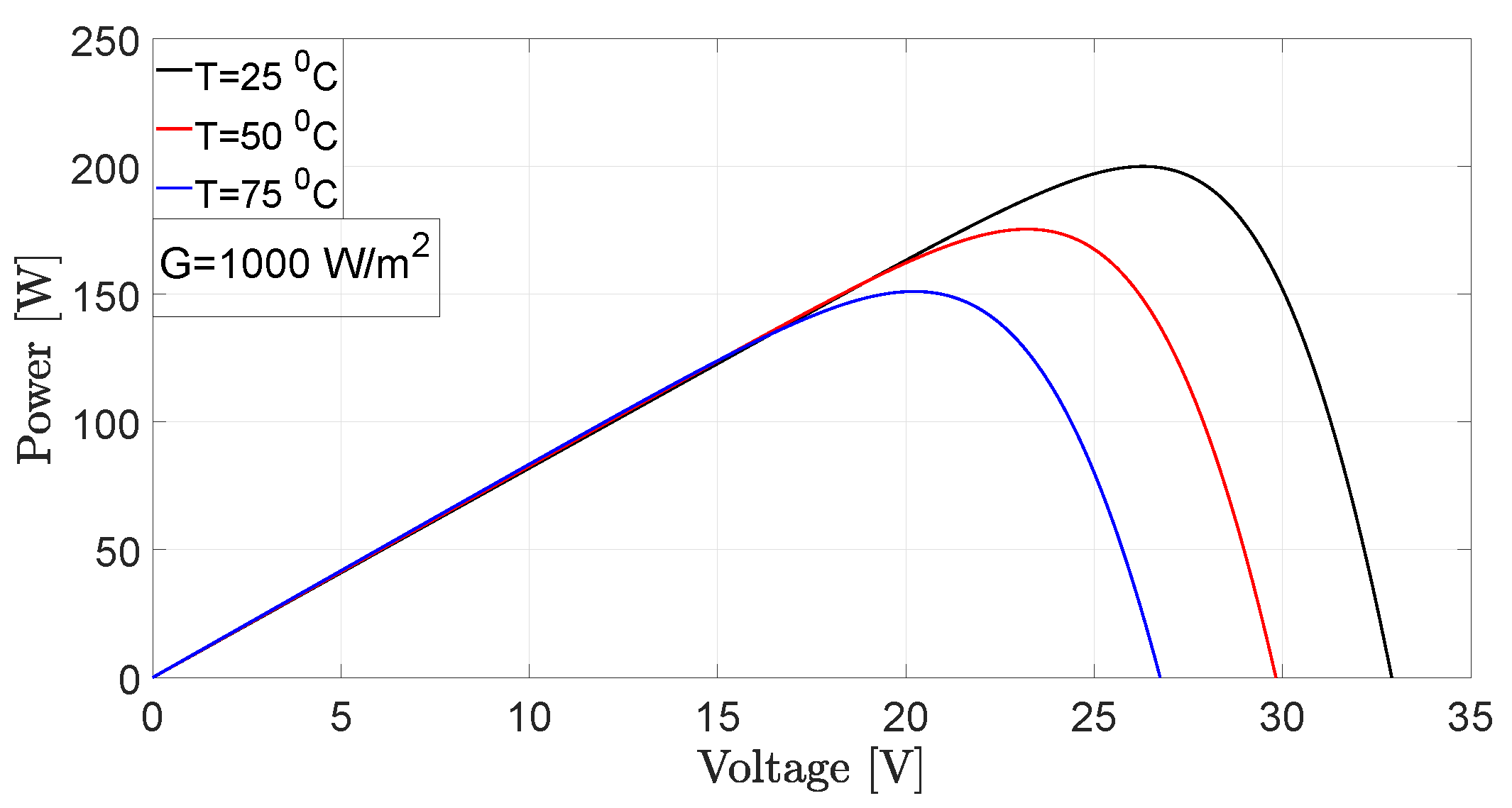
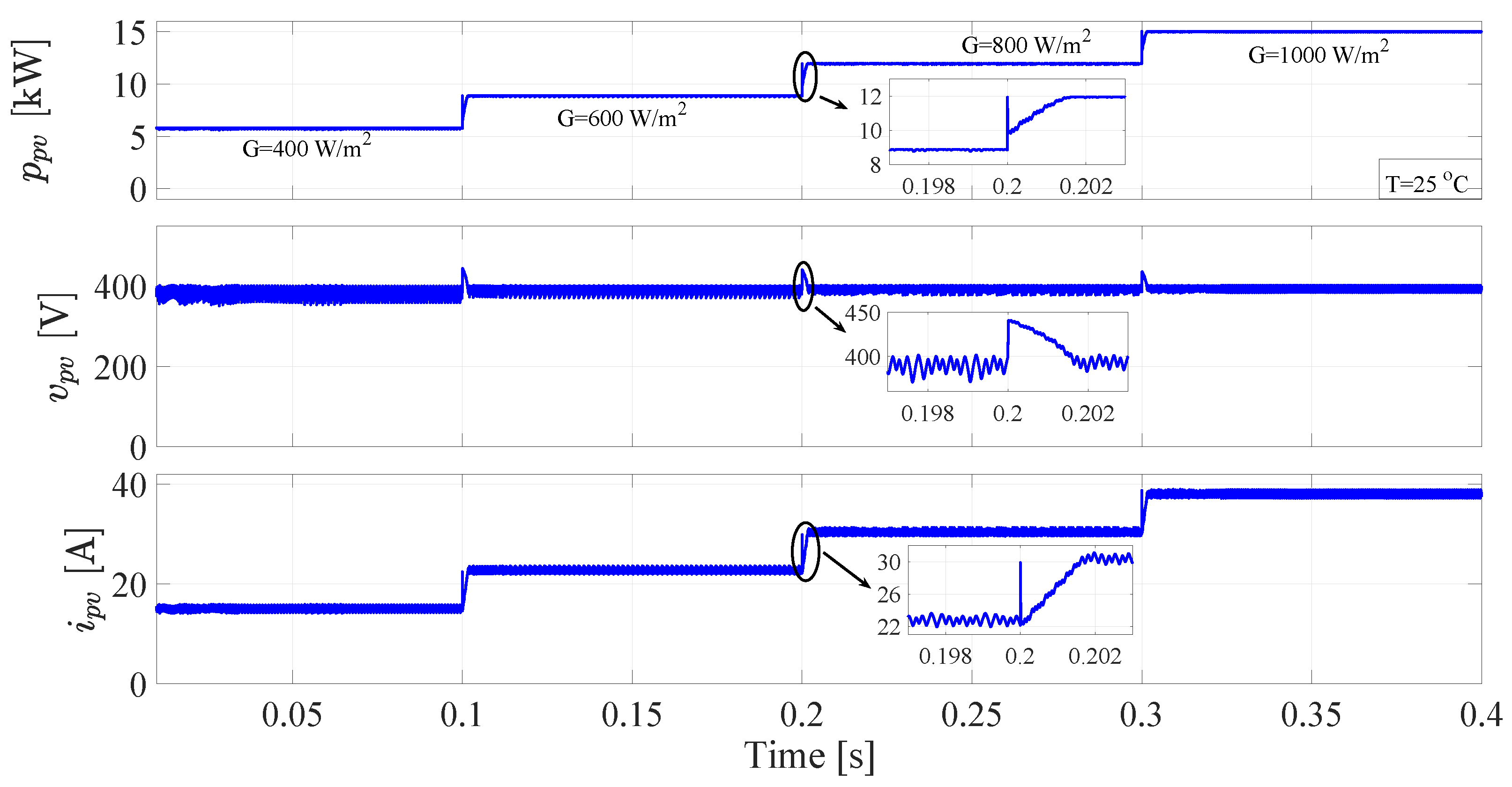
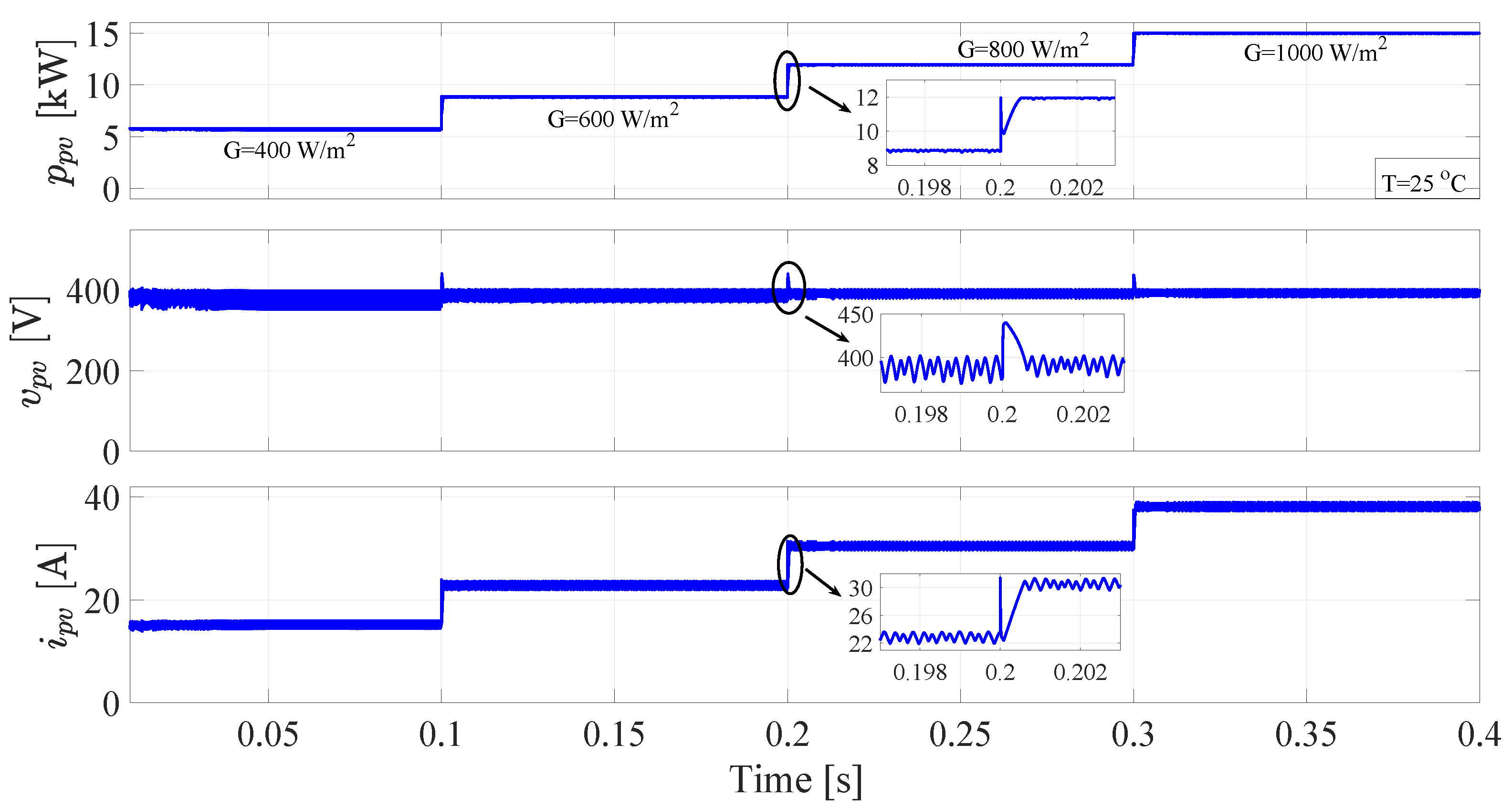
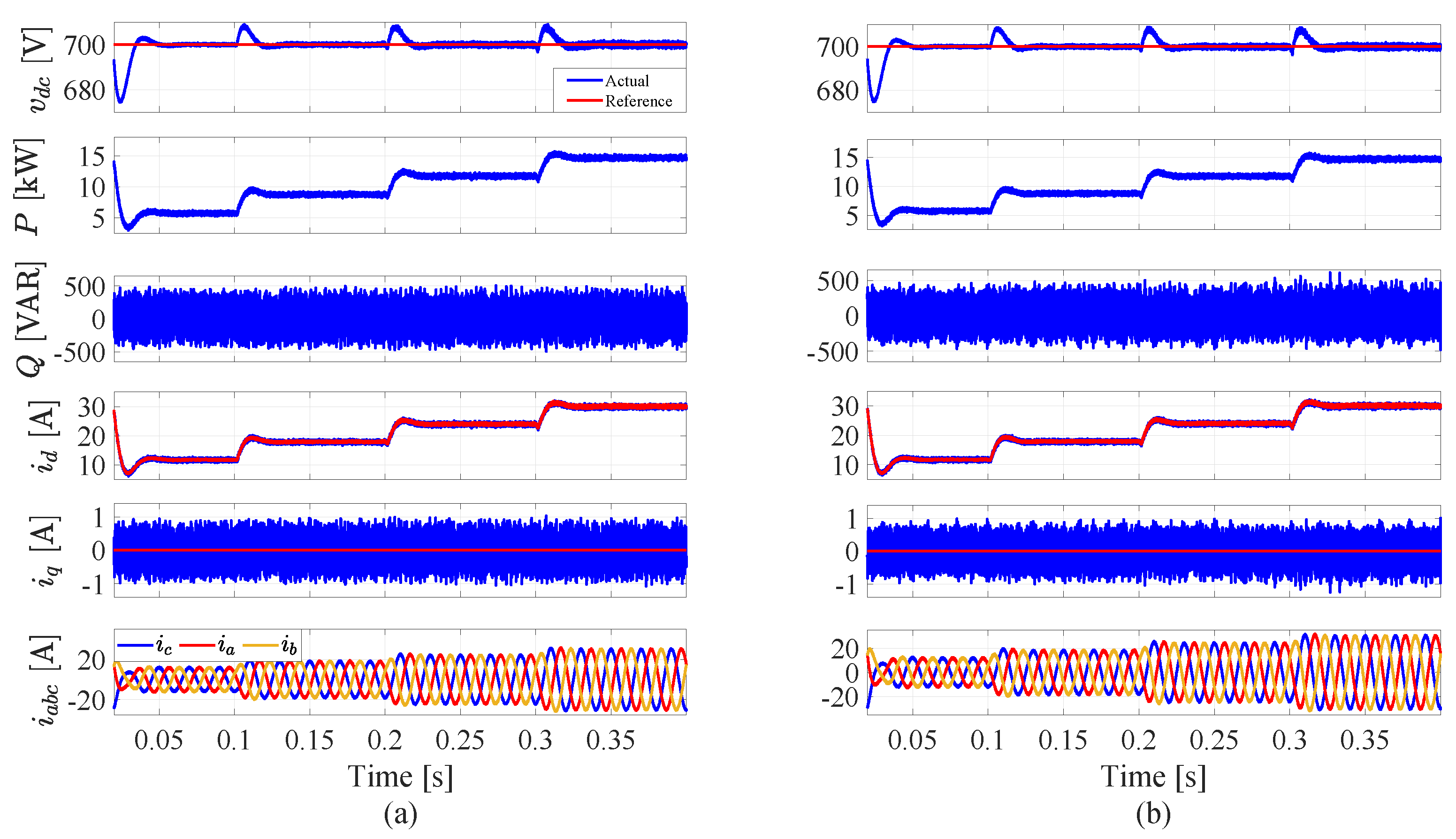
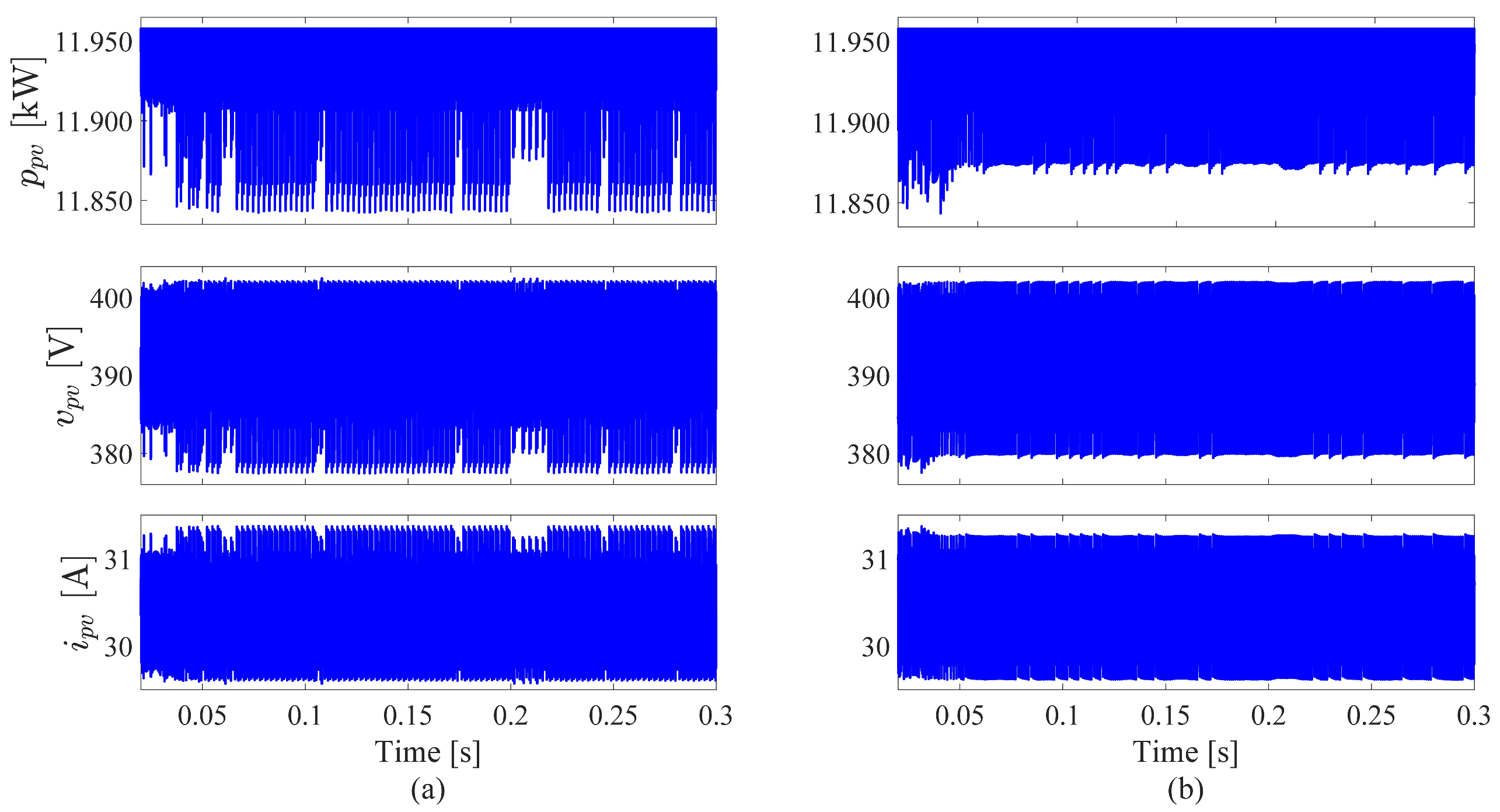
5.1. MPPT and System Behavior under Different Radiation Conditions

Figure 12 and Figure 13 show the behavior of the proposed MPPT and the conventional one. The results are performed at different radiation conditions ranging from $400\mathrm{W}/{\mathrm{m}}^2$ to $1000\mathrm{W}/{\mathrm{m}}^2$. It is clear that the proposed MPPT has a very fast transient behavior in comparison with the conventional FCS-MPC. As there is no need for current prediction computation in the proposed algorithm, the calculation time is highly reduced. The tracking speed of the proposed direct switching method is $0.5$ $\mathrm{m}\mathrm{s}$, while it is $1.6$ $\mathrm{m}\mathrm{s}$ for the conventional MPPT. Besides, the average switching frequency for the direct switching technique is $4.42$ kHz, while the conventional technique has a higher average switching frequency of $4.85$ kHz.

The performance of the inverter control using the conventional and the proposed FCS-MPC with EKF is investigated at the previous radiation conditions, and shown in Figure 14, where the DC-link voltage ($v_{dc}$), the active power injected into the gird (P), reactive power (Q), the direct axis current ($i_d$), the quadrature axis current ($i_q$) and the $abc$ currents are illustrated respectively. The DC-link voltage tracks its reference value with a very low overshoot of $1.5$% for both of the conventional and the proposed techniques. The active power behavior is similar in the two methods. However, the reactive power has a lower ripple content in the proposed strategy due to the enhanced tracking of $i_q$, as clarified in Figure 15.

Furthermore, the total harmonic distortion (THD) of the proposed approach is better than the conventional one, despite of the lower average switching frequency of the proposed FCS-MPC. A comparative summary is provided in

Table 3. Performance summaries of the conventional and the proposed FCS-MPC.

Condition	THD		Average Switching Frequency
	Conventional	Proposed	Conventional	Proposed
$400[\mathrm{W}/{\mathrm{m}}^2]$	4.24%	3.87%
$600[\mathrm{W}/{\mathrm{m}}^2]$	2.80%	2.58%	3.99 kHz	3.81 kHz
$800[\mathrm{W}/{\mathrm{m}}^2]$	2.14%	2.04%	for all conditions
$1000[\mathrm{W}/{\mathrm{m}}^2]$	1.74%	1.68%

. Another merit of the proposed technique with EKF is eliminating the prior need of knowledge of the system parameters. Figure 16 shows the estimated filter parameters for the same previous atmospheric conditions. The EKF provides a very fast and accurate online monitoring for the filter inductance ($L_f$) with a maximum error of $1.7$%. However, the filter resistance ($R_f$) estimation is relatively slower than the inductance estimation at the beginning of the simulation, but the estimation is very precise with a maximum error of $0.8$%.

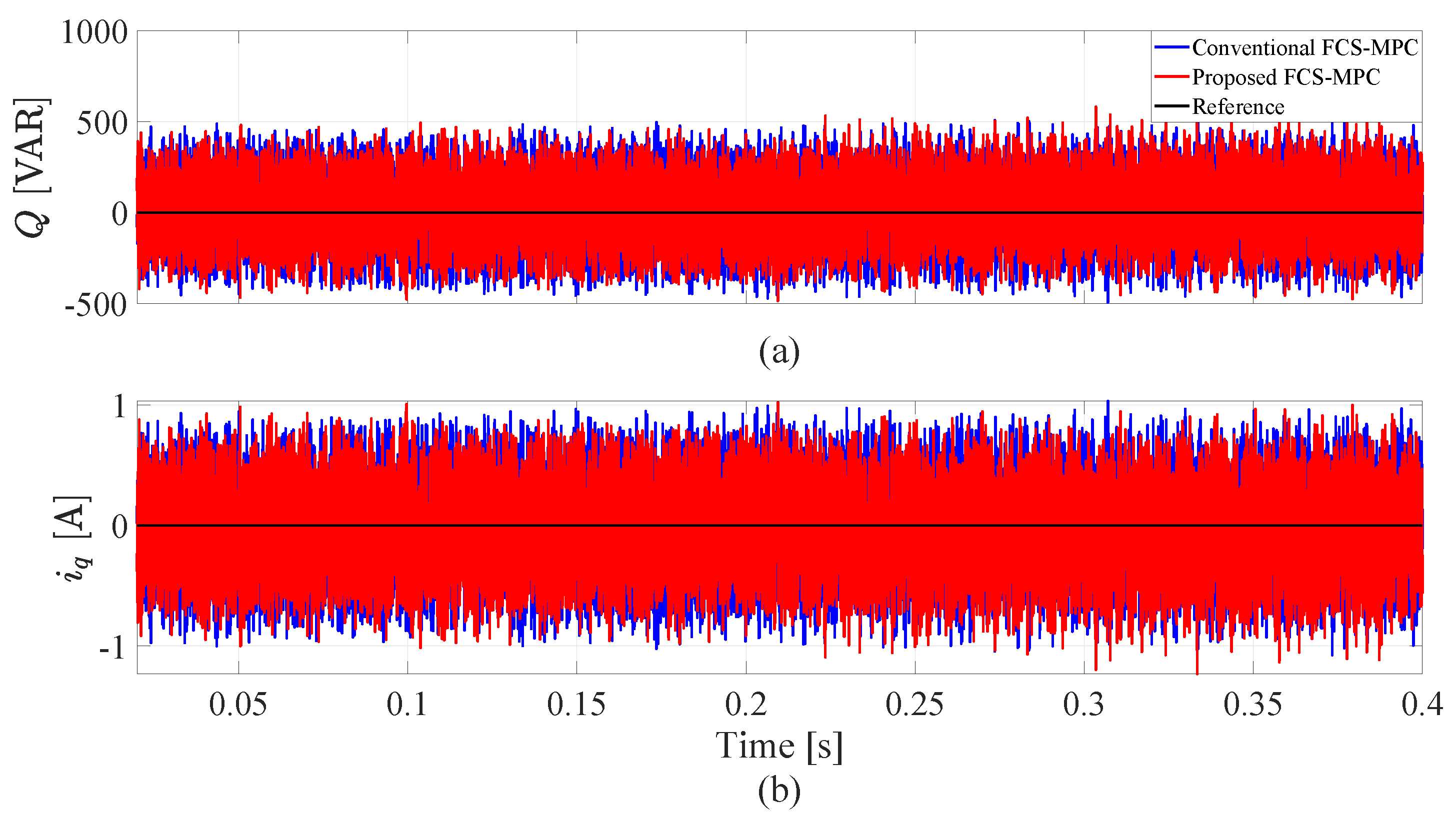
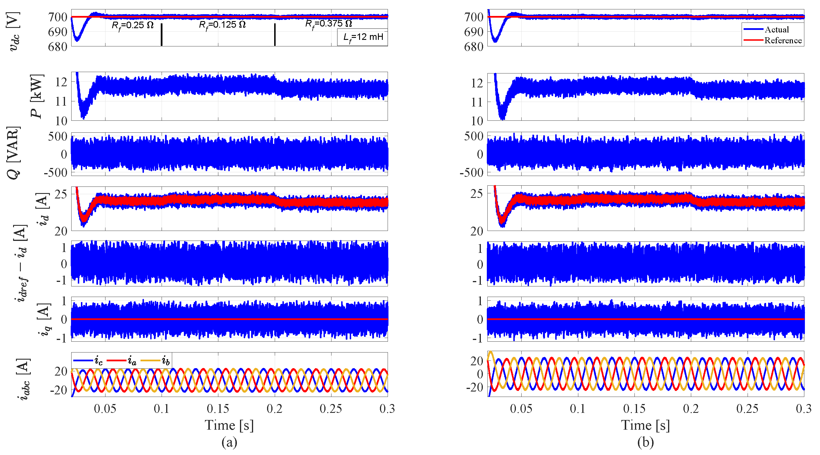
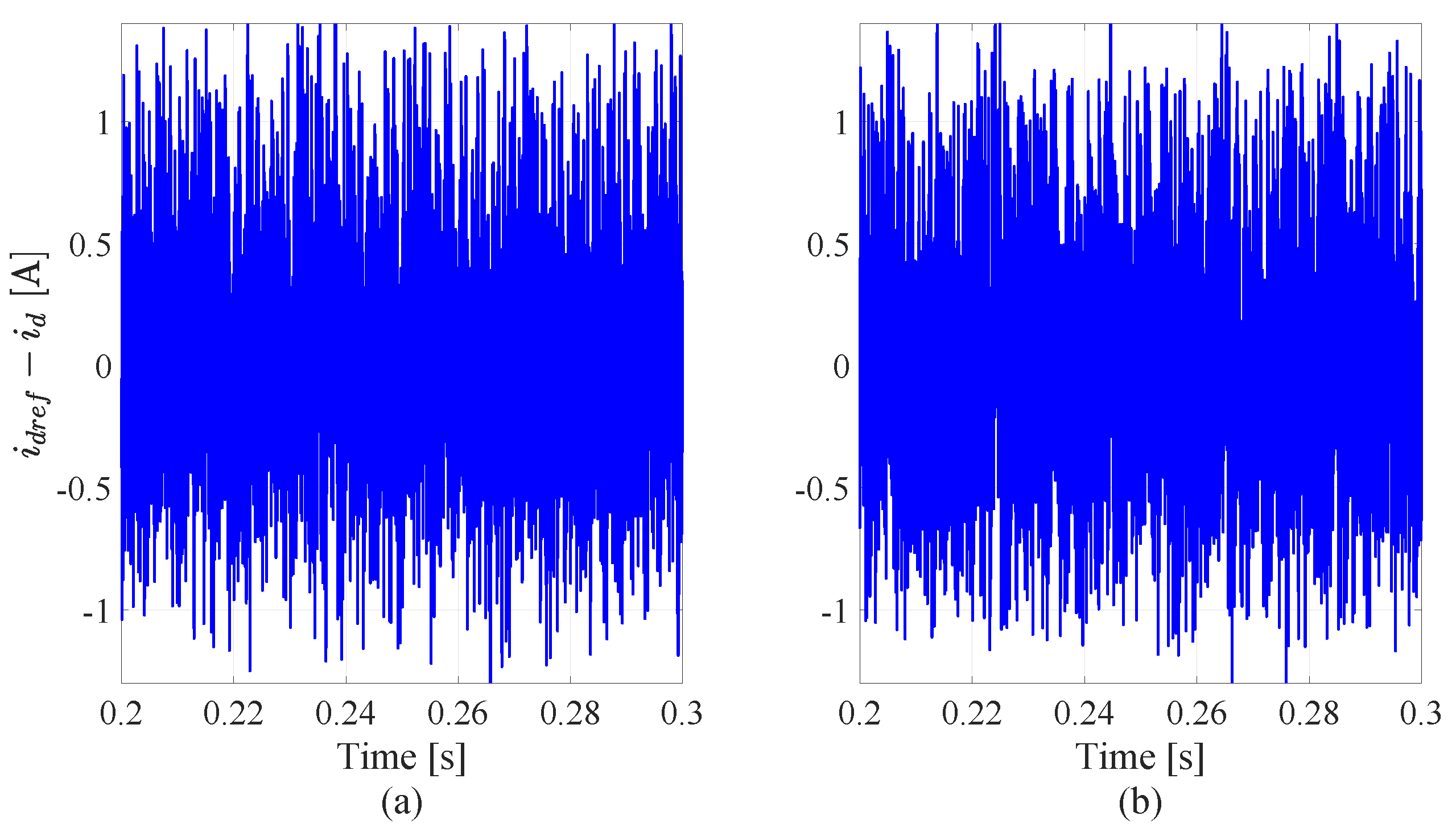
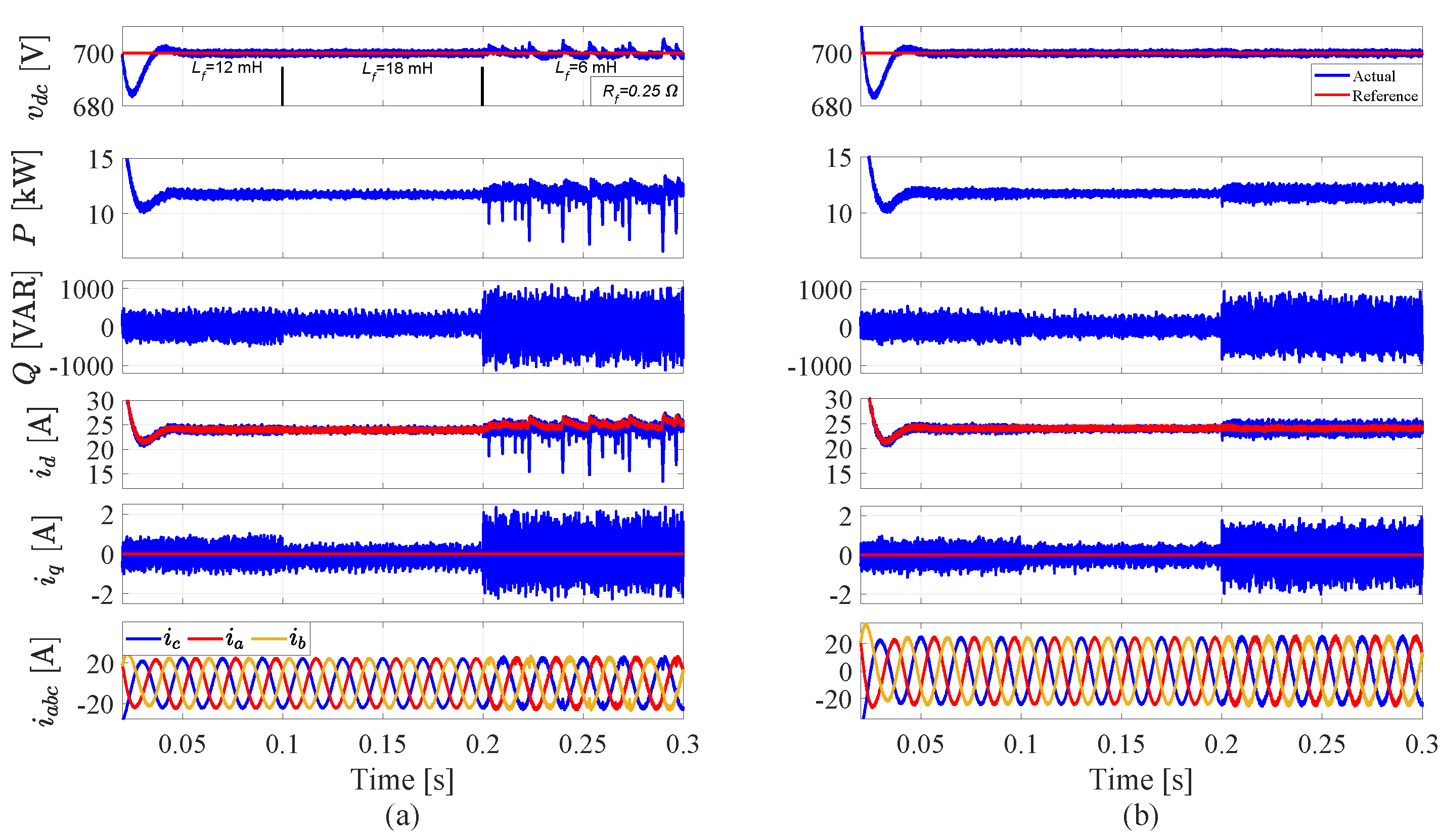
5.2. System Performance with Parameter Variations

In this subsection, the effects of parameter variations on the conventional and the proposed FCS-MPC are investigated. The atmospheric conditions for this test are kept constant at 800 W/m${}^2$ and $25{}^{°}\mathrm{C}$. Figure 17 shows the PV power, voltage and current, respectively. The results of the conventional FCS-MPC MPPT exhibit higher ripples compared with the proposed MPPT in all the waveforms, where the proposed MPPT shows an increased average power extraction, and hence higher energy gain.

Table 4. Energy calculation for the conventional and the proposed MPPT within a one day span (10 h).

Condition	Energy [kWh]		Saving [kWh]
	Conventional	Proposed
800 [W/m${}^2$]	11.9395 × 60 × 60 × 10/0.3	11.9414 × 60 × 60 × 10/0.3	228

presents the energy calculation for the two MPPT techniques within a one day (10 h) period. The difference (saving) between the two methods is about 228 kWh; this amount is calculated through the simulation interval (0.3 s).

Figure 18 illustrates the DC-link voltage, the active power injected into the gird, reactive power, the d-axis current, the difference between the actual d-axis current and its reference value, the q-axis current and the $abc$ currents at different step changes of the filter resistance, respectively. In the first interval, the filter resistance is kept constant at its nominal value $R_f=0.25$ $\Omega$; after that the resistance is decreased to the half of its nominal value i.e., $\Delta R_f=-50\%$, finally it is increased by $+50\%$. Filter resistance change affects the steady state error between $i_d$ and $i_{dref}$, which is obvious at the last interval (0.2–0.3 $\mathrm{s}$) of $i_d$, where $i_d$ is deviated from its reference, unlike the proposed method. This error is further examined in Figure 19 for better observation. However, the effect of resistance change on the THD of the currents is small. Moreover, the estimated values of the filter resistance and inductance are presented in Figure 20, where the EKF provides a very efficient estimation for both of them.

Figure 21 shows the DC-link voltage, the active power injected into the gird, reactive power, the d-axis current, the q-axis current and the $abc$ currents at different step changes of the filter inductance, where the inductance is changed with a mismatch of $\pm 50\%$, respectively. As a matter of fact, it is not strange that the performances of the conventional and the proposed FCS-MPC are enhanced with $+50\%$ mismatch in the filter inductance, as shown in the second interval (0.1–0.2 $\mathrm{s}$); this due to the filtering capability of the inductor. However, this increase affects the steady state error of $i_q$ in the same interval, as shown in Figure 22, and hence the steady state error of the reactive power. Referring to Figure 22, it was found that the steady state error of the conventional FCS-MPC is about 75 (VAR), which is approximately three times the steady state error of the proposed FCS-MPC with 25 (VAR). Underestimating the filter inductance (the third interval) deteriorates the behavior of the conventional FCS-MPC, where the $abc$ currents is greatly distorted. Furthermore, the injected active power exhibits very high ripples. In contrast, the proposed technique with EKF sustains a very good performance with reasonable active power ripples. Thanks to the accurate estimation provided by the EKF as revealed in Figure 23. Furthermore,

Table 5. Total harmonic distortion (THD) of the conventional and the proposed FCS-MPC with filter inductance variation.

Condition	THD
	Conventional	Proposed
12 [$\mathrm{m}\mathrm{H}$]	2.17%	2.07%
18 [$\mathrm{m}\mathrm{H}$]	1.55%	1.47%
6 [$\mathrm{m}\mathrm{H}$]	8.75%	3.69%

gives a comparative evaluation of the two techniques concerning the THD, where the proposed methodology has superior performance, especially when the inductance is underestimated (6 $\mathrm{m}\mathrm{H}$). The difference between the THD of the two techniques with this condition is approximately $5\%$, where the conventional FCS-MPC exceeds the IEEE standards [62].

The EKF is not only parameter estimation tool; it also has a filtering capability. To prove that, a current noise shown in Figure 24 is added to the $\alpha$$\beta$ currents. The estimated currents exhibit a very good refined waveform in comparison with the noisy currents, as revealed in Figure 24.

6. Conclusions

A two-stage, grid-connected PV system is proposed in this paper, wherein the model of each component in the system is examined. The maximum power is extracted from the PV source by a new direct-switching MPPT technique. The proposed technique is very fast as there is no need for a PI controller or a modulation stage. For investigation, the methodology is compared with the conventional FCS-MPC algorithm. The cost function of the conventional MPPT is designed to minimize the error between the reference and the one-step in the horizon-predicted current. The inverter is controlled by a computationally-efficient FCS-MPC technique supported by an EKF to estimate the filter parameters. The proposed methodology determines the sector of the RVV directly from demanded currents, so the cost function is evaluated only three times in the identified sector. The proposed system was compared with the conventional FCS-MPC under different operating conditions of radiation and parameter variation, and validated using Matlab. The results show that the proposed MPPT gives better dynamic and steady state responses than the conventional MPPT with FCS-MPC. Moreover, the results of the proposed MPPT provide enhanced energy utilization in comparison with the conventional MPPT at steady state. Besides, and due to the very high transient behavior of the proposed MPPT, this gain will be higher in large PV arrays (i.e., 1 MW or higher). Furthermore, the results show that the filter inductance has a greater effect on the system’s performance than the filter resistance, especially when considering the THD of the currents. Low inductance values of the filter deteriorate the conventional FCS-MPC behavior. However, the proposed technique offers robust performance, where the EKF presents a delicate estimation for the filter resistance and inductance. This improves the system’s behavior against parameter uncertainties, even preserving the stability of the system. Additionally, the EKF rejects potential noise in the measurements (currents).

References

1. Lee, B.; Liu, J.Z.; Sun, B.; Shen, C.Y.; Dai, G.C. Thermally conductive and electrically insulating EVA composite encapsulants for solar photovoltaic (PV) cell. eXPRESS Polym. Lett. 2008, 2, 357–363. [Google Scholar] [CrossRef]
2. Khalil, A.; Rajab, Z.; Asheib, A. Modeling Simulation Analysis and Control of Stand-alone PV System. In Proceedings of the 7th International Renewable Energy Congress IREC 2016, Hammamet, Tunisia, 22–24 March 2016; pp. 1–6. [Google Scholar]
3. Mohamed, A.; de Cossio, C.F.; Ma, T.; Farhadi, M.; Mohammed, O. Operation and protection of photovoltaic systems in hybrid AC/DC smart grids. In Proceedings of the IECON 2012—38th Annual Conference on IEEE Industrial Electronics Society, Montreal, QC, Canada, 25–28 October 2012; pp. 1104–1109. [Google Scholar]
4. Lekhchine, S.; Bahi, T.; Abadlia, I.; Bouzeria, H. PV-battery energy storage system operating of asynchronous motor driven by using fuzzy sliding mode control. Int. J. Hydrogen Energy 2017, 42, 8756–8764. [Google Scholar] [CrossRef]
5. Elgendy, M.A.; Zahawi, B.; Atkinson, D.J. Comparison of directly connected and constant voltage controlled photovoltaic pumping systems. IEEE Trans. Sustain. Energy 2010, 1, 184–192. [Google Scholar] [CrossRef]
6. Li, C.-H.; Zhu, X.J.; Cao, G.-Y.; Sui, S.; Hu, M.-R. Dynamic modeling and sizing optimization of stand-alone photovoltaic power systems using hybrid energy storage technology. Renew. Energy 2009, 34, 815–826. [Google Scholar] [CrossRef]
7. Vordos, N.; Bandekas, D.; Nolan, J.; Fantidis, J.; Ioannou, A. Design and simulation of hybrid power system with wind turbines, photovoltaics and fuel cells. In Recent Advances in Energy, Environment and Development; WSEAS Press: Rhodes Island, Greece, 16–19 July 2013; pp. 19–24. [Google Scholar]
8. Alajmi, B.N.; Ahmed, K.H.; Adam, G.P.; Williams, B.W. Single-phase single-stage transformer less grid-connected PV system. IEEE Trans. Power Electron. 2012, 28, 2664–2676. [Google Scholar] [CrossRef]
9. Shayestegan, M. Overview of grid-connected two-stage transformer-less inverter design. J. Mod. Power Syst. Clean Energy 2018, 6, 642–655. [Google Scholar] [CrossRef] [Green Version]
10. Das, P.P.; Chattopadhyay, S. A voltage-independent islanding detection method and low-voltage ride through of a two-stage PV inverter. IEEE Trans. Ind. Appl. 2018, 54, 2773–2783. [Google Scholar] [CrossRef]
11. Jahanbakhshi, M.-H.; Asaei, B.; Farhangi, B. A novel deadbeat controller for single phase PV grid connected inverters. In Proceedings of the 2015 23rd Iranian Conference on Electrical Engineering, Tehran, Iran, 10–14 May 2015; pp. 1613–1617. [Google Scholar]
12. Lakshmi, M.; Hemamalini, S. Coordinated control of MPPT and voltage regulation using single-stage high gain DC DC converter in a grid-connected PV system. Electr. Power Syst. Res. 2019, 69, 65–73. [Google Scholar] [CrossRef]
13. Ahmed, M.E.; Orabi, M.; AbdelRahim, O.M. Two-stage micro-grid inverter with high-voltage gain for photovoltaic applications. IET Power Electron. 2013, 6, 1812–1821. [Google Scholar] [CrossRef]
14. Sangwongwanich, A.; Yang, Y.; Blaabjerg, F. High-performance constant power generation in grid-connected PV systems. IEEE Trans. Power Electron. 2015, 31, 1822–1825. [Google Scholar] [CrossRef] [Green Version]
15. Yau, H.-T.; Wu, C.-H. Comparison of extremum-seeking control techniques for maximum power point tracking in photovoltaic systems. Energies 2011, 4, 2180–2195. [Google Scholar] [CrossRef]
16. Yang, B.; Li, W.; Zhao, Y.; He, X. Design and analysis of a grid-connected photovoltaic power system. IEEE Trans. Power Electron. 2010, 25, 992–1000. [Google Scholar] [CrossRef]
17. Zhang, G.; Iu, H.H.-C.; Zhang, B.; Li, Z.; Fernando, T.; Chen, S.-Z.; Zhang, Y. An impedance network boost converter with a high-voltage gain. IEEE Trans. Power Electron. 2017, 32, 6661–6665. [Google Scholar] [CrossRef]
18. Esram, T.; Chapman, P.L. Comparison of photovoltaic array maximum power point tracking techniques. IEEE Trans. Energy Convers. 2007, 22, 439–449. [Google Scholar] [CrossRef] [Green Version]
19. Go, S.; Ahn, D.-J.; Choi, J.-H.; Jung, W.-W.; Yun, S.-Y.; Song, I.-K. Simulation and analysis of existing MPPT control methods in a PV generation system. J. Int. Council Electr. Eng. 2011, 1, 446–451. [Google Scholar] [CrossRef] [Green Version]
20. Messalti, S.; Harrag, A.; Loukriz, A. A new variable step size neural networks MPPT controller: Review, simulation and hardware implementation. Renew. Sustain. Energy Rev. 2017, 68, 221–233. [Google Scholar] [CrossRef]
21. Zainudin, H.N.; Mekhilef, S. Comparison study of maximum power point tracker techniques for PV systems. In Proceedings of the 14th International Middle East Power Systems Conference (MEPCON 10), Cairo University, Cairo, Egypt, 19–21 December 2010. [Google Scholar]
22. Lahfaoui, B.; Zouggar, S.; Elhafyani, M.L.; Seddik, M. Experimental study of P&O MPPT control for wind PMSG turbine. In Proceedings of the 2015 3rd International Renewable and Sustainable Energy Conference (IRSEC), Marrakech, Morocco, 10–13 December 2015; pp. 1–6. [Google Scholar]
23. Ezinwanne, O.; Fu, Z.; Li, Z. Energy performance and cost comparison of MPPT techniques for photovoltaics and other applications. Energy Procedia 2017, 107, 297–303. [Google Scholar] [CrossRef]
24. Femia, N.; Granozio, D.; Petrone, G.; Spagnuolo, G.; Vitelli, M. Predictive & adaptive MPPT perturb and observe method. IEEE Trans. Aerosp. Electron. Syst. 2007, 43, 934–950. [Google Scholar]
25. Sera, D.; Mathe, L.; Kerekes, T.; Spataru, S.V.; Teodorescu, R. On the perturb-and-observe and incremental conductance MPPT methods for PV systems. IEEE J. Photovolt. 2013, 3, 1070–1078. [Google Scholar] [CrossRef]
26. Kihal, A.; Krim, F.; Talbi, B.; Laib, A.; Sahli, A. A robust control of two-stage grid-tied PV systems employing integral sliding mode theory. Energies 2018, 11, 2791. [Google Scholar] [CrossRef] [Green Version]
27. Dehghanzadeh, A.; Farahani, G.; Vahedi, H.; Al-Haddad, K. Model predictive control design for DC-DC converters applied to a photovoltaic system. Int. J. Electr. Power Energy Syst. 2018, 103, 537–544. [Google Scholar] [CrossRef]
28. Mohapatra, A.; Nayak, B.; Das, P.; Mohanty, K.B. A review on MPPT techniques of PV system under partial shading condition. Renew. Sustain. Energy Rev. 2017, 80, 854–867. [Google Scholar] [CrossRef]
29. Hariharan, R.; Chakkarapani, M.; Saravana Ilango, G.; Nagamani, C. A method to detect photovoltaic array faults and partial shading in PV systems. IEEE J. Photovolt. 2016, 6, 1278–1285. [Google Scholar] [CrossRef]
30. Daraban, S.; Petreus, D.; Morel, C. A novel MPPT (maximum power point tracking) algorithm based on a modified genetic algorithm specialized on tracking the global maximum power point in photovoltaic systems affected by partial shading. Energy 2014, 74, 374–388. [Google Scholar] [CrossRef]
31. Tey, K.S.; Mekhilef, S. Modified incremental conductance algorithm for photovoltaic system under partial shading conditions and load variation. IEEE Trans. Ind. Electron. 2014, 61, 5384–5392. [Google Scholar]
32. Quevedo, D.E.; Aguilera, P.P.; Perez, M.A.; Cortes, P.; Lizana, R. Model predictive control of an AFE rectifier with dynamic references. IEEE Trans. Power Electron. 2011, 27, 3128–3136. [Google Scholar] [CrossRef]
33. Kadri, R.; Gaubert, J.-P.; Champenois, G. An improved maximum power point tracking for photovoltaic grid-connected inverter based on voltage-oriented control. IEEE Trans. Ind. Electron. 2010, 58, 66–75. [Google Scholar] [CrossRef]
34. Fahem, K.; Chariag, D.; Sbita, L. Control of Three-Phase Voltage Source PWM Rectifier. In Proceedings of the 3rd International Conference on Automation, Control, Engineering and Computer Science (ACECS’16), Hammamet, Tunisia, 20–22 March 2016. [Google Scholar]
35. Bouafia, A.; Gaubert, J.-P.; Krim, F. Predictive direct power control of three-phase pulsewidth modulation (PWM) rectifier using space-vector modulation (SVM). IEEE Trans. Power Electron. 2009, 25, 228–236. [Google Scholar] [CrossRef]
36. Vazquez, S.; Sanchez, J.A.; Carrasco, J.M.; Leon, J.I.; Galvan, E. A model-based direct power control for three-phase power converters. IEEE Trans. Ind. Electron. 2008, 55, 1647–1657. [Google Scholar] [CrossRef]
37. Cortes, P.; Rodrguez, J.; Antoniewicz, P.; Kazmierkowski, M. Direct power control of an AFE using predictive control. IEEE Transa. Power Electron. 2008, 23, 2516–2523. [Google Scholar] [CrossRef]
38. Kouro, S.; Corts, P.; Vargas, R.; Ammann, U.; Rodrguez, J. Model predictive control A simple and powerful method to control power converters. IEEE Trans. Ind. Electron. 2008, 56, 1826–1838. [Google Scholar] [CrossRef]
39. Stellato, B.; Geyer, T.; Goulart, P.J. High-speed finite control set model predictive control for power electronics. IEEE Trans. Power Electron. 2016, 32, 4007–4020. [Google Scholar] [CrossRef] [Green Version]
40. Abdelrahem, M.; Hackl, C.M.; Zhang, Z.; Kennel, R. Robust predictive control for direct-driven surface-mounted permanent-magnet synchronous generators without mechanical sensors. IEEE Trans. Energy Convers. 2017, 33, 179–189. [Google Scholar] [CrossRef]
41. Corts, P.; Kazmierkowski, M.P.; Kennel, R.M.; Quevedo, D.E.; Rodrguez, J. Predictive control in power electronics and drives. IEEE Trans. Ind. Electron. 2008, 55, 4312–4324. [Google Scholar] [CrossRef]
42. Vazquez, S.; Marquez, A.; Aguilera, R.; Quevedo, D.; Leon, J.I.; Franquelo, L.G. Predictive optimal switching sequence direct power control for grid-connected power converters. IEEE Trans. Ind. Electron. 2014, 62, 2010–2020. [Google Scholar] [CrossRef] [Green Version]
43. Vazquez, S.; Leon, J.I.; Franquelo, L.G.; Rodriguez, J.; Young, H.A.; Marquez, A.; Zanchetta, P. Model predictive control: A review of its applications in power electronics. IEEE Ind. Electron. Mag. 2014, 8, 16–31. [Google Scholar] [CrossRef]
44. Liu, X.; Wang, D.; Peng, Z. Improved finite-control-set model predictive control for active front-end rectifiers with simplified computational approach and on-line parameter identification. ISA Trans. 2017, 69, 51–64. [Google Scholar] [CrossRef]
45. Mehreganfar, M.; Saeedinia, M.H.; Davari, S.A.; Garcia, C.; Rodriguez, J. Sensorless Predictive Control of AFE Rectifier With Robust Adaptive Inductance Estimation. IEEE Trans. Ind. Inform. 2018, 15, 3420–3431. [Google Scholar] [CrossRef]
46. Yan, L.; Song, X. Design and Implementation of Luenberger Model-Based Predictive Torque Control of Induction Machine for Robustness Improvement. IEEE Trans. Power Electron. 2019, 35, 2257–2262. [Google Scholar] [CrossRef]
47. Yang, H.; Zhang, Y.; Liang, J.; Liu, J.; Zhang, N.; Walker, P.D. Robust deadbeat predictive power control with a discrete-time disturbance observer for PWM rectifiers under unbalanced grid conditions. IEEE Trans. Power Electron. 2018, 34, 287–300. [Google Scholar] [CrossRef] [Green Version]
48. Abdelrahem, M.; Hackl, C.; Kennel, R. Sensorless control of doubly-fed induction generators in variable-speed wind turbine systems. In Proceedings of the 2015 International Conference on Clean Electrical Power (ICCEP), Taormina, Italy, 16–18 June 2015; pp. 406–413. [Google Scholar]
49. Das, D.; Madichetty, S.; Singh, B.; Mishra, S. Luenberger Observer Based Current Estimated Boost Converter for PV Maximum Power Extraction A Current Sensorless Approach. IEEE J. Photovolt. 2018, 9, 278–286. [Google Scholar] [CrossRef]
50. Ahmed, M.; Abdelrahem, M.; Hackl, C.; Kennel, R. An Enhanced Maximum Power Point Tracking Based Finite-Control-Set Model Predictive Control for PV Systems. In Proceedings of the PEDSTC2020-11th Annual Power Electronics, Drive System, and Technologies Conference, Tehran, Iran, 4–6 February 2020. [Google Scholar]
51. El-Saady, G.; Ibrahim, E.A.; Ahmed, M. Modeling and maximum power point tracking with ripple control of photovoltaic system. In Proceedings of the MEPCON 14, the International Middle East Power Systems Conference, Cairo, Egypt, 23–25 December 2014. [Google Scholar]
52. El-Saady, G.; Ibrahim, E.A.; Ahmed, M. Performance of photovoltaic water pumping system under different MPPT algorithms. In Proceedings of the 17th International Middle-East Power Systems Conference—MEPCON 15, Mansoura, Egypt, 15–17 December 2015. [Google Scholar]
53. Abdelrahem, M.; Kennel, R. Fault-ride through strategy for permanent-magnet synchronous generators in variable-speed wind turbines. Energies 2016, 9, 1066. [Google Scholar] [CrossRef]
54. Safari, A.; Mekhilef, S. Simulation and hardware implementation of incremental conductance MPPT with direct control method using cuk converter. IEEE Trans. Ind. Electron. 2010, 58, 1154–1161. [Google Scholar] [CrossRef]
55. Killi, M.; Samanta, S. Modified perturb and observe MPPT algorithm for drift avoidance in photovoltaic systems. IEEE Trans. Ind. Electron. 2015, 62, 5549–5559. [Google Scholar] [CrossRef]
56. El-Saady, G.; Ibrahim, E.A.; Ahmed, M. Optimal photovoltaic water pumping system performance under different operating conditions. J. Eng. Sci. 2015, 43, 16–32. [Google Scholar]
57. Radjai, T.; Rahmani, L.; Mekhilef, S.; Gaubert, J.P. Implementation of a modified incremental conductance MPPT algorithm with direct control based on a fuzzy duty cycle change estimator using dSPACE. Sol. Energy 2014, 110, 325–337. [Google Scholar] [CrossRef]
58. Elgendy, M.A.; Zahawi, B.; Atkinson, D.J. Assessment of perturb and observe MPPT algorithm implementation techniques for PV pumping applications. IEEE Trans. Sustain. Energy 2011, 3, 21–33. [Google Scholar] [CrossRef]
59. Dirscherl, C.; Hackl, C.; Schechner, K. Modellierung und Regelung von modernen Windkraftanlagen: Eine Einf hrung. In Elektrische Antriebe-Regelung von Antriebssystemen; Springer: Berlin/Heidelberg, Germany, 2015; pp. 1540–1614. [Google Scholar]
60. Rodriguez, J.; Cortes, P. Predictive Control of Power Converters and Electrical Drives; John Wiley & Sons: New York, NY, USA, 2012; Volume 40. [Google Scholar]
61. Shi, K.L.; Chan, T.F.; Wong, Y.K.; Ho, S.L. Speed estimation of an induction motor drive using an optimized extended Kalman filter. IEEE Trans. Ind. Electron. 2002, 49, 124–133. [Google Scholar] [CrossRef] [Green Version]
62. IEEE Industry Applications Society. IEEE Recommended Practice and Requirements for Harmonic Control in Electric Power Systems; IEEE Standard 519-2014 (Revision of IEEE Standard 519-1992); Institute of Electrical and Electronics Engieers: New York, NY, USA, 2014; pp. 1–29. [Google Scholar]
Figure 1. Block diagram of the PV system under study.
Sustainability 12 04542 g001
Figure 2. Single diode model of the PV module.
Sustainability 12 04542 g002
Figure 3. P–V characteristics of the PV module under different radiation conditions and constant temperature.
Sustainability 12 04542 g003
Figure 4. P-V characteristics of the PV module under different temperature conditions and constant radiation.
Sustainability 12 04542 g004
Figure 5. I–V characteristics of the PV module under different radiation conditions and constant temperature.
Sustainability 12 04542 g005
Figure 6. I–V characteristics of the PV module under different temperature conditions and constant radiation.
Sustainability 12 04542 g006
Figure 7. Equivalent circuit of the boost converter when: (a) Switch is off, and (b) switch is on.
Sustainability 12 04542 g007
Figure 8. (a) P&O scheme to generate the reference current for FCS-MPC. (b) FCS-MPC procedure to generate the switch state. (c) The proposed direct switching MPPT technique.
Sustainability 12 04542 g008
Figure 9. (a) Two-level voltage source inverter with grid connection. (b) Switching actions and voltage vectors of the inverter.
Sustainability 12 04542 g009
Figure 10. Conventional FCS-MPC of the PV grid connected system.
Sustainability 12 04542 g010
Figure 11. Proposed FCS-MPC of the PV grid connected system.
Sustainability 12 04542 g011
Figure 12. Performance of the conventional MPPT using FCS-MPC.
Sustainability 12 04542 g012
Figure 13. Performance of the proposed direct switching MPPT.
Sustainability 12 04542 g013
Figure 14. Simulation results at different step changes of radiation of the grid connected PV inverter (from top): DC-link voltage, grid-injected active power, reactive power, d-axis current, q-axis current and abc currents for: (a) conventional FCS-MPC and (b) proposed FCS-MPC with EKF.
Sustainability 12 04542 g014
Figure 15. Comparison between the proposed and the conventional FCS-MPC at different radiation conditions: (a) reactive power and (b) q-axis current.
Sustainability 12 04542 g015
Figure 16. Estimated and actual values of the filter parameters with different radiation conditions: (a) filter resistance and (b) filter inductance.
Sustainability 12 04542 g016
Figure 17. MPPT performance at constant atmospheric conditions with: (a) conventional MPPT and (b) direct switching technique.
Sustainability 12 04542 g017
Figure 18. Simulation results at different step changes of the filter resistance (from top): DC-link voltage, grid injected active power, reactive power, d-axis current, error in d-axis current with respect to the reference, q-axis current and abc currents for: (a) conventional FCS-MPC and (b) proposed FCS-MPC with EKF.
Sustainability 12 04542 g018
Figure 19. Error between d-axis current and its reference for: (a) conventional FCS-MPC and (b) proposed FCS-MPC with EKF.
Sustainability 12 04542 g019
Figure 20. Estimated and actual values of the filter parameters with different step changes in the filter resistance: (a) filter resistance and (b) filter inductance.
Sustainability 12 04542 g020
Figure 21. Simulation results at different step changes of the filter inductance (from top): DC-link voltage, grid injected active power, reactive power, d-axis current, q-axis current and abc currents for: (a) conventional FCS-MPC and (b) proposed FCS-MPC with EKF.
Sustainability 12 04542 g021
Figure 22. Comparison between the proposed and the conventional FCS-MPC: (a) reactive power and (b) q-axis current.
Sustainability 12 04542 g022
Figure 23. Estimated and actual values of the filter parameters with different step changes in the filter inductance: (a) filter resistance and (b) filter inductance.
Sustainability 12 04542 g023
Figure 24. Estimated and noisy α β currents: (a) added noise, (b) the noisy currents and (c) estimated (filtered) currents.
Sustainability 12 04542 g024