Modeling and Uncertainty Analysis of Groundwater Level Using Six Evolutionary Optimization Algorithms Hybridized with ANFIS, SVM, and ANN


Abstract
1. Introduction
2. Materials and Methods
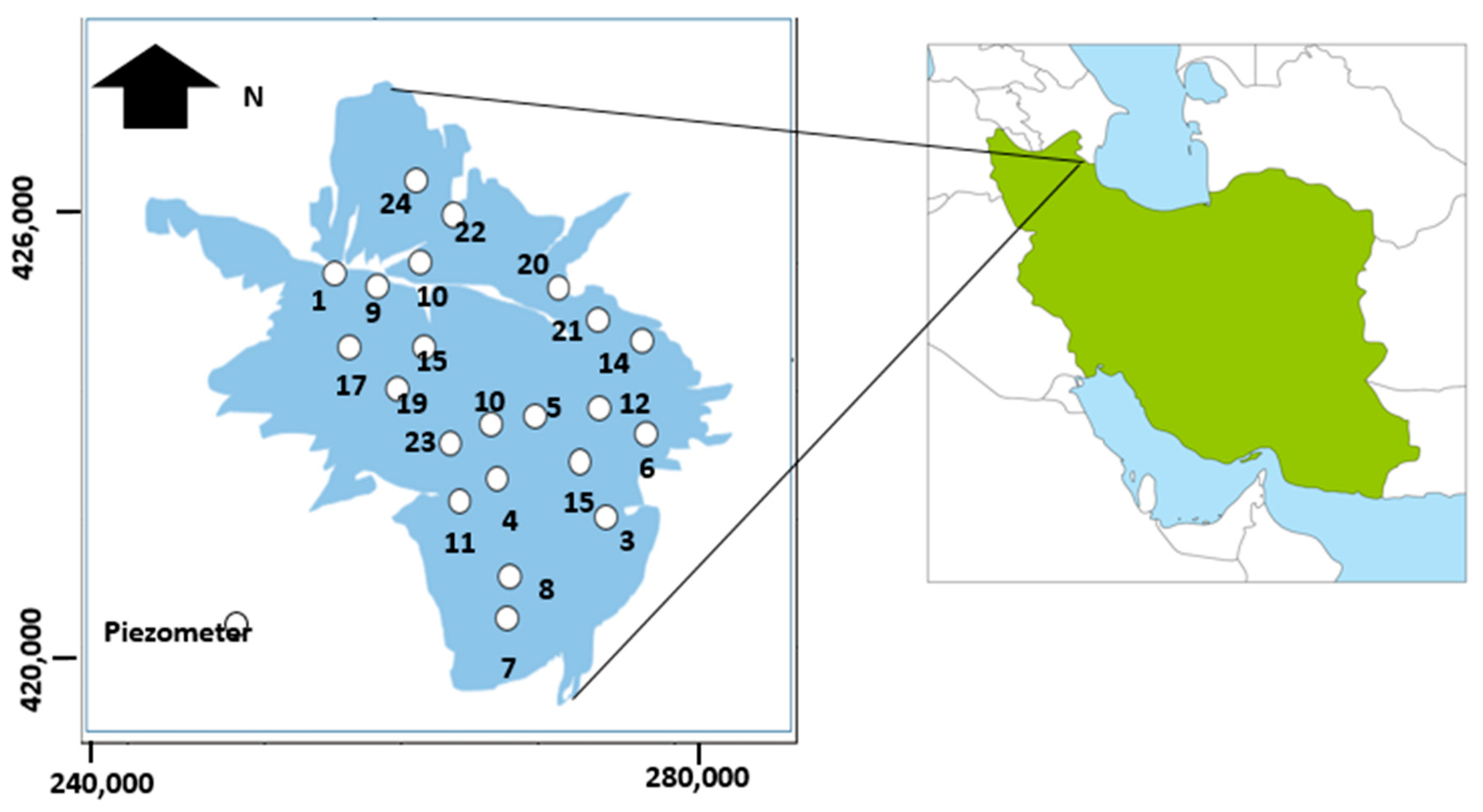
2.1. Case Study and Data
2.2. ANFIS Model
2.3. ANN Model
2.4. SVM Model
2.5. Optimization Algorithms
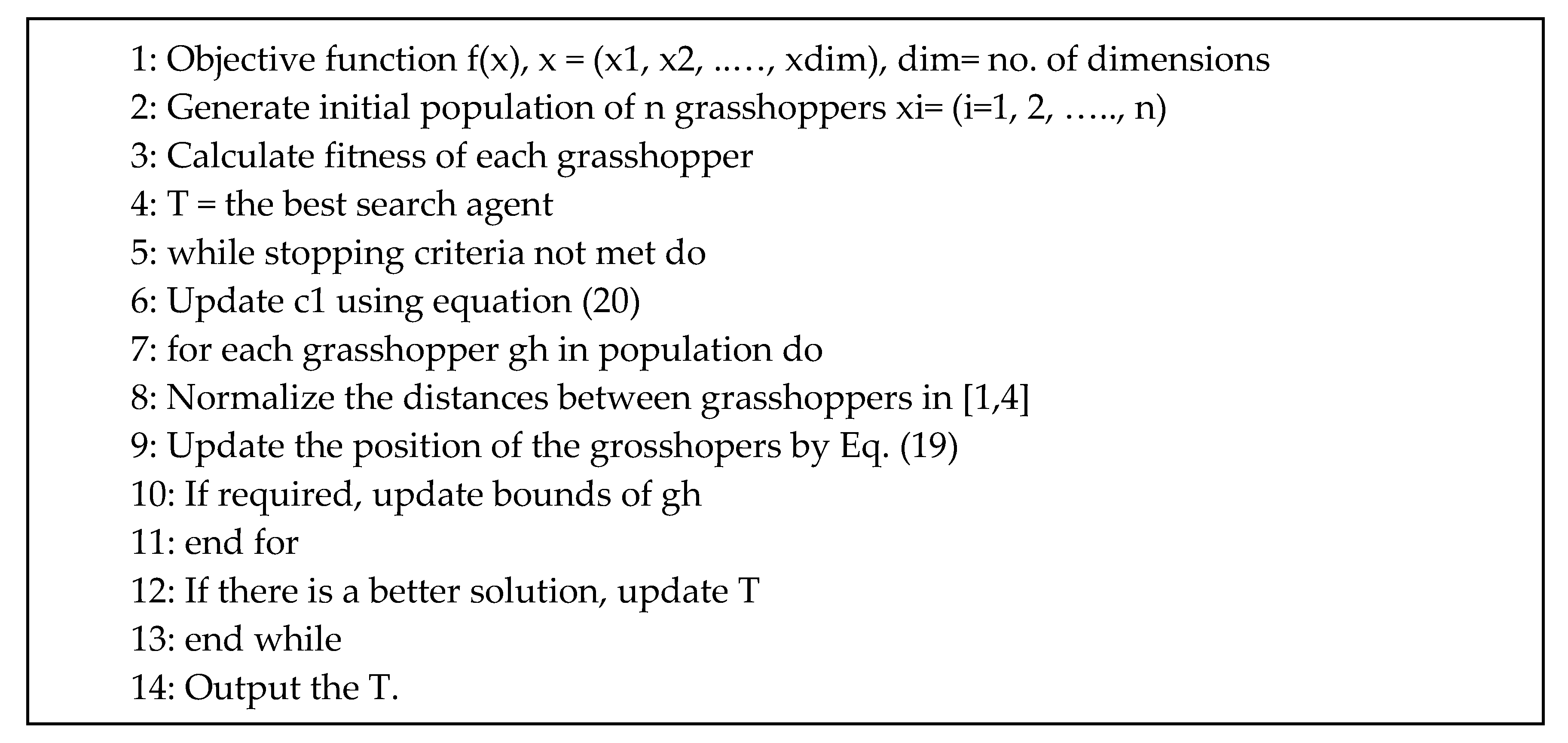
2.5.1. Grasshoppers Optimization Algorithm (GOA)
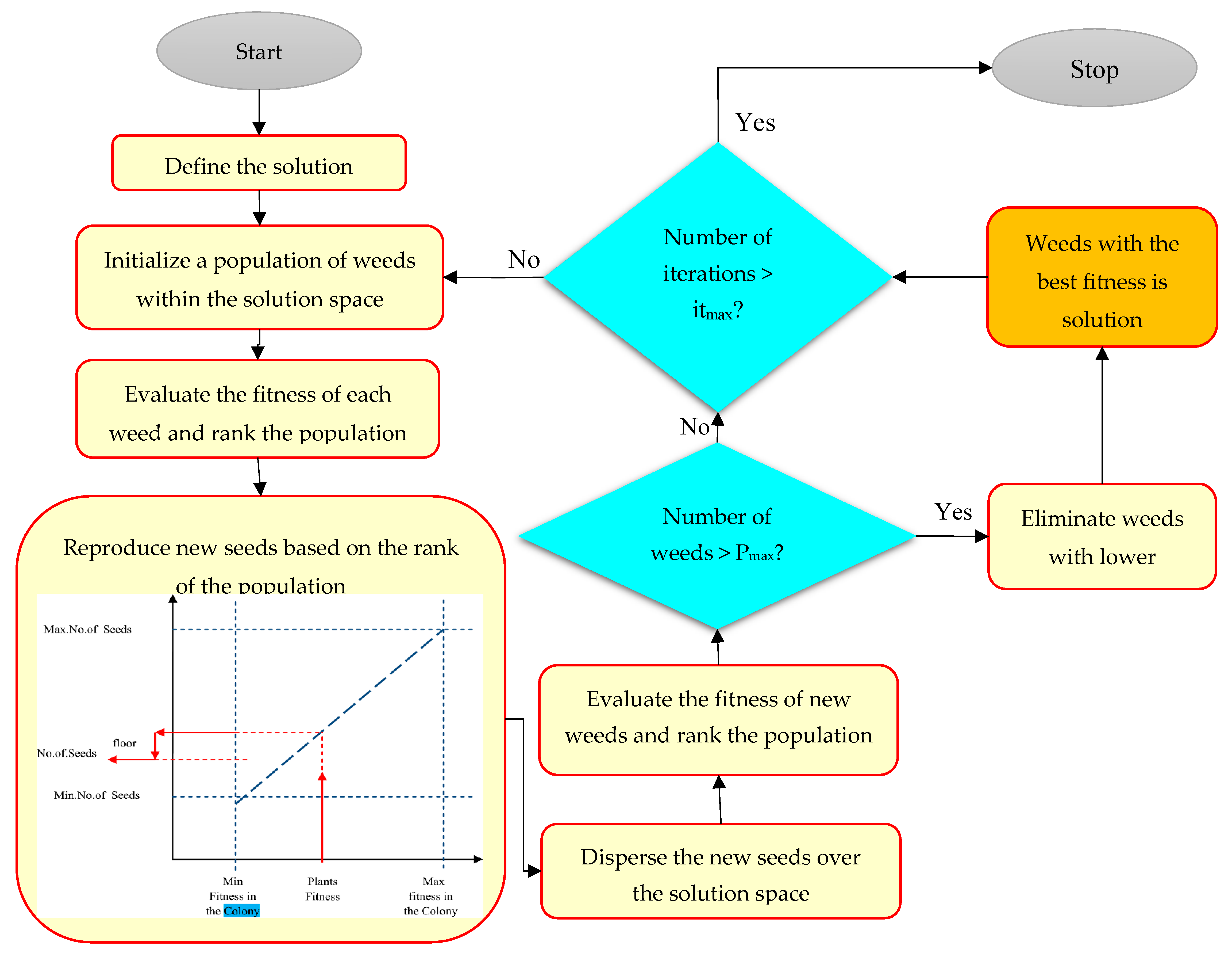
2.5.2. Weed Algorithm (WA)
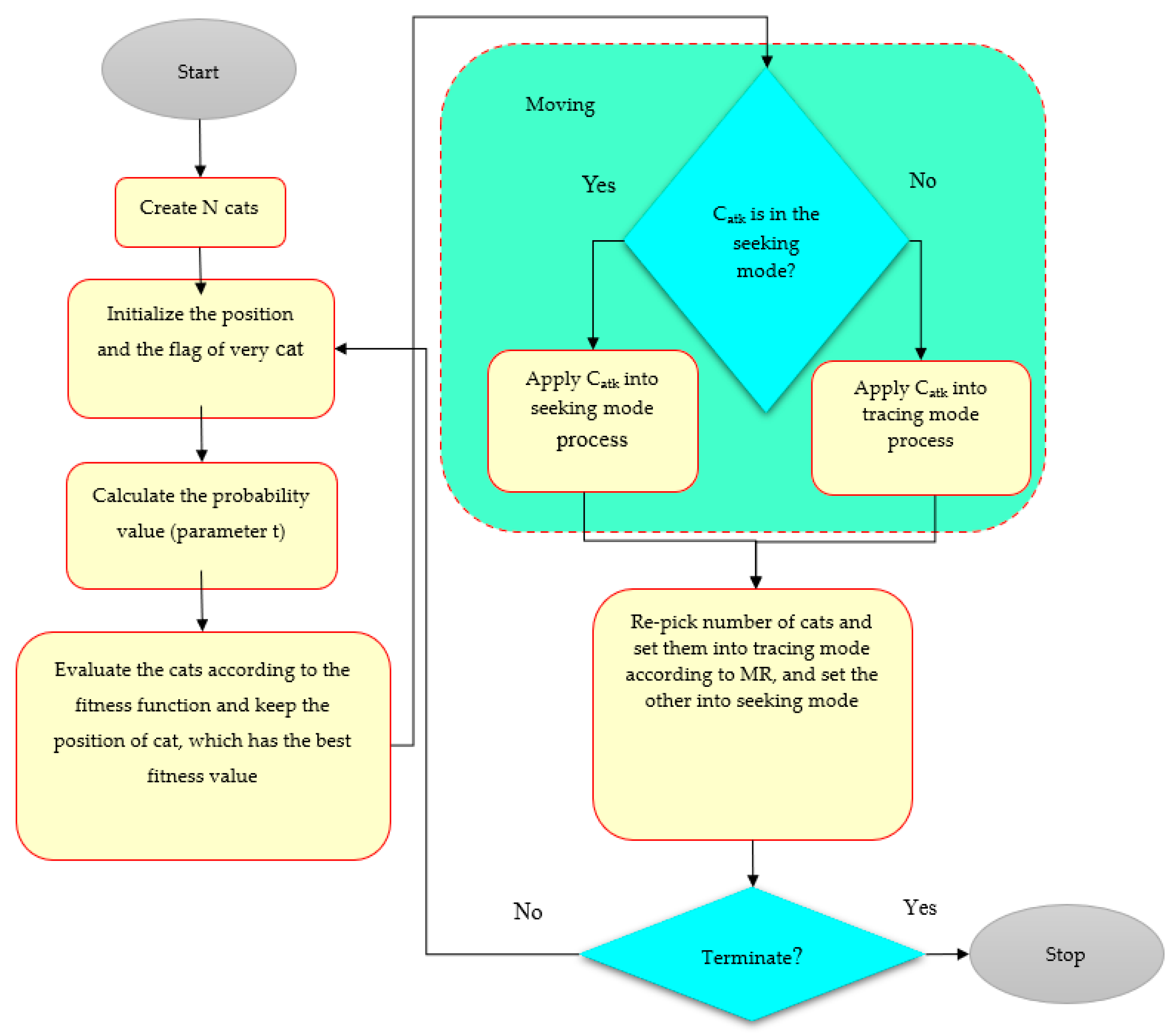
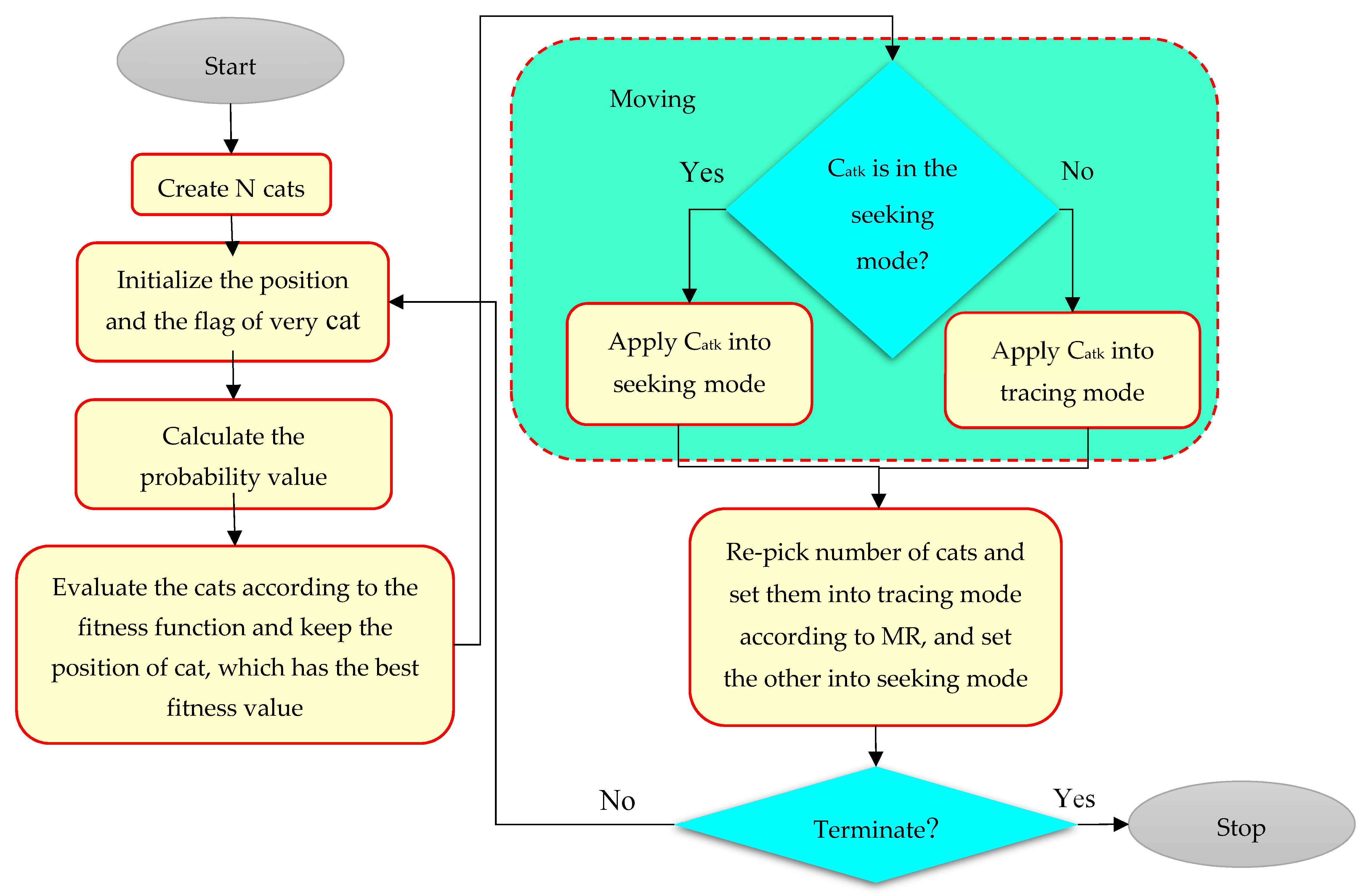
2.5.3. Cat Swarm Optimization (CSO)
- Generate replicas of the cats as per SMP.
- The position of each copy is updated as follows:where, is the position of the kth cat in the dth dimension (new position of the cat), is the random number, N is the number of cats, D is the number of dimensions, and is the position of jth cat in the d dimension (old position of the cat).
- Compute the objective function for all copies and choose the best objective function value (xbest) of the cat.
- Substitute xj,p with the best cat if the xbest is better than xj,p in terms of the objective function value.
2.5.4. Particle Swarm Optimization (PSO)
2.5.5. Genetic Algorithm (GA)
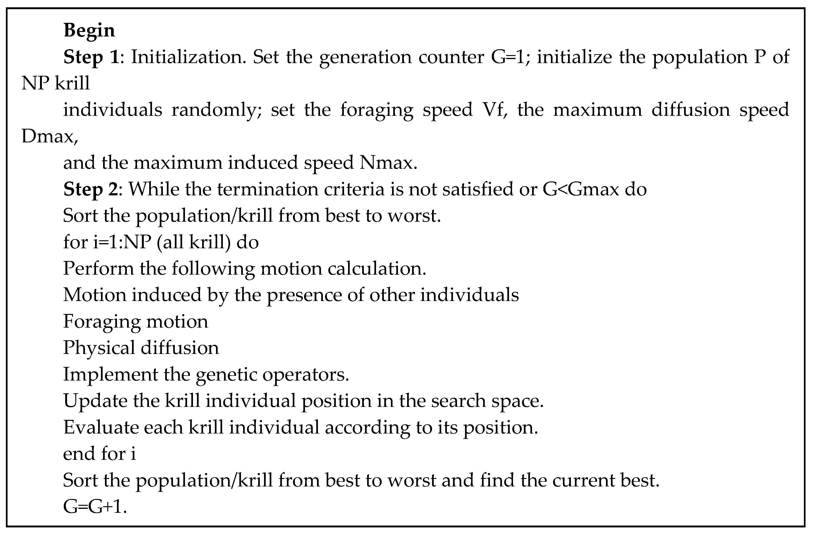
2.5.6. Krill Herd Algorithm (KHA)
2.6. Principal Component Analysis (PCA)
2.7. Taguchi Model
2.8. Hybrid ANN, ANFIS, and SVM Models with Optimization Algorithms
2.9. Uncertainty Analysis of Soft Computing Models
- A number of models are selected to simulate the GWL.
- The prior probability is assigned to each model.
- An error input model is defined.
- The posterior distribution of input error models and model parameters are obtained.
- A predetermined number of GWLs for each model is provided using probabilistic parameter estimations obtained from level 2 to level 4.
- The variance and weight of models are estimated.
- The weights for ensemble members of models are summed to compute the weight models.
- To the experimental soft computing models. The following indices were used to quantify the uncertainty of models:
2.10. Statistical Indices for Evaluation of Different Models
3. Results and Discussion
3.1. Inputs Selection by PCA
3.2. Selection of Random Parameters by the Taguchi Model
3.3. Results of Hybrid ANN, ANFIS, and SVM Models
- piezometer 6
- piezometer 9
- piezometer 10
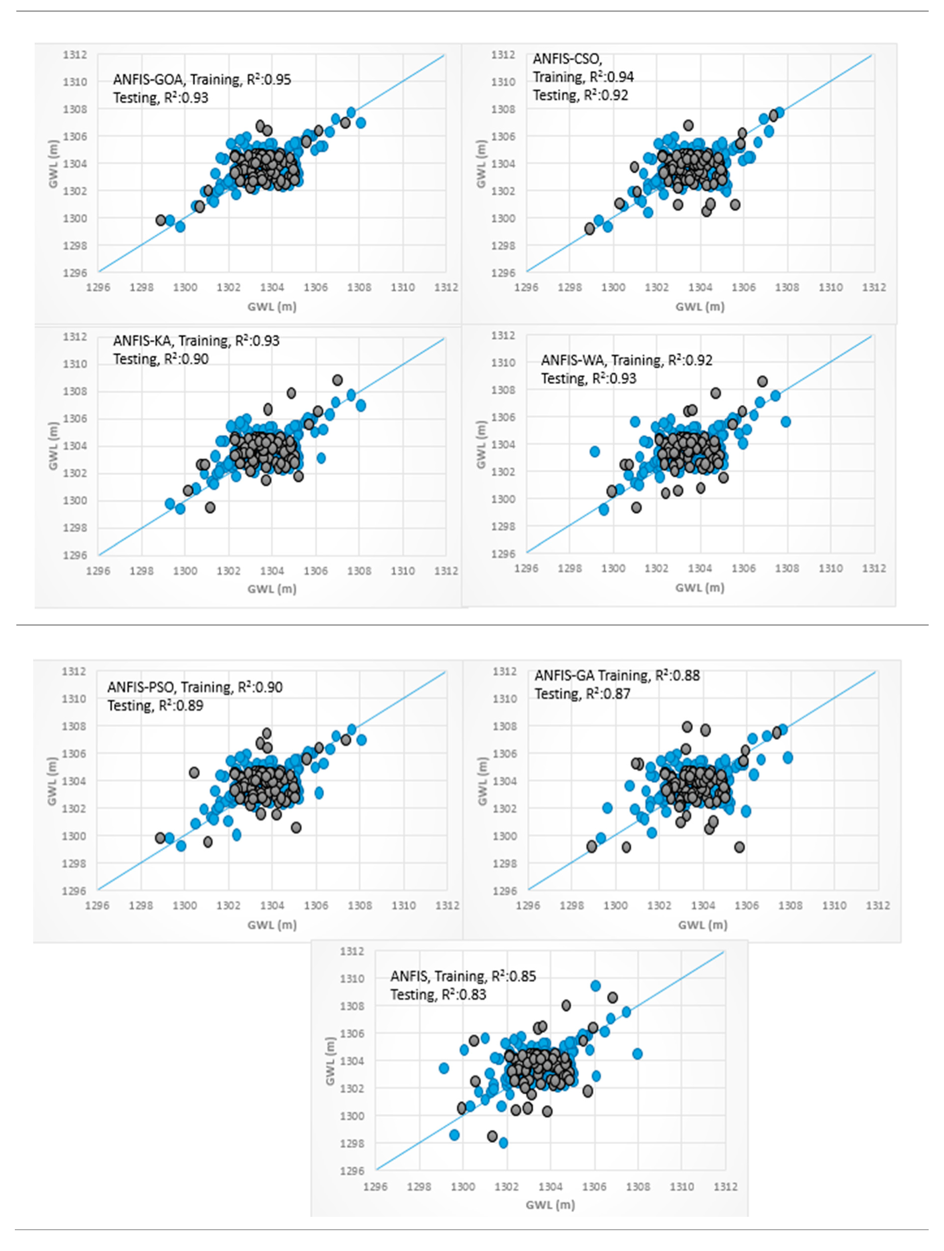
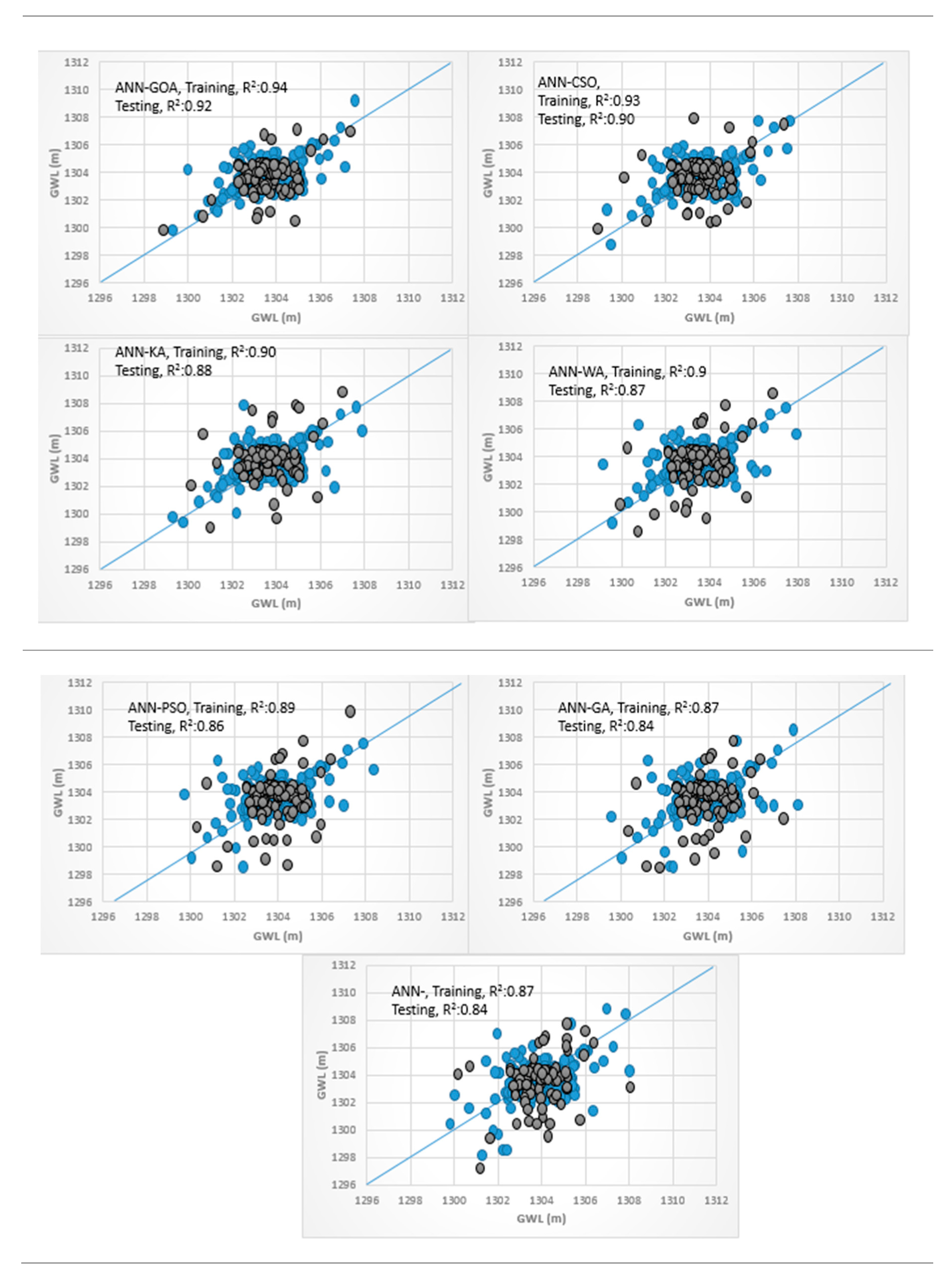
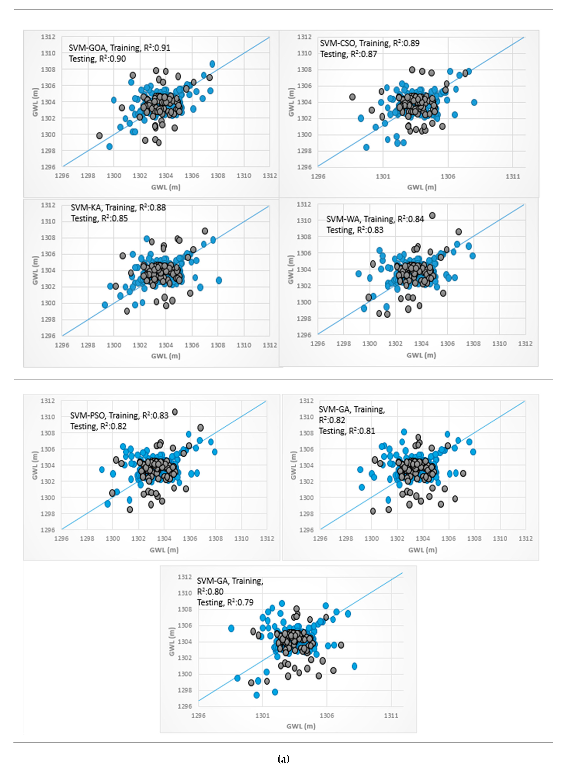
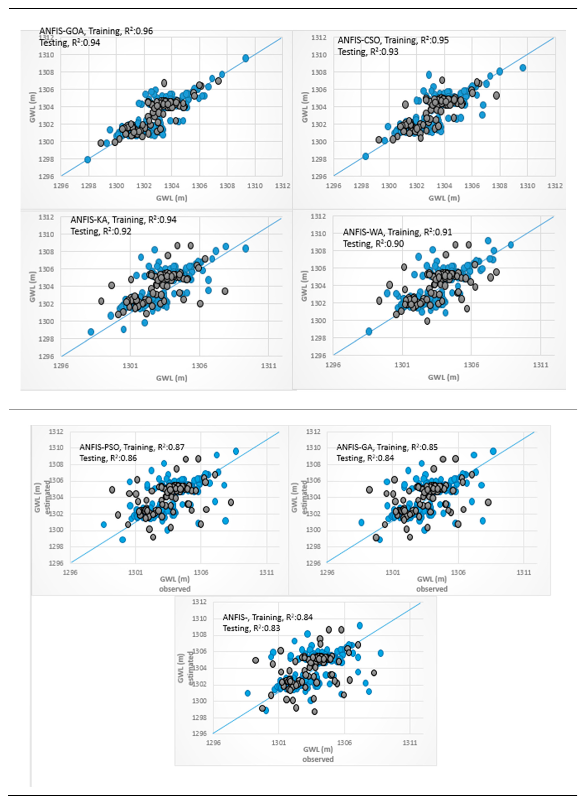
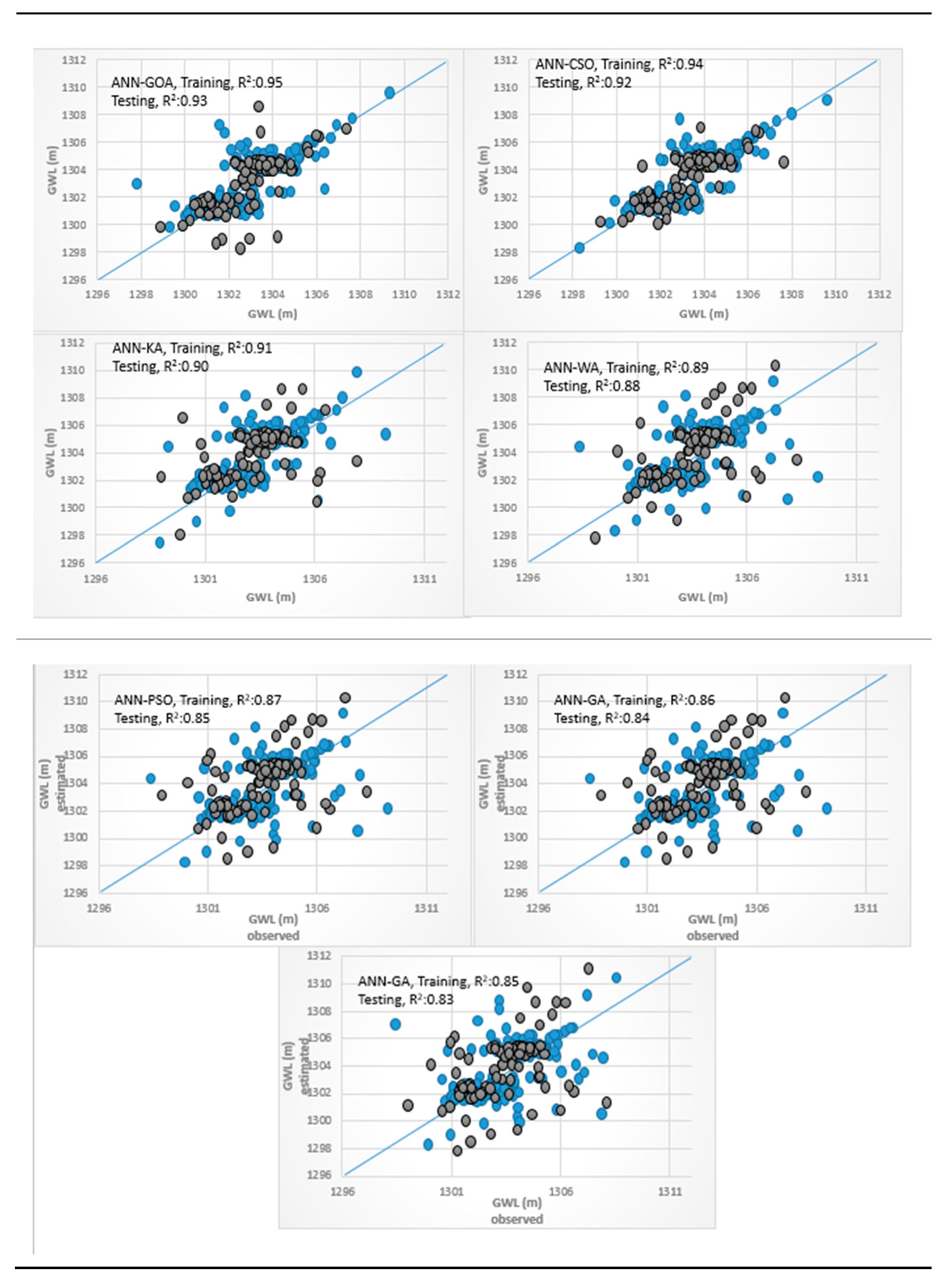
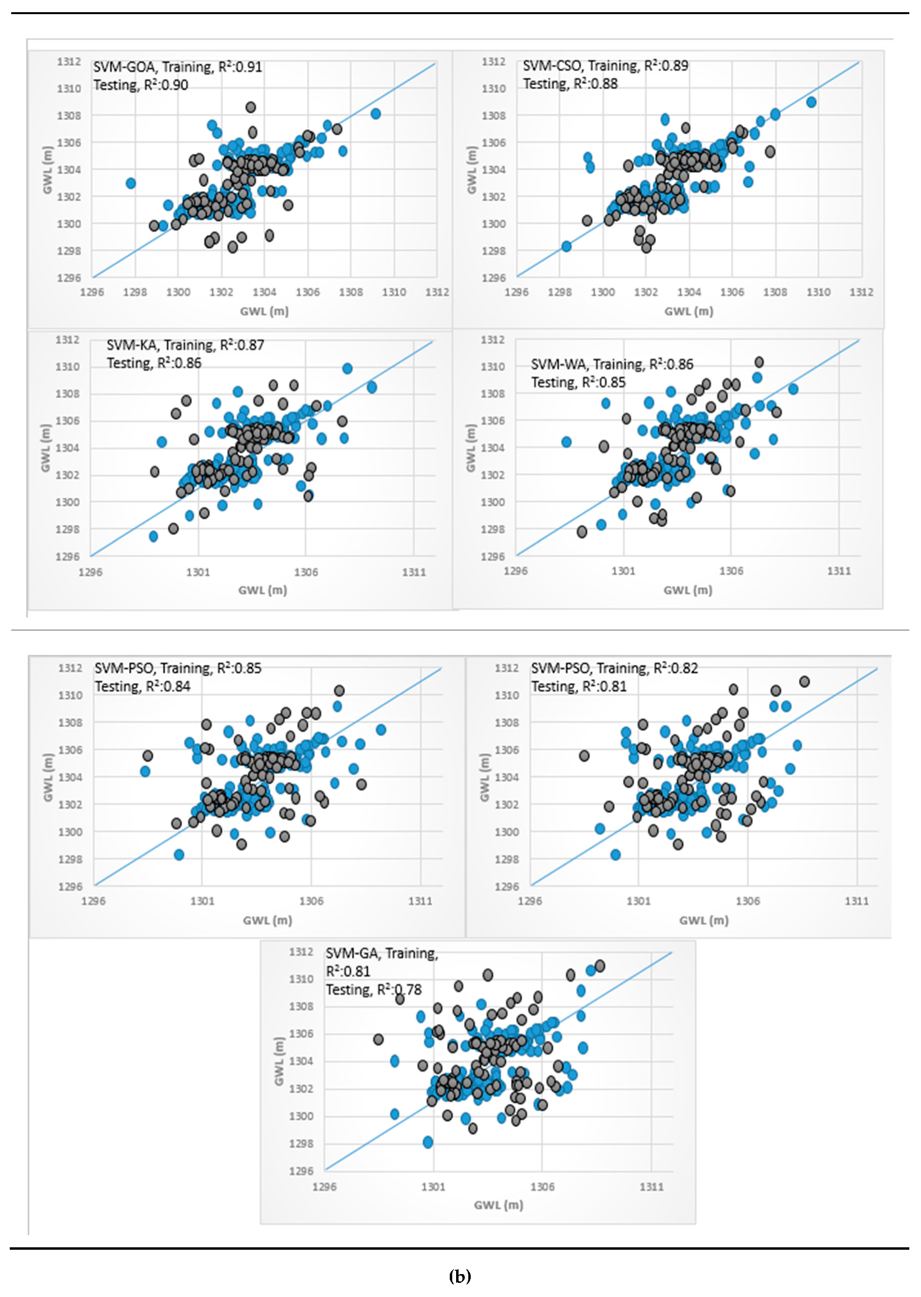
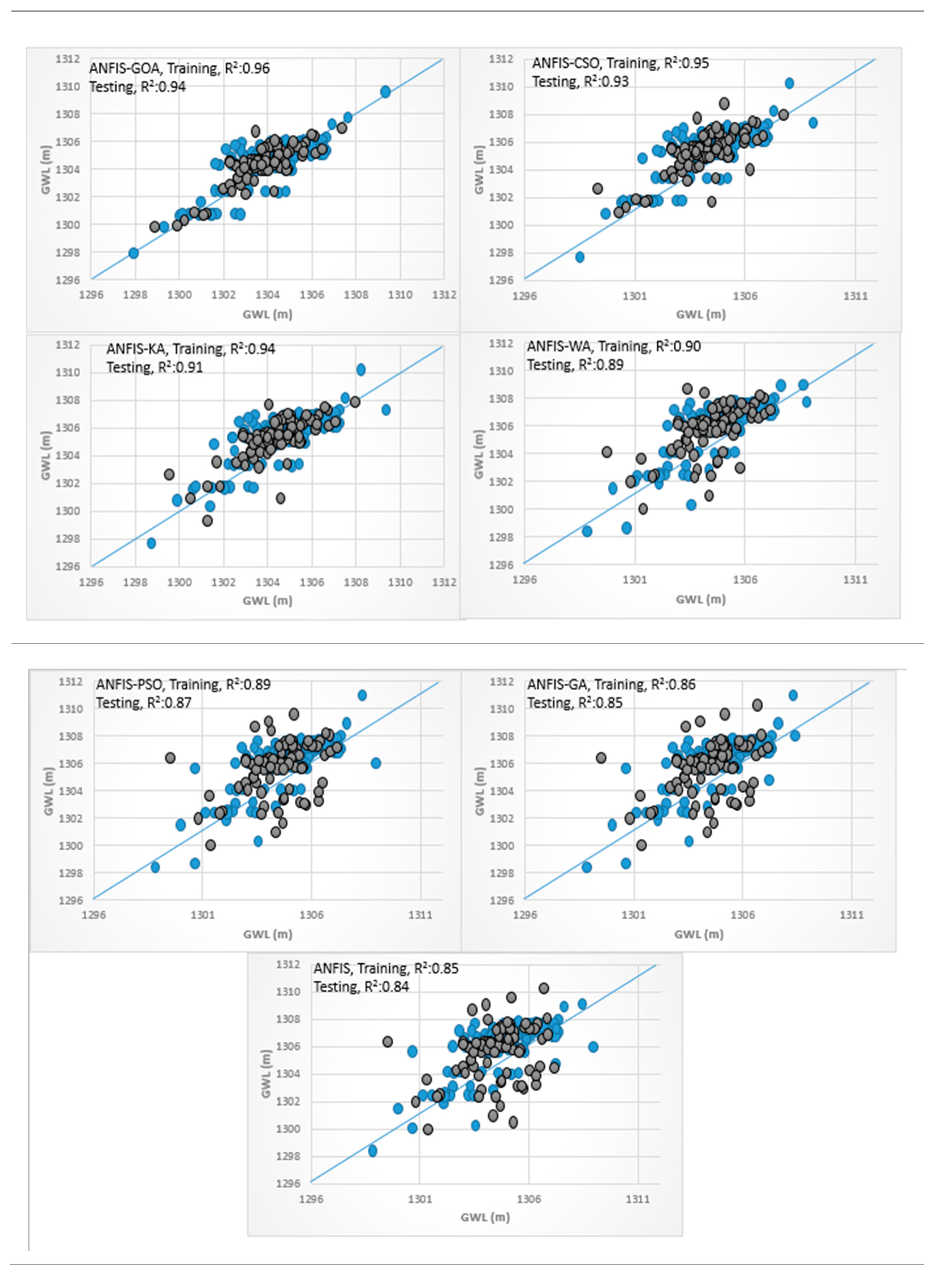
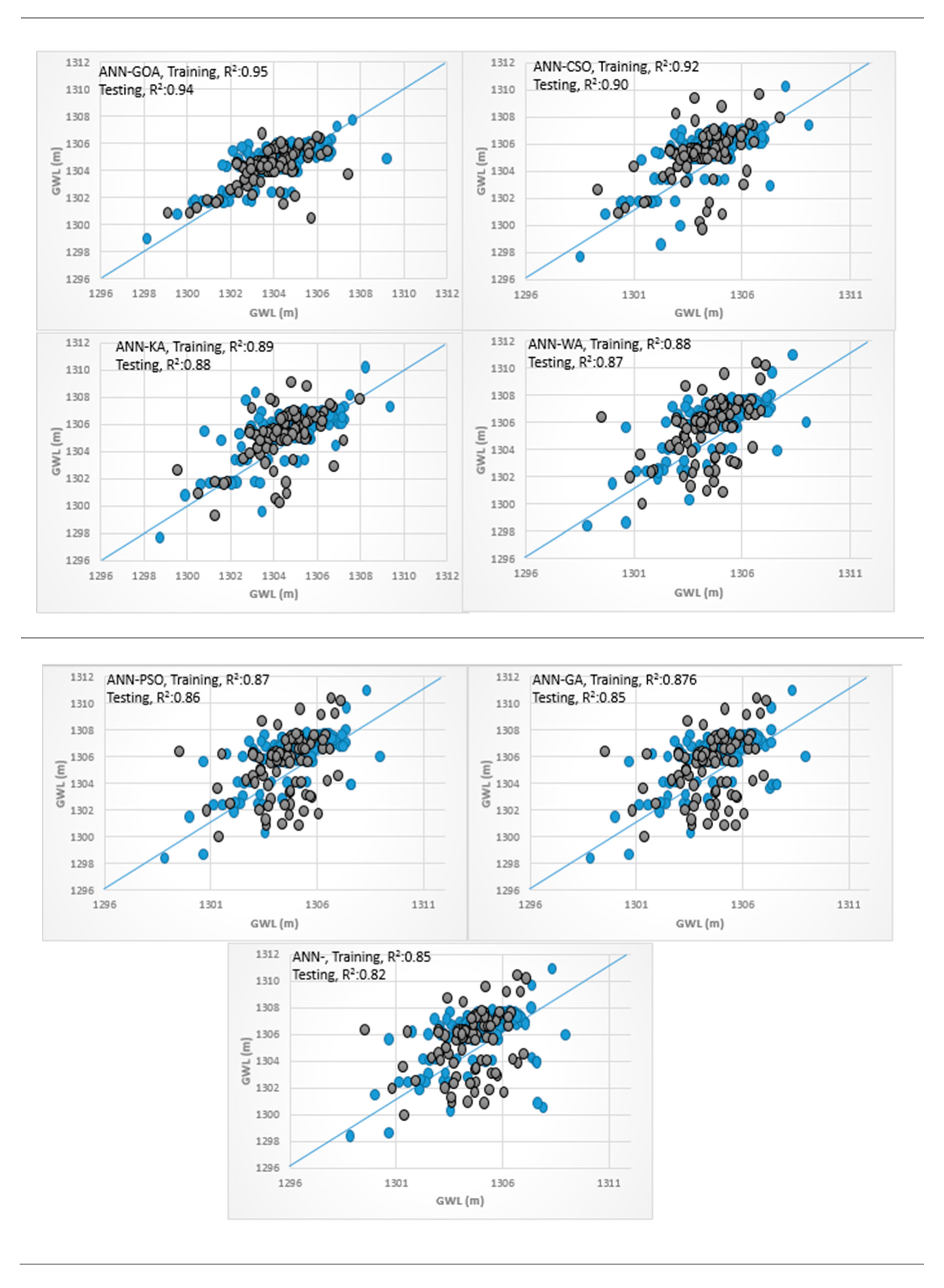
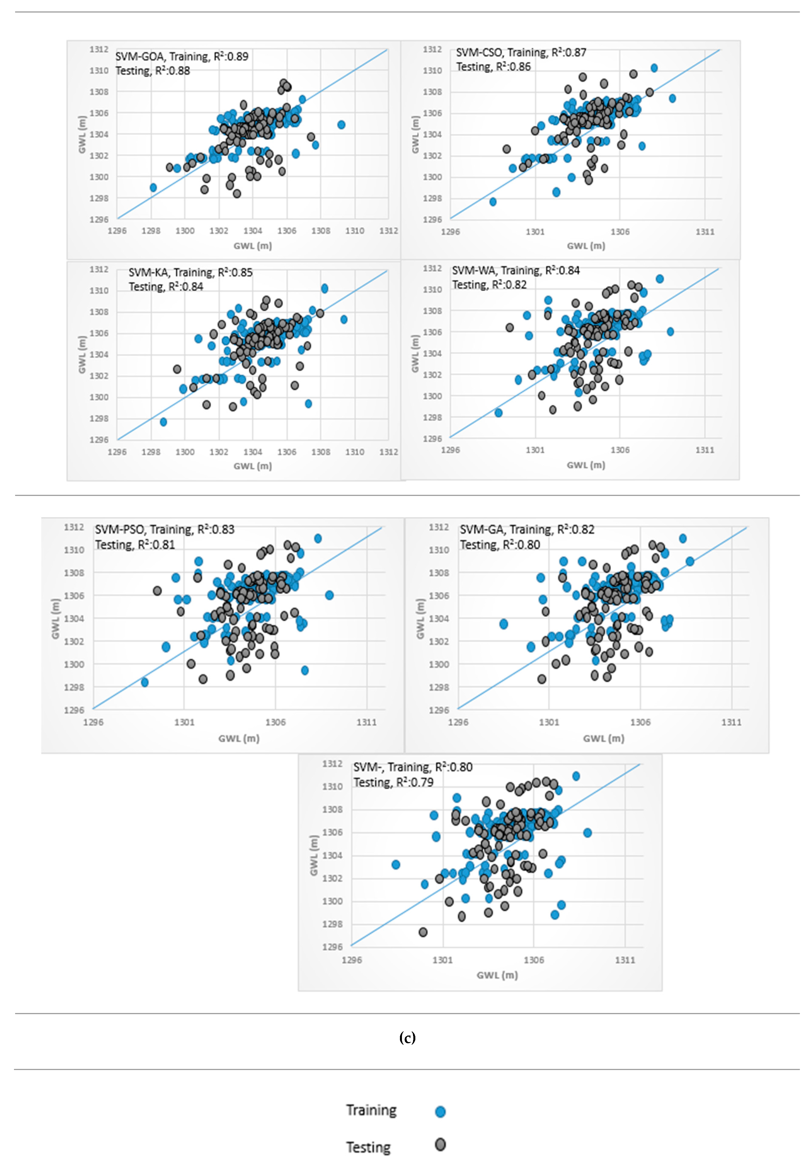
3.4. Analysis of Scatterplots of Soft Computing Models
- piezometer 6
- piezometer 9
- Piezometer 10
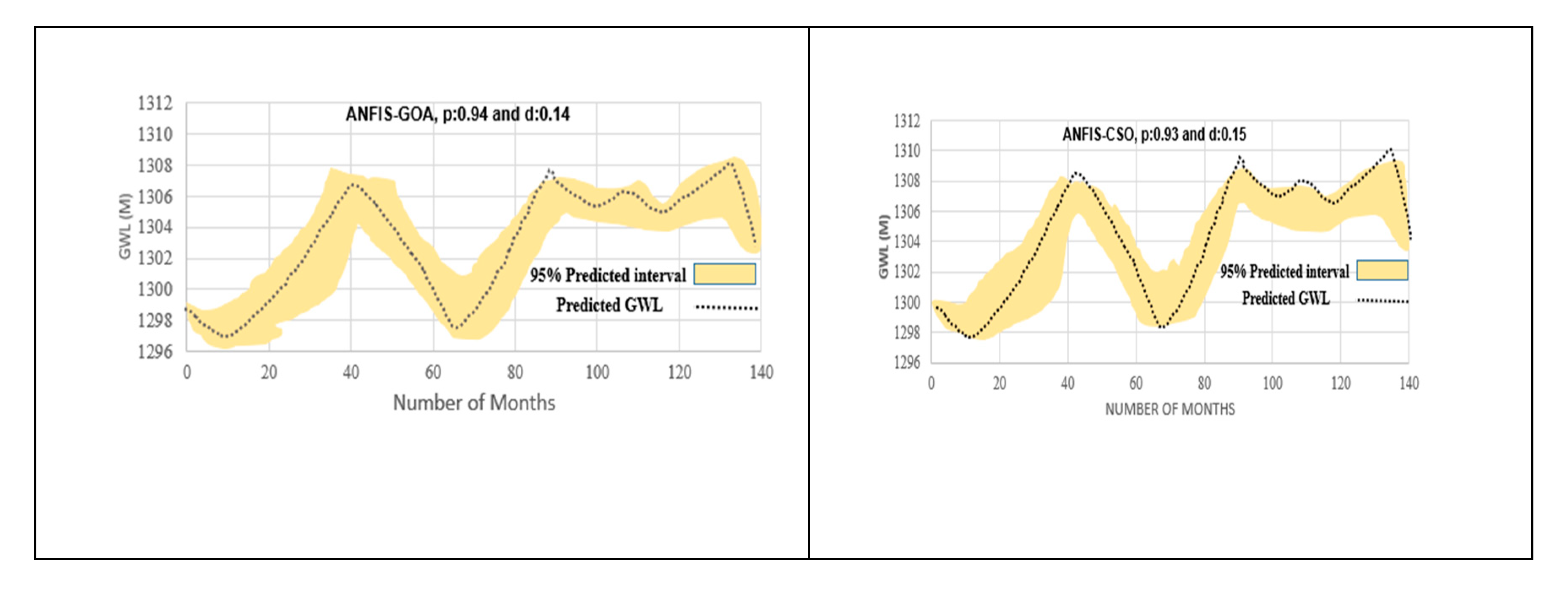
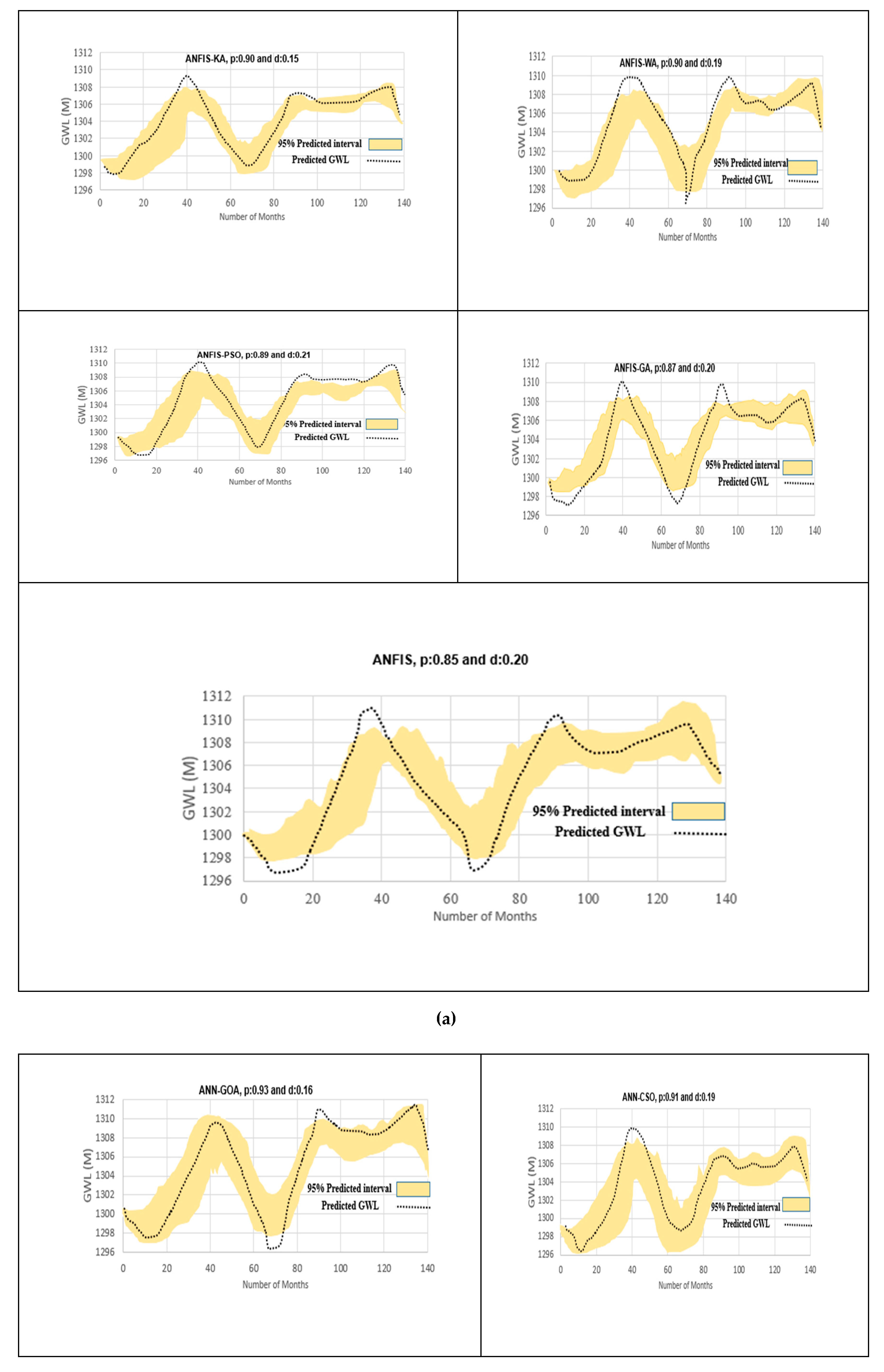
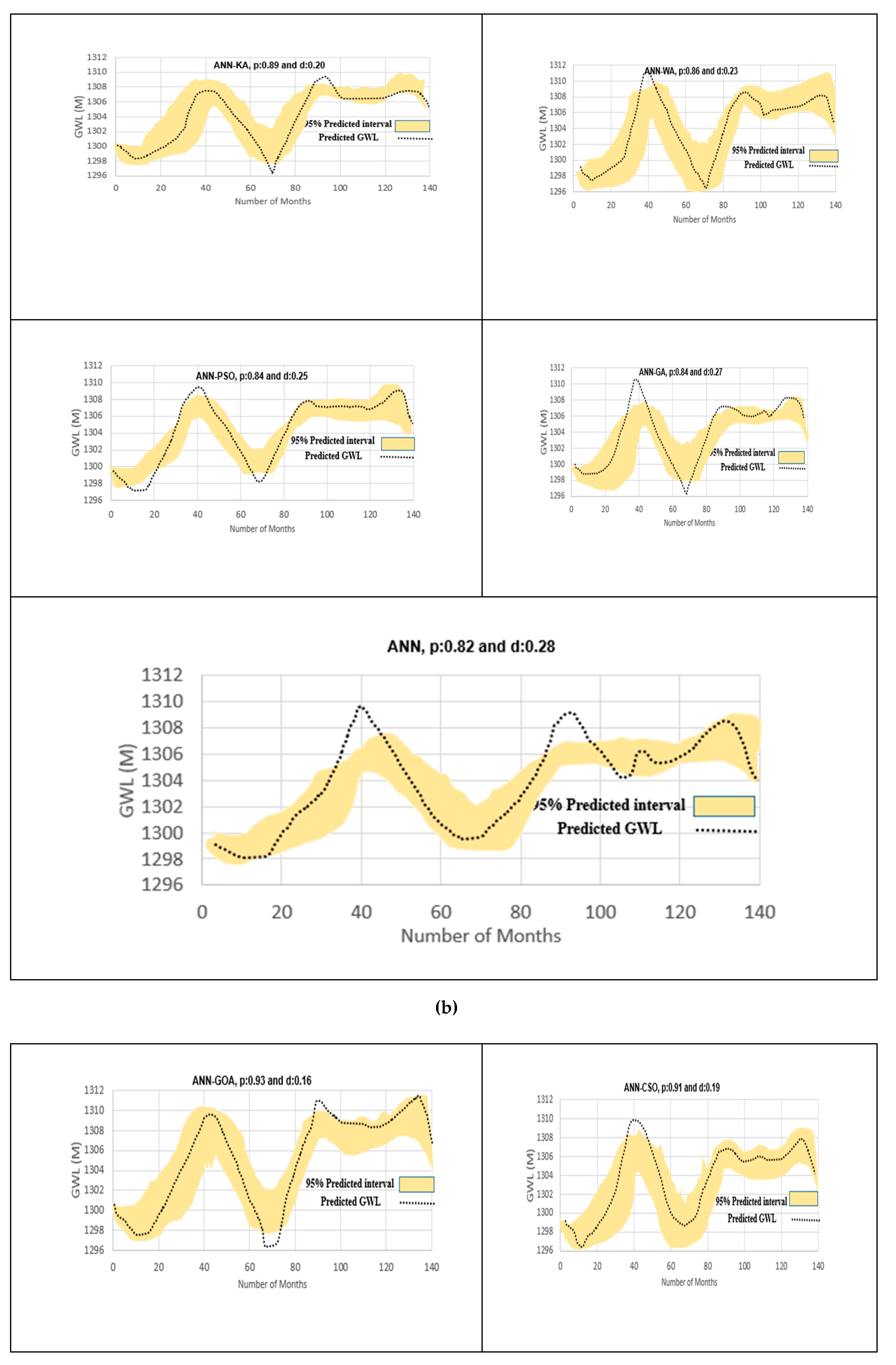
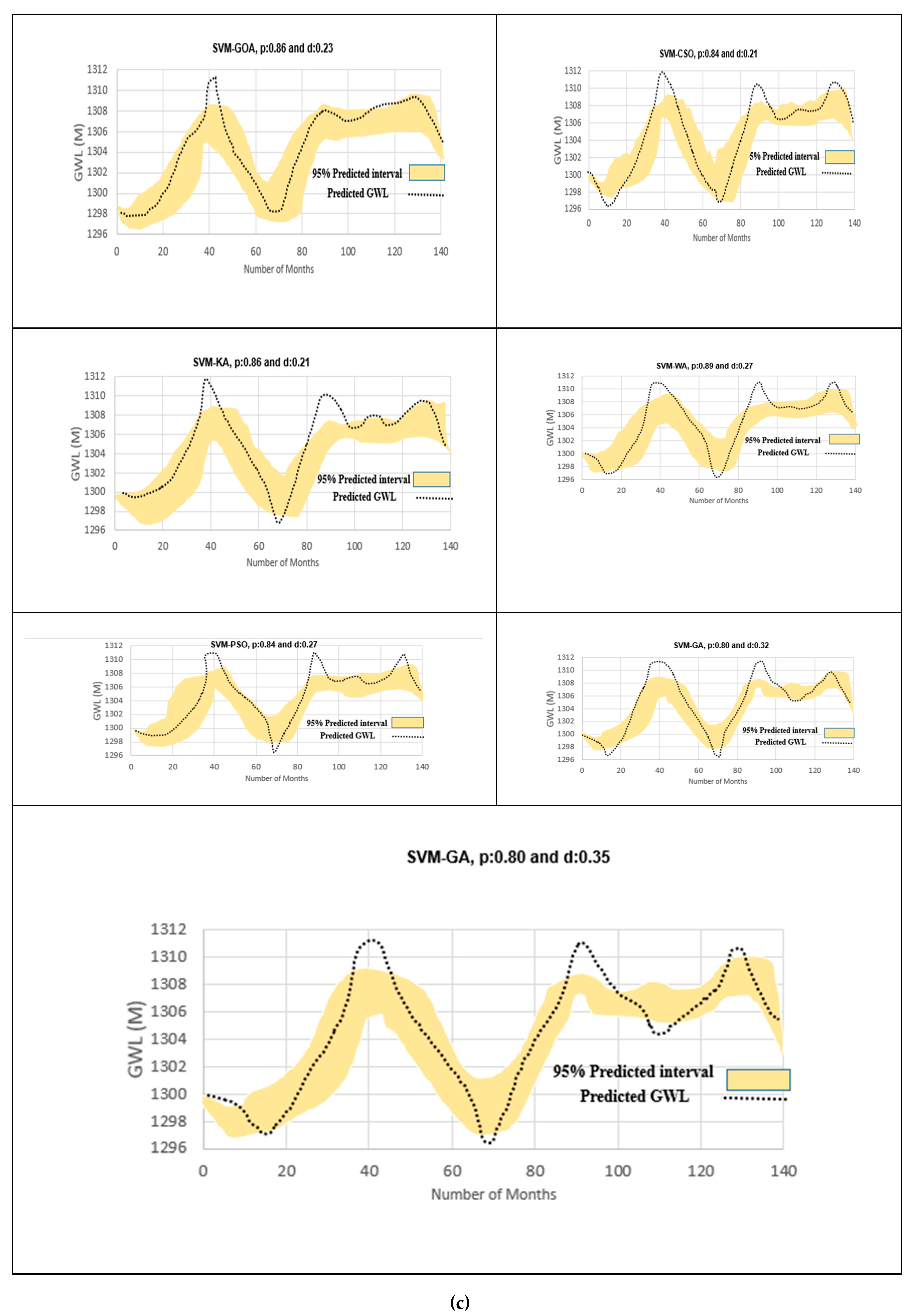
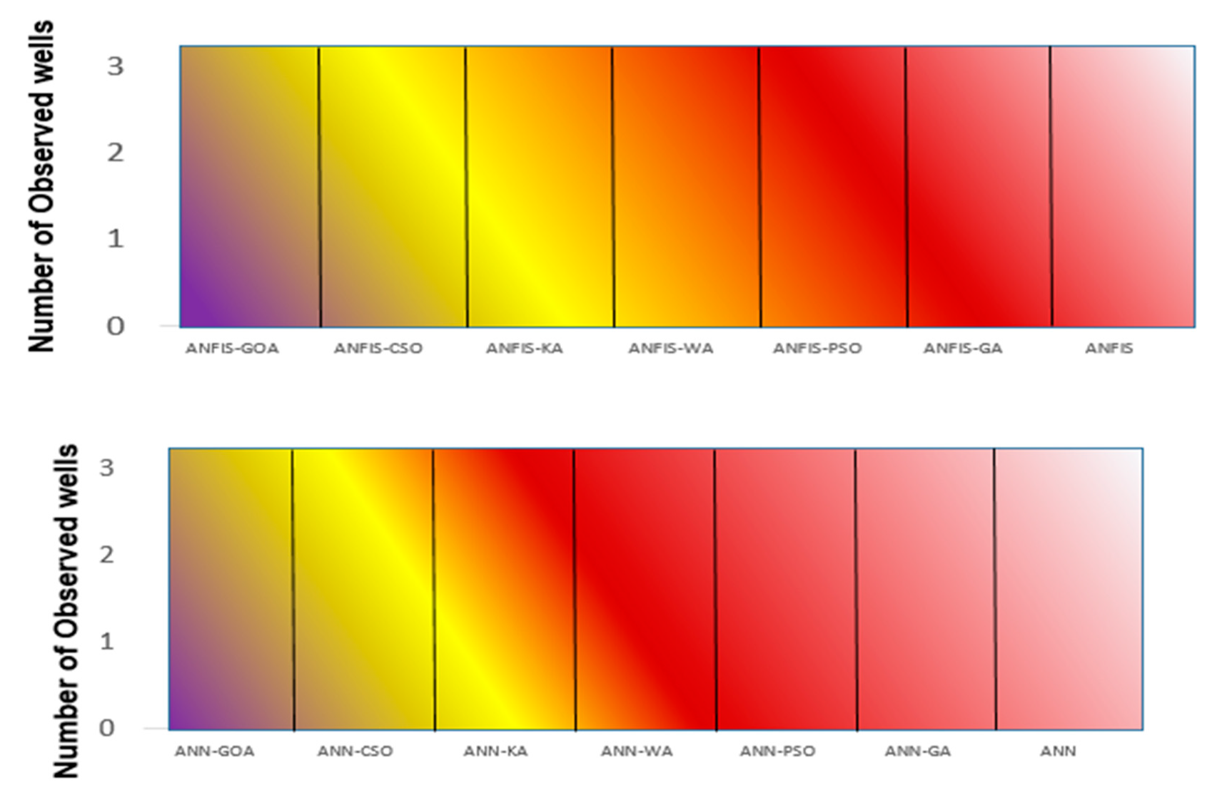
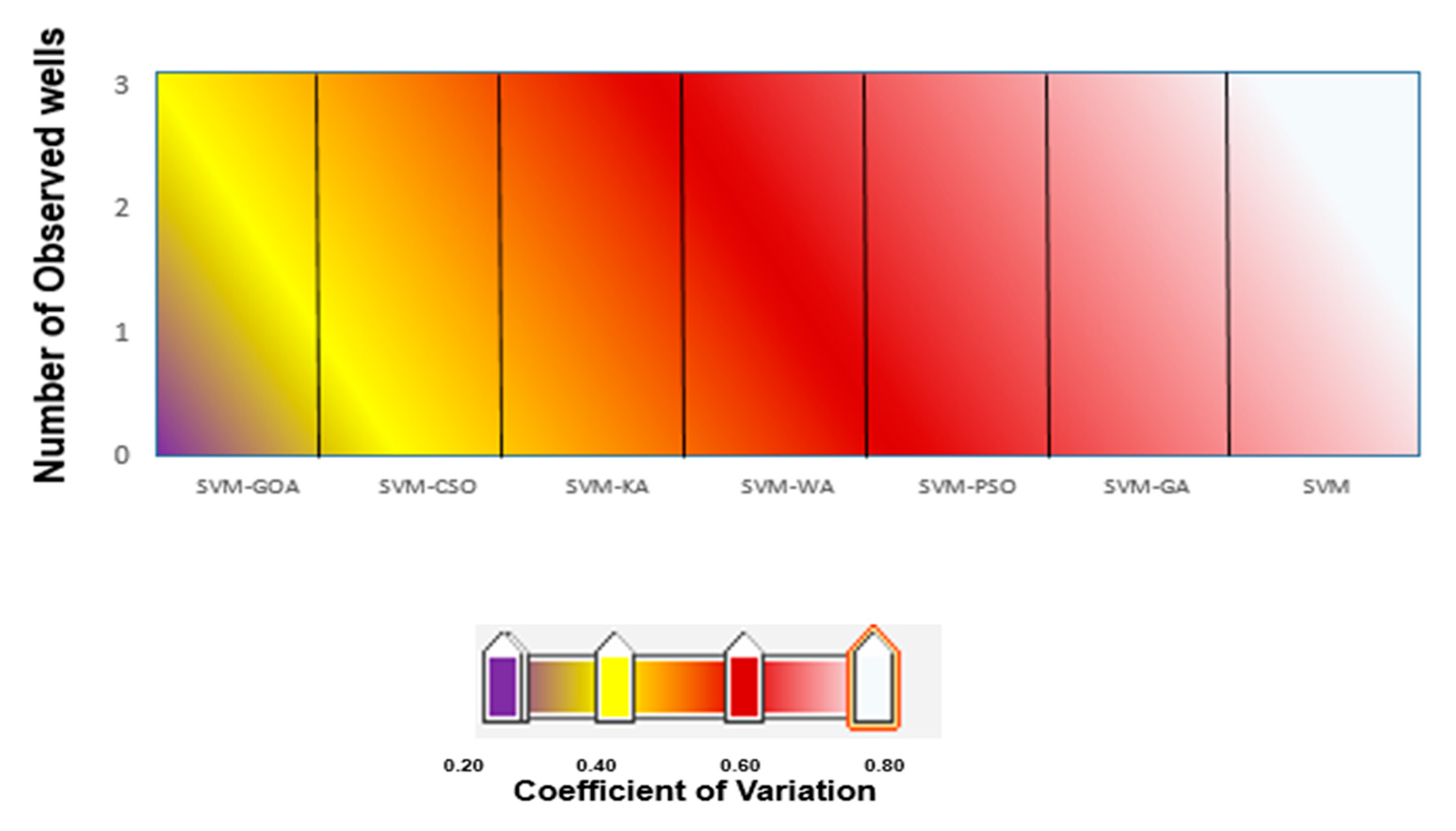
3.5. Uncertainty Analysis of Soft Computing Models
- Piezometer 6
- Piezometer 9
- Piezometer 10
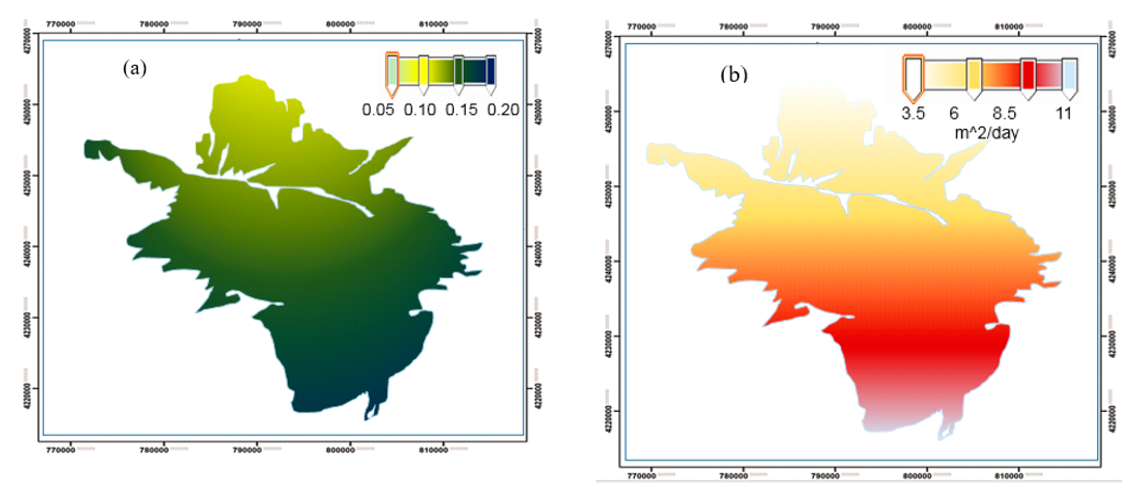
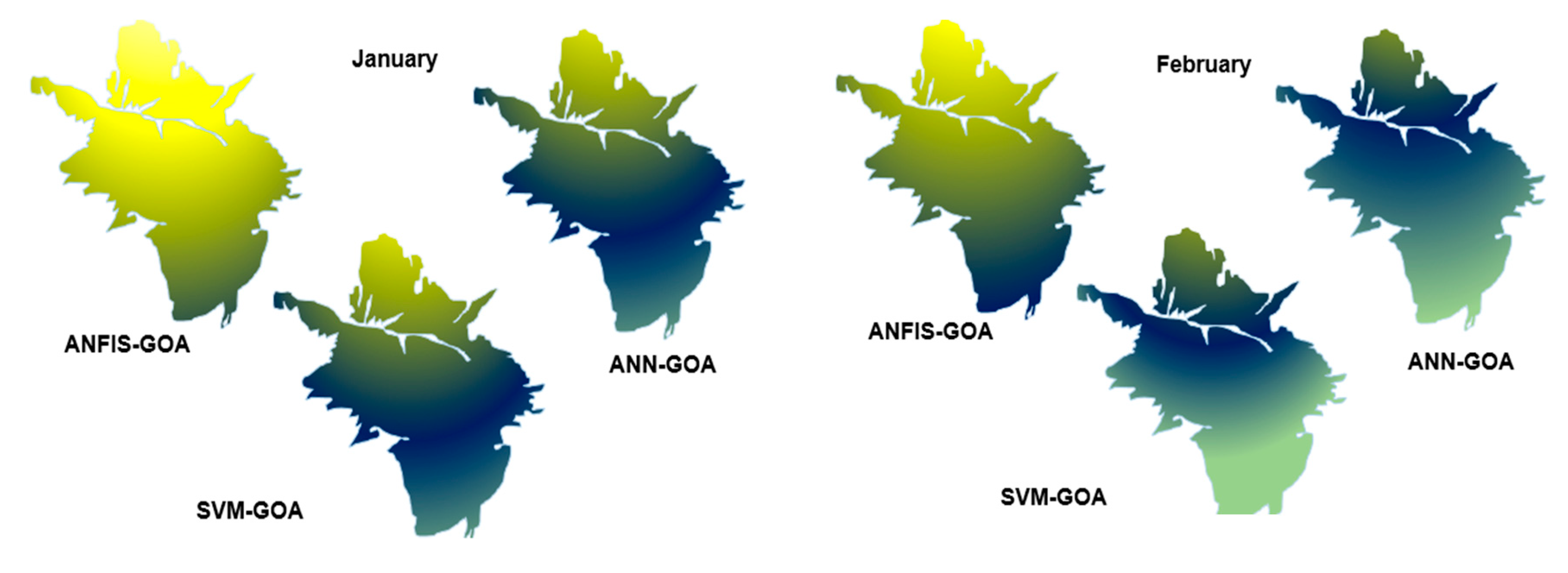
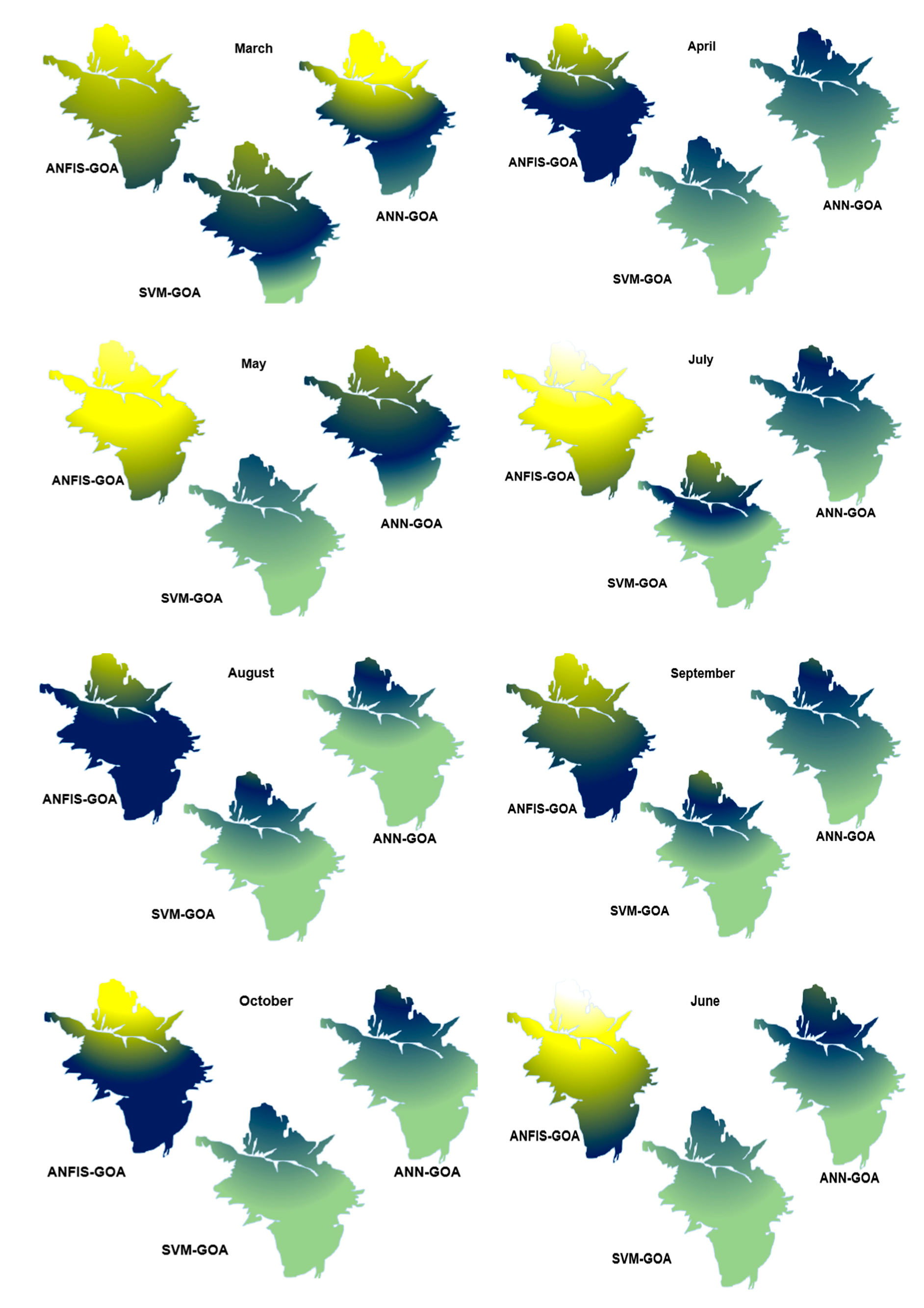
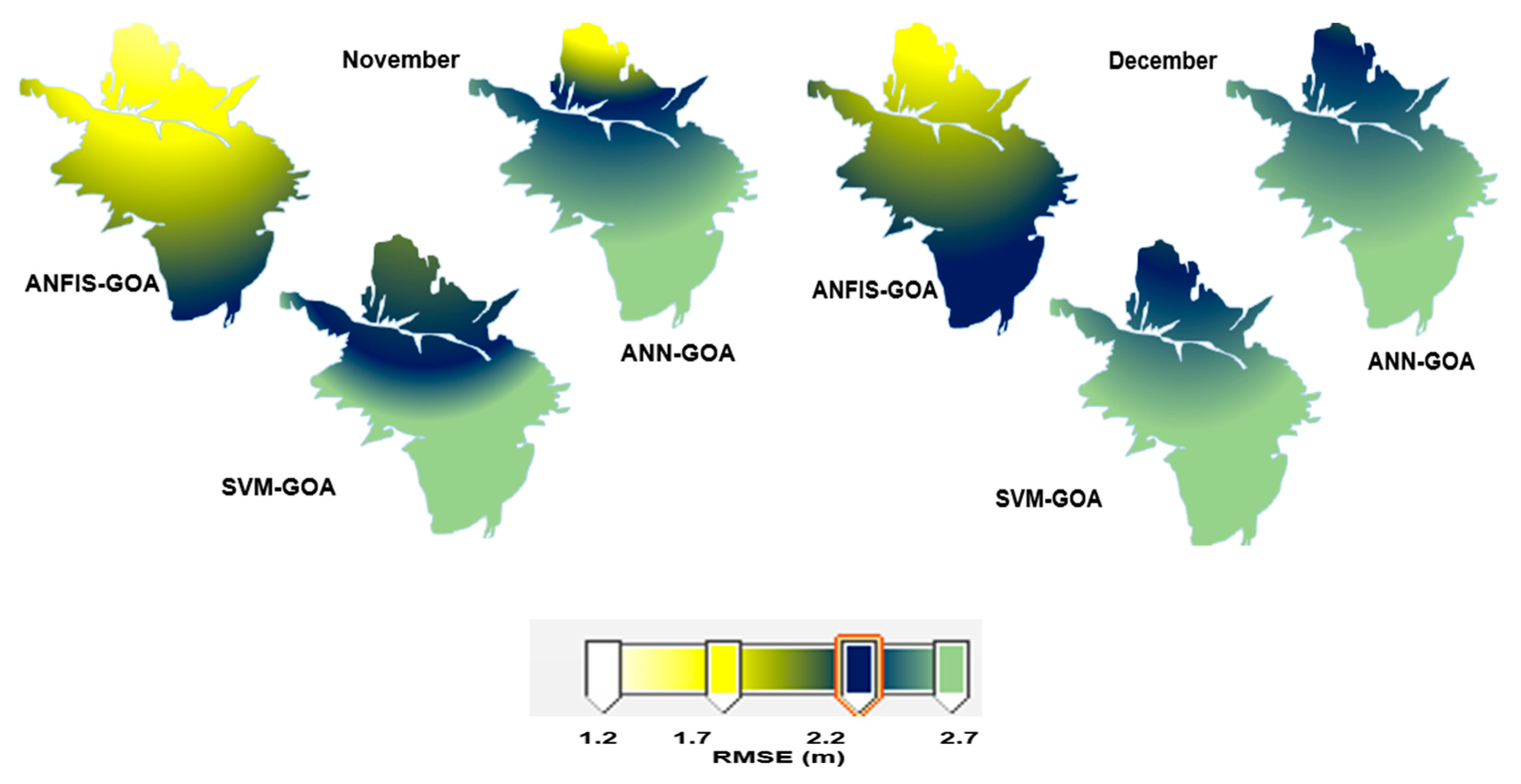
3.6. Spatiotemporal Variation of GWL
4. Conclusions
Author Contributions
Funding
Acknowledgments
Conflicts of Interest
References
- Sattari, M.T.; Mirabbasi, R.; Sushab, R.S.; Abraham, J. Prediction of Groundwater Level in Ardebil Plain Using Support Vector Regression and M5 Tree Model. Groundwater 2018. [Google Scholar] [CrossRef] [PubMed]
- Jeong, J.; Park, E. Comparative applications of data-driven models representing water table fluctuations. J. Hydrol. 2019, 572, 261–273. [Google Scholar] [CrossRef]
- Alizamir, M.; Kisi, O.; Zounemat-Kermani, M. Modelling long-term groundwater fluctuations by extreme learning machine using hydro-climatic data. Hydrol. Sci. J. 2018, 63, 63–73. [Google Scholar] [CrossRef]
- Yoon, H.; Kim, Y.; Lee, S.H.; Ha, K. Influence of the range of data on the performance of ANN-and SVM-based time series models for reproducing groundwater level observations. Acque Sotter. Ital. J. Groundwater. 2019. [Google Scholar] [CrossRef]
- Mohanty, S.; Jha, M.K.; Kumar, A.; Sudheer, K.P. Artificial neural network modeling for groundwater level forecasting in a river island of eastern India. Water Resour. Manag. 2010, 24, 1845–1865. [Google Scholar] [CrossRef]
- Natarajan, N.; Sudheer, C. Groundwater level forecasting using soft computing techniques. Neural Comput. Appl. 2019, 1–18. [Google Scholar] [CrossRef]
- Lee, S.; Lee, K.K.; Yoon, H. Using artificial neural network models for groundwater level forecasting and assessment of the relative impacts of influencing factors. Hydrogeol. J. 2019, 27, 567–579. [Google Scholar] [CrossRef]
- Khan, U.T.; Valeo, C. Dissolved oxygen prediction using a possibility theory based fuzzy neural network. Hydrol. Earth Syst. Sci. 2016, 20, 2267–2293. [Google Scholar] [CrossRef]
- Jeihouni, E.; Eslamian, S.; Mohammadi, M.; Zareian, M.J. Simulation of groundwater level fluctuations in response to main climate parameters using a wavelet–ANN hybrid technique for the Shabestar Plain, Iran. Environ. Earth Sci. 2019, 78, 293. [Google Scholar] [CrossRef]
- Alian, S.; Mayer, A.; Maclean, A.; Watkins, D.; Mirchi, A. Spatiotemporal Dimensions of Water Stress Accounting: Incorporating Groundwater–Surface Water Interactions and Ecological Thresholds. Environ. Sci. Technol. 2019, 53, 2316–2323. [Google Scholar] [CrossRef]
- Jalalkamali, A.; Sedghi, H.; Manshouri, M. Monthly groundwater level prediction using ANN and neuro-fuzzy models: A case study on Kerman plain, Iran. J. Hydroinformatics. 2010, 13, 867–876. [Google Scholar] [CrossRef]
- Trichakis, I.C.; Nikolos, I.K.; Karatzas, G.P. Artificial neural network (ANN) based modeling for karstic groundwater level simulation. Water Resour. Manag. 2011, 25, 1143–1152. [Google Scholar] [CrossRef]
- Fallah-Mehdipour, E.; Haddad, O.B.; Mariño, M.A. Prediction and simulation of monthly groundwater levels by genetic programming. J Hydro-Environment. Res. 2013, 7, 253–260. [Google Scholar] [CrossRef]
- Moosavi, V.; Vafakhah, M.; Shirmohammadi, B.; Behnia, N. A wavelet-ANFIS hybrid model for groundwater level forecasting for different prediction periods. Water Resour. Manag. 2013, 27, 1301–1321. [Google Scholar] [CrossRef]
- Emamgholizadeh, S.; Moslemi, K.; Karami, G. Prediction the Groundwater Level of Bastam Plain (Iran) by Artificial Neural Network (ANN) and Adaptive Neuro-Fuzzy Inference System (ANFIS). Water Resour. Manag. 2014, 28, 5433–5446. [Google Scholar] [CrossRef]
- Suryanarayana, C.; Sudheer, C.; Mahammood, V.; Panigrahi, B.K. An integrated wavelet-support vector machine for groundwater level prediction in Visakhapatnam, India. Neurocomputing 2014, 145, 324–335. [Google Scholar] [CrossRef]
- Mohanty, S.; Jha, M.K.; Raul, S.K.; Panda, R.K.; Sudheer, K.P. Using artificial neural network approach for simultaneous forecasting of weekly groundwater levels at multiple sites. Water Resour. Manag. 2015, 29, 5521–5532. [Google Scholar] [CrossRef]
- Yoon, H.; Hyun, Y.; Ha, K.; Lee, K.K.; Kim, G.B. A method to improve the stability and accuracy of ANN-and SVM-based time series models for long-term groundwater level predictions. Comput. Geosci. 2016, 90, 144–155. [Google Scholar] [CrossRef]
- Zhou, T.; Wang, F.; Yang, Z. Comparative analysis of ANN and SVM models combined with wavelet preprocess for groundwater depth prediction. Water 2017, 9, 781. [Google Scholar] [CrossRef]
- Choubin, B.; Malekian, A. Combined gamma and M-test-based ANN and ARIMA models for groundwater fluctuation forecasting in semiarid regions. Environ. Earth Sci. 2017, 76, 538. [Google Scholar] [CrossRef]
- Das, U.K.; Roy, P.; Ghose, D.K. Modeling water table depth using adaptive Neuro-Fuzzy Inference System. ISH J. Hydraul. Eng. 2019, 25, 291–297. [Google Scholar] [CrossRef]
- Hadipour, A.; Khoshand, A.; Rahimi, K.; Kamalan, H.R. Groundwater Level Forecasting by Application of Artificial Neural Network Approach: A Case Study in Qom Plain, Iran. J. Hydrosci. Environ. 2019, 3, 30–34. [Google Scholar] [CrossRef]
- Jalalkamali, A.; Jalalkamali, N. Groundwater modeling using hybrid of artificial neural network with genetic algorithm. Afr. J. Agric. Res. 2011, 6, 5775–5784. [Google Scholar] [CrossRef]
- Mathur, S. Groundwater level forecasting using SVM-PSO. Int. J. Hydrol. Sci. Technol. 2012, 2, 202–218. [Google Scholar] [CrossRef]
- Hosseini, Z.; Gharechelou, S.; Nakhaei, M.; Gharechelou, S. Optimal design of BP algorithm by ACO R model for groundwater-level forecasting: A case study on Shabestar plain, Iran. Arab. J. Geosci. 2016, 9, 436. [Google Scholar] [CrossRef]
- Zare, M.; Koch, M. Groundwater level fluctuations simulation and prediction by ANFIS-and hybrid Wavelet-ANFIS/Fuzzy C-Means (FCM) clustering models: Application to the Miandarband plain. J. Hydro-Environ. Res. 2018, 18, 63–76. [Google Scholar] [CrossRef]
- Balavalikar, S.; Nayak, P.; Shenoy, N.; Nayak, K. Particle swarm optimization based artificial neural network model for forecasting groundwater level in Udupi district. In Proceedings of the AIP Conference; AIP Elsevier: New York, NY, USA, 2018. [Google Scholar] [CrossRef]
- Malekzadeh, M.; Kardar, S.; Saeb, K.; Shabanlou, S.; Taghavi, L. A Novel Approach for Prediction of Monthly Ground Water Level Using a Hybrid Wavelet and Non-Tuned Self-Adaptive Machine Learning Model. Water Resour. Manag. 2019, 33, 1609–1628. [Google Scholar] [CrossRef]
- Mirjalili, S.Z.; Mirjalili, S.; Saremi, S.; Faris, H.; Aljarah, I. Grasshopper optimization algorithm for multi-objective optimization problems. Appl. Intell. 2018, 48, 805–820. [Google Scholar] [CrossRef]
- Zeynali, M.J.; Shahidi, A. Performance Assessment of Grasshopper Optimization Algorithm for Optimizing Coefficients of Sediment Rating Curve. AUT J. Civ. Eng. 2018, 2, 39–48. [Google Scholar]
- Alizadeh, Z.; Yazdi, J.; Kim, J.; Al-Shamiri, A. Assessment of Machine Learning Techniques for Monthly Flow Prediction. Water 2018, 10, 1676. [Google Scholar] [CrossRef]
- Moayedi, H.; Gör, M.; Lyu, Z.; Bui, D.T. Herding Behaviors of Grasshopper and Harris hawk for Hybridizing the Neural Network in Predicting the Soil Compression Coefficient. Meas. J. Int. Meas. Confed. 2019, 107389. [Google Scholar] [CrossRef]
- Gampa, S.R.; Jasthi, K.; Goli, P.; Das, D.; Bansal, R.C. Grasshopper optimization algorithm based two stage fuzzy multiobjective approach for optimum sizing and placement of distributed generations, shunt capacitors and electric vehicle charging stations. J. Energy Storage. 2020, 27, 101117. [Google Scholar] [CrossRef]
- Moayedi, H.; Kalantar, B.; Foong, L.K.; Tien Bui, D.; Motevalli, A. Application of three metaheuristic techniques in simulation of concrete slump. Appl. Sci. 2019, 9, 4340. [Google Scholar] [CrossRef]
- Kumar, A.; Kumar, P.; Singh, V.K. Evaluating Different Machine Learning Models for Runoff and Suspended Sediment Simulation. Water Resour. Manag. 2019, 33, 1217–1231. [Google Scholar] [CrossRef]
- Khosravi, K.; Daggupati, P.; Alami, M.T.; Awadh, S.M.; Ghareb, M.I.; Panahi, M.; ThaiPham, B.; Rezaei, F.; Qi, C.; Yaseen, Z.M. Meteorological data mining and hybrid data-intelligence models for reference evaporation simulation: A case study in Iraq. Comput. Electron. Agric. 2019, 167, 105041. [Google Scholar] [CrossRef]
- Kisi, O.; Yaseen, Z.M. The potential of hybrid evolutionary fuzzy intelligence model for suspended sediment concentration prediction. Catena 2019, 174, 11–23. [Google Scholar] [CrossRef]
- Dubdub, I.; Rushd, S.; AlYaari, M.; Ahmed, E. Application of Artificial Neural Network to Model the Pressure Losses in the Water-Assisted Pipeline Transportation of Heavy Oil. Proceedings of the SPE Middle East Oil and Gas Show and Conference. Soc. Pet. Eng. 2019. [Google Scholar] [CrossRef]
- Moghaddam, H.K.; Moghaddam, H.K.; Kivi, Z.R.; Bahreinimotlagh, M.; Alizadeh, M.J. Developing comparative mathematic models, BN and ANN for forecasting of groundwater levels. Groundw. Sustain. Dev. 2019, 100237. [Google Scholar] [CrossRef]
- Fan, J.; Wang, X.; Wu, L.; Zhou, H.; Zhang, F.; Yu, X.; Lu, X.; Xiang, Y. Comparison of Support Vector Machine and Extreme Gradient Boosting for predicting daily global solar radiation using temperature and precipitation in humid subtropical climates: A case study in China. Energy Convers. Manag. 2018, 164, 102–111. [Google Scholar] [CrossRef]
- Pour, S.H.; Shahid, S.; Chung, E.S.; Wang, X.J. Model output statistics downscaling using support vector machine for the projection of spatial and temporal changes in rainfall of Bangladesh. Atmos. Res. 2018, 213, 149–162. [Google Scholar] [CrossRef]
- Pham, B.T.; Bui, D.T.; Prakash, I. Bagging based Support Vector Machines for spatial prediction of landslides. Environ. Earth Sci. 2018, 77, 146. [Google Scholar] [CrossRef]
- Deo, R.C.; Salcedo-Sanz, S.; Carro-Calvo, L.; Saavedra-Moreno, B. Drought prediction with standardized precipitation and evapotranspiration index and support vector regression models. In Integrating Disaster Science and Management, 1st ed.; Elsevier: Amsterdam, The Netherlands, 2018; pp. 151–174. [Google Scholar] [CrossRef]
- Mafarja, M.; Aljarah, I.; Faris, H.; Hammouri, A.I.; Ala’M, A.Z.; Mirjalili, S. Binary grasshopper optimisation algorithm approaches for feature selection problems. Expert Syst. Appl. 2019, 117, 267–286. [Google Scholar] [CrossRef]
- Mehrabian, A.R.; Lucas, C. A novel numerical optimization algorithm inspired from weed colonization. Ecol. Inform. 2006, 1, 355–366. [Google Scholar] [CrossRef]
- Chandirasekaran, D.; Jayabarathi, T. Cat swarm algorithm in wireless sensor networks for optimized cluster head selection: A real time approach. Cluster Comput. 2019, 22, 11351–11361. [Google Scholar] [CrossRef]
- Karpenko, A.P.; Leshchev, I.A. Advanced Cat Swarm Optimization Algorithm in Group Robotics Problem. Procedia Comput. Sci. 2019, 150, 95–101. [Google Scholar] [CrossRef]
- Ramezani, F. Solving Data Clustering Problems using Chaos Embedded Cat Swarm Optimization. J. Adv. Comput. Res. 2019, 10, 1–10. [Google Scholar]
- Orouskhani, M.; Shi, D. Fuzzy adaptive cat swarm algorithm and Borda method for solving dynamic multi-objective problems. Expert Syst. 2018, 35, e12286. [Google Scholar] [CrossRef]
- Pradhan, P.M.; Panda, G. Solving multiobjective problems using cat swarm optimization. Expert Syst. Appl. 2012, 39, 2956–2964. [Google Scholar] [CrossRef]
- Chu, S.C.; Tsai, P.W.; Pan, J.S. Cat swarm optimization. In Proceedings of the Pacific Rim International Conference on Artificial Intelligence; Springer: Berlin/Heidelberg, Germany, 2006; pp. 854–858. [Google Scholar] [CrossRef]
- Saha, S.K.; Ghoshal, S.P.; Kar, R.; Mandal, D. Cat swarm optimization algorithm for optimal linear phase FIR filter design. ISA Trans. 2013, 52, 781–794. [Google Scholar] [CrossRef]
- Kennedy, J.; Eberhart, R.C. A discrete binary version of the particle swarm algorithm. Proceedings of 1997 IEEE International conference on systems, man, and cybernetics. Comput. Cybern. Simul. IEEE 1997, 4104–4108. [Google Scholar] [CrossRef]
- Gandomi, A.H.; Alavi, A.H. Krill herd: A new bio-inspired optimization algorithm. Commun. Nonlinear Sci. Numer. Simul. 2012, 17, 4831–4845. [Google Scholar] [CrossRef]
- Abualigah, L.M.; Khader, A.T.; Hanandeh, E.S. A combination of objective functions and hybrid Krill herd algorithm for text document clustering analysis. Eng. Appl. Artif. Intell. 2018, 73, 111–125. [Google Scholar] [CrossRef]
- Asteris, P.G.; Nozhati, S.; Nikoo, M.; Cavaleri, L.; Nikoo, M. Krill herd algorithm-based neural network in structural seismic reliability evaluation. Mech. Adv. Mater. Struct. 2019, 26, 1146–1153. [Google Scholar] [CrossRef]
- Lu, C.; Feng, J.; Liu, W.; Lin, Z.; Yan, S. Tensor robust principal component analysis with a new tensor nuclear norm. IEEE Trans. Pattern Anal. Mach. Intell. 2019. [Google Scholar] [CrossRef]
- Priyadarshi, D.; Paul, K.K. Optimisation of biodiesel production using Taguchi model. Waste Biomass Valori. 2019, 10, 1547–1559. [Google Scholar] [CrossRef]
- Yen, H.; Wang, X.; Fontane, D.G.; Harmel, R.D.; Arabi, M. A Framework for Propagation of Uncertainty Contributed by Parameterization, Input Data, Model Structure, and Calibration/Validation Data in Watershed Modeling. Environ. Model. Softw. 2014. [Google Scholar] [CrossRef]
- Youcai, Z.; Sheng, H. Pollution Characteristics of Industrial Construction and Demolition Waste. In Pollution Control and Resource Recovery; Elsevier Inc.: New York, NY, USA, 2017. [Google Scholar] [CrossRef]


| PC | 1 | 2 | 3 | 4 | 5 | 6 | 7 | 8 | 9 | 10 | 11 | 12 |
|---|---|---|---|---|---|---|---|---|---|---|---|---|
| H (t-1) | 0.98 | 0.95 | 0.93 | 0.90 | 0.89 | 0.88 | 0.88 | 0.86 | 0.75 | 0.62 | 0.52 | 0.45 |
| H (t-2) | 0.84 | 0.82 | 0.88 | 0.86 | 0.85 | 0.84 | 0.85 | 0.82 | 0.62 | 0.60 | 0.51 | 0.44 |
| H (t-3) | 0.83 | 0.81 | 0.80 | 0.77 | 0.74 | 0.72 | 0.84 | 0.80 | 0.61 | 0.55 | 0.43 | 0.40 |
| H (t-4) | 0.82 | 0.80 | 0.78 | 0.76 | 0.75 | 074 | 0.83 | 0.78 | 0.60 | 0.54 | 0.39 | 0.37 |
| H (t-5) | 0.81 | 0.79 | 0.76 | 0.75 | 0.72 | 0.71 | 0.82 | 0.79 | 0.55 | 0.51 | 0.38 | 0.35 |
| H (t-6) | 0.73 | 0.67 | 0.74 | 0.73 | 0.71 | 0.70 | 0.80 | 0.77 | 0.54 | 0.50 | 0.37 | 0.34 |
| H (t-7) | 0.62 | 0.55 | 0.72 | 0.70 | 0.65 | 0.64 | 0.76 | 0.75 | 0.53 | 0.47 | 0.33 | 0.30 |
| H (t-8) | 0.61 | 0.50 | 0.71 | 0.69 | 0.54 | 0.52 | 0.65 | 0.64 | 0.51 | 0.46 | 0.30 | 0.29 |
| H (t-9) | 0.54 | 0.54 | 0.70 | 0.65 | 0.42 | 0.64 | 0.54 | 0.52 | 0.50 | 0.45 | 0.29 | 0.25 |
| H (t-10) | 0.42 | 0.42 | 0.69 | 0.66 | 0.41 | 0.62 | 0.45 | 0.44 | 0.49 | 0.42 | 0.28 | 0.26 |
| H (t-11) | 0.42 | 0.42 | 0.55 | 0.54 | 0.40 | 0.55 | 0.42 | 0.40 | 0.47 | 0.41 | 0.27 | 0.24 |
| H (t-12) | 0.40 | 0.40 | 0.45 | 0.43 | 0.38 | 0.52 | 0.40 | 0.38 | 0.46 | 0.38 | 0.25 | 0.23 |
| Eigen value | 5.78 | 3.22 | 1.12 | 0.90 | 0.6 | 0.27 | 0.05 | 0.03 | 0.02 | 0.003 | 0.003 | 0.03 |
| Cumulative variance | 48% | 74% | 84% | 91% | 96% | 99 | 99.5 | 99.7 | 99.99 | 99.99 | 99.99 | 100% |
| (a) | ||||||||||||||||||||
| Population size | S/N | l | S/N | f | S/N | |||||||||||||||
| 100 | 1.05 | 0.5 | 1.07 | 0.1 | 1.09 | |||||||||||||||
| 200 | 1.15 | 1 | 1.19 | 0.3 | 1.12 | |||||||||||||||
| 300 | 1.20 | 1.5 | 1.23 | 0.5 | 1.14 | |||||||||||||||
| 400 | 1.02 | 2 | 1.18 | 0.7 | 1.10 | |||||||||||||||
| (b) | ||||||||||||||||||||
| Population size | S/N | c1 | S/N | c2 | S/N | S/N | ||||||||||||||
| 100 | 1.25 | 1.6 | 1.20 | 1.6 | 1.21 | 0.3 | 1.19 | |||||||||||||
| 200 | 1.29 | 1.8 | 1.27 | 1.8 | 1.25 | 0.50 | 1.18 | |||||||||||||
| 300 | 1.23 | 2.0 | 1.26 | 2.0 | 1.23 | 0.70 | 1.17 | |||||||||||||
| 400 | 1.20 | 2.2 | 1.22 | 2.2 | 1.25 | 0.90 | 1.24 | |||||||||||||
| (c) | ||||||||||||||||||||
| Population size | S/N | Mutation probability | S/N | Crossover rate | S/N | |||||||||||||||
| 100 | 1.18 | 0.01 | 1.16 | 1.6 | 1.21 | |||||||||||||||
| 200 | 1.20 | 0.03 | 1.17 | 1.8 | 1.25 | |||||||||||||||
| 300 | 1.21 | 0.05 | 1.20 | 2.0 | 1.23 | |||||||||||||||
| 400 | 1.17 | 0.07 | 1.19 | 2.2 | 1.25 | |||||||||||||||
| (d) | ||||||||||||||||||||
| Pmax | S/N | n | S/N | |||||||||||||||||
| 50 | 1.12 | 1 | 1.14 | |||||||||||||||||
| 100 | 1.23 | 2 | 1.17 | |||||||||||||||||
| 150 | 1.19 | 3 | 1.18 | |||||||||||||||||
| 200 | 1.17 | 4 | 1.19 | |||||||||||||||||
| (e) | ||||||||||||||||||||
| Population size | S/N | SMP | S/N | MR | S/N | |||||||||||||||
| 100 | 1.11 | 5 | 1.10 | 0.10 | 1.12 | |||||||||||||||
| 200 | 1.24 | 10 | 1.15 | 0.30 | 1.16 | |||||||||||||||
| 300 | 1.17 | 15 | 1.17 | 0.50 | 1.18 | |||||||||||||||
| 400 | 1.15 | 20 | 1.21 | 0.70 | 1.20 | |||||||||||||||
| (f) | ||||||||||||||||||||
| Population size | S/N | Vf | S/N | Nmax | S/N | |||||||||||||||
| 100 | 1.10 | 0.005 | 1.12 | 0.02 | 1.14 | |||||||||||||||
| 200 | 1.12 | 0.010 | 1.15 | 0.04 | 1.17 | |||||||||||||||
| 300 | 1.14 | 0.015 | 1.17 | 0.06 | 1.12 | |||||||||||||||
| 400 | 1.16 | 0.020 | 1.14 | 0.08 | 1.21 | |||||||||||||||
| Model | Training | Testing | ||||||||
|---|---|---|---|---|---|---|---|---|---|---|
| RMSE | MAE | NSE | PBIAS | R2 | RMSE | MAE | NSE | PBIAS | R2 | |
| ANFIS-GOA | 1.12 | 0.812 | 0.95 | 0.12 | 0.95 | 1.21 | 0.878 | 0.93 | 0.15 | 0.93 |
| ANN-GOA | 1.24 | 0.815 | 0.92 | 0.14 | 0.94 | 1.25 | 0.897 | 0.91 | 0.16 | 0.92 |
| SVM-GOA | 1.25 | 0.817 | 0.91 | 0.17 | 0.91 | 1.29 | 0.901 | 0.90 | 0.18 | 0.90 |
| ANFIS-CSO | 1.14 | 0.819 | 0.94 | 0.15 | 0.94 | 1.30 | 0.899 | 0.92 | 0.17 | 0.92 |
| ANN-CSO | 1.28 | 0.821 | 0.93 | 0.18 | 0.93 | 1.34 | 0.935 | 0.90 | 0.19 | 0.90 |
| SVM-CSO | 1.32 | 0.823 | 0.90 | 0.20 | 0.89 | 1.38 | 0.939 | 0.89 | 0.22 | 0.87 |
| ANFIS-KA | 1.19 | 0.825 | 0.93 | 0.16 | 0.93 | 1.41 | 1.01 | 0.91 | 0.24 | 0.90 |
| ANN-KA | 1.30 | 0.829 | 0.91 | 0.22 | 0.90 | 1.42 | 1.09 | 0.89 | 0.25 | 0.88 |
| SVM-KA | 1.33 | 0.832 | 0.89 | 0.24 | 0.88 | 1.43 | 1.12 | 0.87 | 0.26 | 0.85 |
| ANFIS-WA | 1.21 | 0.827 | 0.92 | 0.27 | 0.92 | 1.45 | 1.10 | 0.89 | 0.28 | 0.93 |
| ANN-WA | 1.32 | 0.832 | 0.90 | 0.29 | 0.90 | 1.47 | 1.14 | 0.86 | 0.31 | 0.87 |
| SVM-WA | 1.35 | 0.833 | 0.88 | 0.33 | 0.84 | 1.51 | 1.16 | 0.85 | 0.35 | 0.83 |
| ANFIS-PSO | 1.24 | 0.829 | 0.88 | 0.35 | 0.90 | 1.53 | 1.12 | 0.84 | 0.37 | 0.89 |
| ANN-PSO | 1.35 | 0.835 | 0.87 | 0.37 | 0.89 | 1.55 | 1.17 | 0.85 | 0.39 | 0.86 |
| SVM-PSO | 1.37 | 0.839 | 0.86 | 0.39 | 0.83 | 1.52 | 1.19 | 0.83 | 0.43 | 0.82 |
| ANFIS-GA | 1.28 | 0.835 | 0.87 | 0.35 | 0.88 | 1.59 | 1.21 | 0.82 | 0.37 | 0.87 |
| ANN-GA | 1.32 | 0.839 | 0.85 | 0.39 | 0.87 | 1.62 | 1.23 | 0.81 | 0.40 | 0.84 |
| SVM-GA | 1.35 | 0.842 | 0.83 | 0.41 | 0.82 | 1.71 | 1.25 | 0.80 | 0.42 | 0.81 |
| ANFIS | 1.30 | 0.844 | 0.84 | 0.37 | 0.85 | 1.61 | 1.27 | 0.80 | 0.41 | 0.83 |
| ANN | 1.38 | 0.849 | 0.82 | 0.43 | 0.87 | 1.73 | 1.29 | 0.78 | 0.45 | 0.84 |
| SVM | 1.40 | 0.851 | 0.81 | 0.45 | 0.80 | 1.75 | 1.32 | 0.77 | 0.47 | 0.79 |
| Model | Training | Testing | ||||||||
|---|---|---|---|---|---|---|---|---|---|---|
| RMSE | MAE | NSE | PBIAS | R2 | RMSE | MAE | NSE | PBIAS | R2 | |
| ANFIS-GOA | 1.16 | 0.818 | 0.94 | 0.14 | 0.96 | 1.22 | 0.881 | 0.92 | 0.17 | 0.94 |
| ANN-GOA | 1.25 | 0.819 | 0.91 | 0.15 | 0.95 | 1.27 | 0.899 | 0.90 | 0.18 | 0.93 |
| SVM-GOA | 1.27 | 0.821 | 0.90 | 0.19 | 0.91 | 1.31 | 0.903 | 0.89 | 0.20 | 0.90 |
| ANFIS-CSO | 1.18 | 0.820 | 0.93 | 0.16 | 0.95 | 1.32 | 0.901 | 0.91 | 0.19 | 0.93 |
| ANN-CSO | 1.29 | 0.823 | 0.92 | 0.19 | 0.94 | 1.36 | 0.938 | 0.88 | 0.18 | 0.92 |
| SVM-CSO | 1.33 | 0.825 | 0.91 | 0.22 | 0.89 | 1.39 | 0.940 | 0.87 | 0.20 | 0.88 |
| ANFIS-KA | 1.20 | 0.827 | 0.92 | 0.18 | 0.94 | 1.34 | 1.05 | 0.90 | 0.22 | 0.92 |
| ANN-KA | 1.31 | 0.831 | 0.90 | 0.23 | 0.91 | 1.44 | 1.10 | 0.86 | 0.23 | 0.90 |
| SVM-KA | 1.35 | 0.833 | 0.88 | 0.25 | 0.87 | 1.45 | 1.14 | 0.85 | 0.27 | 0.86 |
| ANFIS-WA | 1.22 | 0.829 | 0.91 | 0.28 | 0.91 | 1.49 | 1.12 | 0.83 | 0.29 | 0.90 |
| ANN-WA | 1.36 | 0.834 | 0.89 | 0.30 | 0.89 | 1.51 | 1.15 | 0.82 | 0.32 | 0.88 |
| SVM-WA | 1.38 | 0.835 | 0.87 | 0.34 | 0.86 | 1.53 | 1.17 | 0.83 | 0.37 | 0.85 |
| ANFIS-PSO | 1.27 | 0.831 | 0.86 | 0.36 | 0.87 | 1.55 | 1.19 | 0.81 | 0.39 | 0.86 |
| ANN-PSO | 1.39 | 0.837 | 0.85 | 0.38 | 0.87 | 1.57 | 1.23 | 0.80 | 0.40 | 0.85 |
| SVM-PSO | 1.40 | 0.840 | 0.84 | 0.40 | 0.85 | 1.59 | 1.25 | 0.83 | 0.45 | 0.84 |
| ANFIS-GA | 1.29 | 0.839 | 0.83 | 0.39 | 0.85 | 1.61 | 1.28 | 0.80 | 0.39 | 0.84 |
| ANN-GA | 1.42 | 0.840 | 0.82 | 0.40 | 0.86 | 1.63 | 1.29 | 0.79 | 0.42 | 0.84 |
| SVM-GA | 1.43 | 0.843 | 0.81 | 0.42 | 0.82 | 1.69 | 1.32 | 0.77 | 0.43 | 0.81 |
| ANFIS | 1.33 | 0.845 | 0.82 | 0.39 | 0.84 | 1.71 | 1.39 | 0.79 | 0.42 | 0.83 |
| ANN | 1.44 | 0.851 | 0.80 | 0.44 | 0.85 | 1.76 | 1.40 | 0.77 | 0.47 | 0.83 |
| SVM | 1.45 | 0.852 | 0.79 | 0.47 | 0.81 | 1.77 | 1.43 | 0.76 | 0.49 | 0.78 |
| Model | Training | Testing | ||||||||
|---|---|---|---|---|---|---|---|---|---|---|
| RMSE | MAE | NSE | PBIAS | R2 | RMSE | MAE | NSE | PBIAS | R2 | |
| ANFIS-GOA | 1.18 | 0.819 | 0.93 | 0.16 | 0.96 | 1.23 | 0.911 | 0.91 | 0.19 | 0.94 |
| ANN-GOA | 1.27 | 0.821 | 0.90 | 0.17 | 0.95 | 1.28 | 0.921 | 0.90 | 0.20 | 0.94 |
| SVM-GOA | 1.29 | 0.823 | 0.89 | 0.20 | 0.89 | 1.32 | 0.925 | 0.87 | 0.21 | 0.88 |
| ANFIS-CSO | 1.20 | 0.822 | 0.92 | 0.17 | 0.95 | 1.34 | 0.914 | 0.90 | 0.22 | 0.93 |
| ANN-CSO | 1.31 | 0.824 | 0.91 | 0.20 | 0.92 | 1.37 | 0.926 | 0.87 | 0.23 | 0.90 |
| SVM-CSO | 1.35 | 0.827 | 0.90 | 0.23 | 0.87 | 1.40 | 0.930 | 0.86 | 0.25 | 0.86 |
| ANFIS-KA | 1.22 | 0.829 | 0.89 | 0.19 | 0.94 | 1.41 | 1.10 | 0.89 | 0.24 | 0.91 |
| ANN-KA | 1.33 | 0.833 | 0.87 | 0.24 | 0.89 | 1.43 | 1.12 | 0.85 | 0.26 | 0.88 |
| SVM-KA | 1.37 | 0.835 | 0.86 | 0.27 | 0.85 | 1.47 | 1.17 | 0.84 | 0.28 | 0.84 |
| ANFIS-WA | 1.24 | 0.837 | 0.90 | 0.29 | 0.90 | 1.50 | 1.14 | 0.82 | 0.30 | 0.89 |
| ANN-WA | 1.37 | 0.839 | 0.88 | 0.31 | 0.88 | 1.52 | 1.16 | 0.81 | 0.33 | 0.87 |
| SVM-WA | 1.39 | 0.840 | 0.86 | 0.35 | 0.84 | 1.54 | 1.18 | 0.80 | 0.38 | 0.82 |
| ANFIS-PSO | 1.29 | 0.838 | 0.85 | 0.37 | 0.89 | 1.56 | 1.20 | 0.79 | 0.40 | 0.87 |
| ANN-PSO | 1.40 | 0.842 | 0.84 | 0.39 | 0.87 | 1.58 | 1.25 | 0.78 | 0.41 | 0.86 |
| SVM-PSO | 1.41 | 0.844 | 0.83 | 0.41 | 0.83 | 1.60 | 1.27 | 0.77 | 0.43 | 0.81 |
| ANFIS-GA | 1.31 | 0.839 | 0.82 | 0.42 | 0.86 | 1.62 | 1.29 | 0.76 | 0.42 | 0.85 |
| ANN-GA | 1.44 | 0.845 | 0.81 | 0.43 | 0.88 | 1.65 | 1.32 | 0.75 | 0.44 | 0.85 |
| SVM-GA | 1.45 | 0.847 | 0.80 | 0.44 | 0.82 | 1.71 | 1.33 | 0.74 | 0.45 | 0.80 |
| ANFIS | 1.35 | 0.849 | 0.79 | 0.45 | 0.85 | 1.73 | 1.41 | 0.73 | 0.44 | 0.84 |
| ANN | 1.45 | 0.853 | 0.78 | 0.47 | 0.85 | 1.77 | 1.42 | 0.72 | 0.49 | 0.82 |
| SVM | 1.47 | 0.855 | 0.77 | 0.49 | 0.8 | 1.78 | 1.45 | 0.70 | 0.50 | 0.79 |
| Model | Piezometer 6 | Piezometer 9 | Piezometer 10 | |||
|---|---|---|---|---|---|---|
| p | d | p | d | p | d | |
| ANFIS-GOA | 0.94 | 0.14 | 0.94 | 0.16 | 0.95 | 0.17 |
| ANN-GOA | 0.93 | 0.16 | 0.91 | 0.17 | 0.93 | 0.19 |
| SVM-GOA | 0.86 | 0.23 | 0.86 | 0.20 | 0.89 | 0.27 |
| ANFIS-CSO | 0.93 | 0.15 | 0.93 | 0.15 | 0.92 | 0.17 |
| ANN-CSO | 0.91 | 0.19 | 0.92 | 0.21 | 0.91 | 0.20 |
| SVM-CSO | 0.84 | 0.21 | 0.88 | 0.23 | 0.88 | 0.29 |
| ANFIS-KA | 0.90 | 0.15 | 0.92 | 0.17 | 0.89 | 0.18 |
| ANN-KA | 0.89 | 0.20 | 0.87 | 0.19 | 0.87 | 0.21 |
| SVM-KA | 0.86 | 0.21 | 0.89 | 0.19 | 0.86 | 0.29 |
| ANFIS-WA | 0.90 | 0.19 | 0.89 | 0.19 | 0.85 | 0.18 |
| ANN-WA | 0.86 | 0.23 | 0.84 | 0.24 | 0.84 | 0.19 |
| SVM-WA | 0.89 | 0.27 | 0.85 | 0.25 | 0.83 | 0.29 |
| ANFIS-PSO | 0.89 | 0.21 | 0.86 | 0.19 | 0.84 | 0.19 |
| ANN-PSO | 0.84 | 0.25 | 0.85 | 0.20 | 0.82 | 0.21 |
| SVM-PSO | 0.84 | 0.27 | 0.84 | 0.24 | 0.81 | 0.31 |
| ANFIS-GA | 0.87 | 0.20 | 0.83 | 0.24 | 0.82 | 0.20 |
| ANN-GA | 0.84 | 0.27 | 0.86 | 0.25 | 0.80 | 0.25 |
| SVM-GA | 0.80 | 0.32 | 0.89 | 0.29 | 0.79 | 0.30 |
| ANFIS | 0.85 | 0.20 | 0.87 | 0.24 | 0.78 | 0.20 |
| ANN | 0.82 | 0.28 | 0.83 | 0.24 | 0.77 | 0.27 |
| SVM | 0.80 | 0.35 | 0.82 | 0.29 | 0.76 | 0.33 |
© 2020 by the authors. Licensee MDPI, Basel, Switzerland. This article is an open access article distributed under the terms and conditions of the Creative Commons Attribution (CC BY) license (http://creativecommons.org/licenses/by/4.0/).
Share and Cite
Seifi, A.; Ehteram, M.; Singh, V.P.; Mosavi, A. Modeling and Uncertainty Analysis of Groundwater Level Using Six Evolutionary Optimization Algorithms Hybridized with ANFIS, SVM, and ANN. Sustainability 2020, 12, 4023. https://doi.org/10.3390/su12104023
Seifi A, Ehteram M, Singh VP, Mosavi A. Modeling and Uncertainty Analysis of Groundwater Level Using Six Evolutionary Optimization Algorithms Hybridized with ANFIS, SVM, and ANN. Sustainability. 2020; 12(10):4023. https://doi.org/10.3390/su12104023
Chicago/Turabian StyleSeifi, Akram, Mohammad Ehteram, Vijay P. Singh, and Amir Mosavi. 2020. "Modeling and Uncertainty Analysis of Groundwater Level Using Six Evolutionary Optimization Algorithms Hybridized with ANFIS, SVM, and ANN" Sustainability 12, no. 10: 4023. https://doi.org/10.3390/su12104023
APA StyleSeifi, A., Ehteram, M., Singh, V. P., & Mosavi, A. (2020). Modeling and Uncertainty Analysis of Groundwater Level Using Six Evolutionary Optimization Algorithms Hybridized with ANFIS, SVM, and ANN. Sustainability, 12(10), 4023. https://doi.org/10.3390/su12104023