Genetic Diversity and Stability of Performance of Wheat Population Varieties Developed by Participatory Breeding

 ,
,
Abstract
:1. Introduction
2. Materials and Methods
2.1. Wheat PPB Populations and Commercial Varieties Studied
2.2. Trial Locations
2.3. Measured Traits
2.4. Genotypic Data
2.5. Genetic Diversity
2.6. Local Adaptation
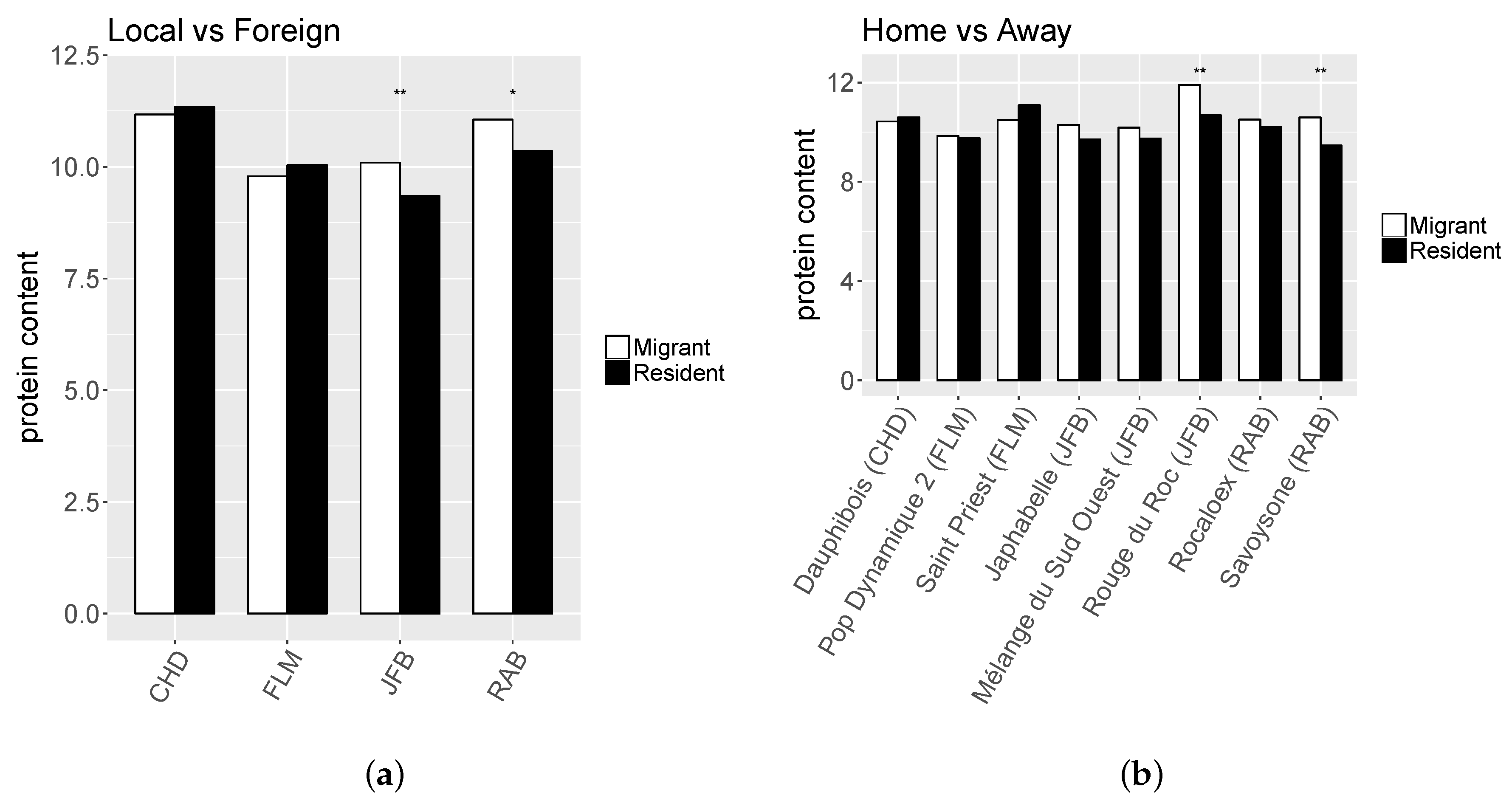
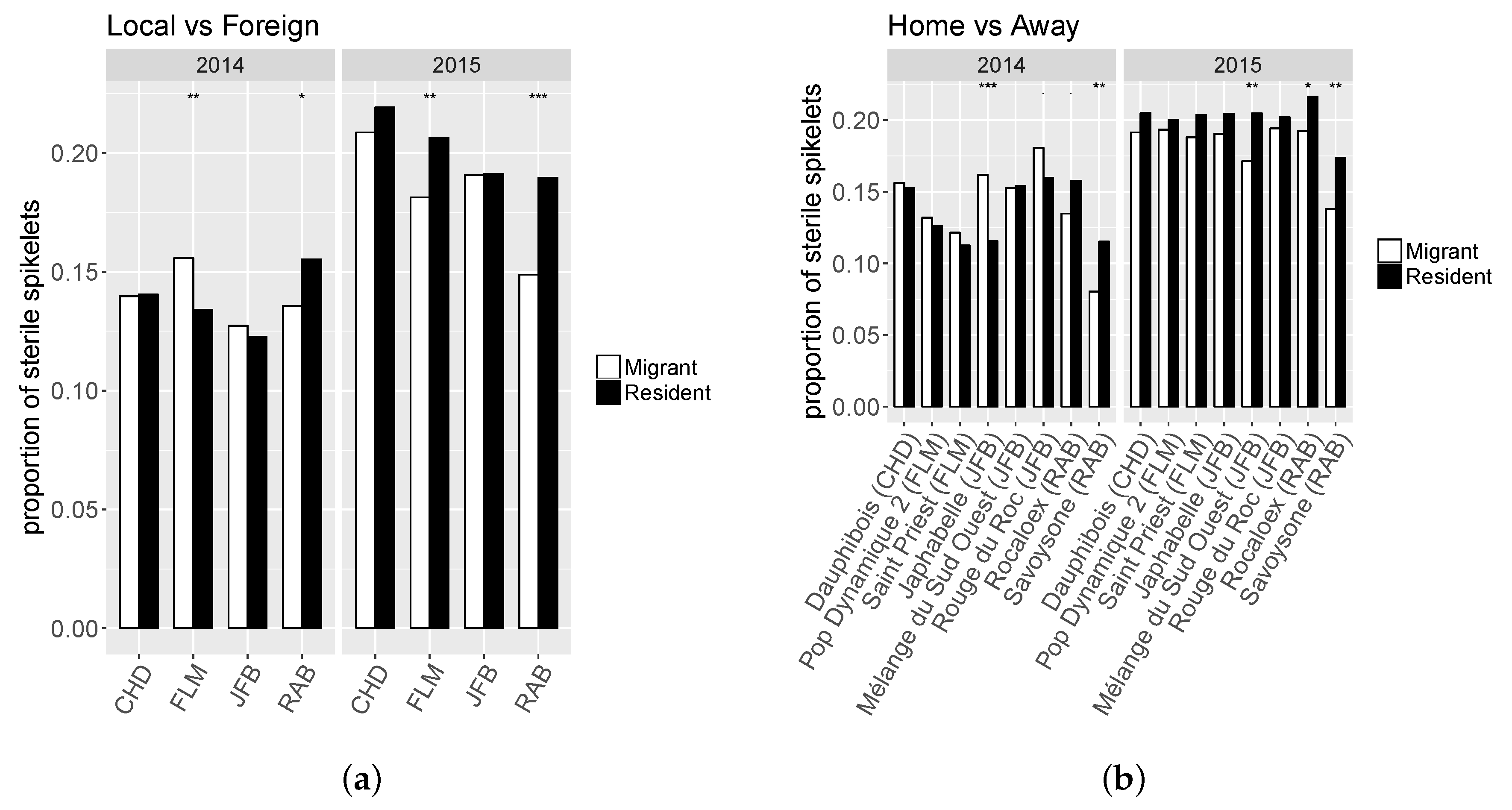
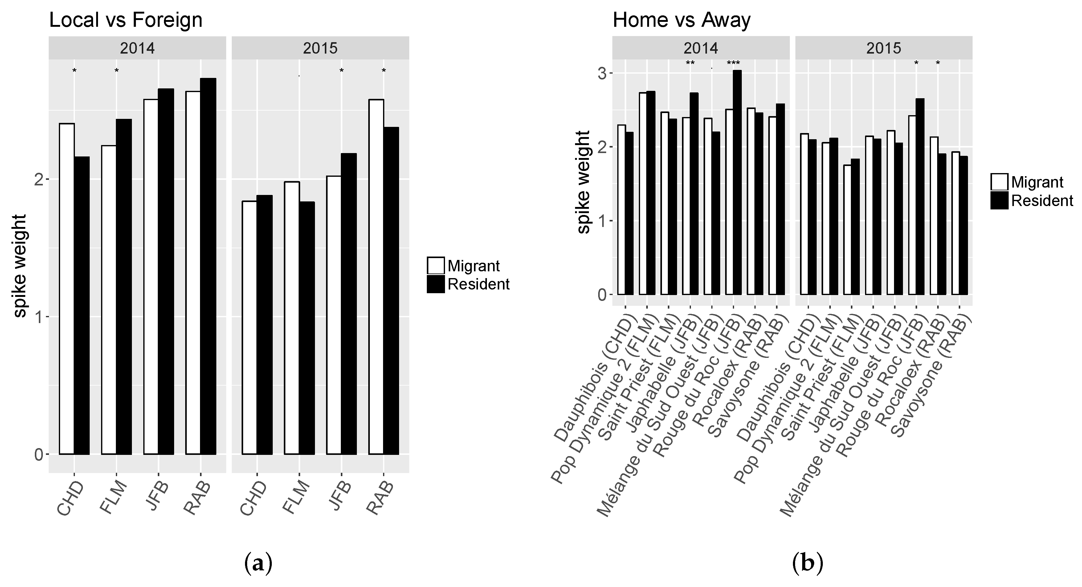
2.6.1. Local vs. Foreign
2.6.2. Home vs. Away
2.7. Temporal Stability
2.8. The Participatory Dimension
3. Results
3.1. Genetic Diversity
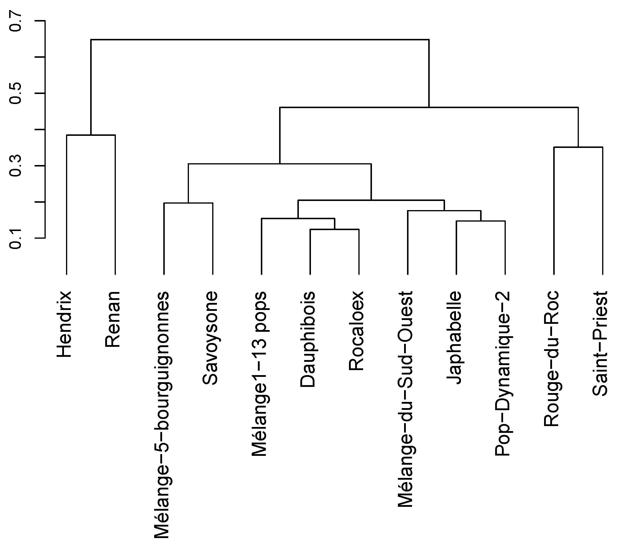
3.1.1. Genetic Distances between Varieties
3.1.2. Within-Variety Genetic Diversity
3.1.3. Correlations between Genetic Diversity and Phenotypic Variability
3.2. Local Adaptation
3.3. Spatio-Temporal Stability and Its Link with Genetic and Phenotypic Variability
3.3.1. Spatio-Temporal Stability
3.3.2. Correlations between Diversity and Stability
4. Discussion
4.1. Genetic and Phenotypic Diversity
4.2. Detection of Local Adaptation
4.3. Spatio-Temporal Stability of PPB Populations and Commercial Varieties
5. Conclusions
Supplementary Materials
Author Contributions
Funding
Acknowledgments
Conflicts of Interest
Abbreviations
| GY | grain yield |
| LLSD | last leaf to spike distance |
| TKW | thousand kernel weight |
| GN | number of grains per m |
| NSPK | number of spikelets per spike |
| PC | protein content |
| PH | plant height |
| PPB | Participatory Plant Breeding |
| NSPK_st | proportion of sterile kernels |
| SL | spike length |
| SW | spike weight |
Appendix A. Temporal Stability for Remaining Traits

| LLSD | SL | |||||||||||
|---|---|---|---|---|---|---|---|---|---|---|---|---|
| A | F | AF | Res | A | F | AF | Res | |||||
| Dauphibois | 0.112 | 0.205 | 0.152 | 0.252 | 0.065 | 0.041 | 0.075 | 0.171 | ||||
| Japhabelle | 0.089 | 0.166 | 0.180 | 0.223 | 0.083 | 0.056 | 0.061 | 0.154 | ||||
| Mélange-1 | 0.087 | 0.209 | 0.166 | 0.247 | 0.075 | 0.023 | 0.103 | 0.172 | ||||
| Mélange-5 | 0.195 | 0.185 | 0.176 | 0.240 | 0.078 | 0.049 | 0.055 | 0.145 | ||||
| Mélange-SO | 0.104 | 0.211 | 0.169 | 0.244 | 0.077 | 0.033 | 0.093 | 0.145 | ||||
| Pop-Dyn-2 | 0.000 | 0.132 | 0.195 | 0.266 | 0.106 | 0.052 | 0.057 | 0.146 | ||||
| Rocaloex | 0.133 | 0.239 | 0.144 | 0.237 | 0.080 | 0.039 | 0.071 | 0.182 | ||||
| Rouge-du-Roc | 0.152 | 0.170 | 0.195 | 0.162 | 0.048 | 0.000 | 0.096 | 0.143 | ||||
| Saint-Priest | 0.092 | 0.188 | 0.194 | 0.149 | 0.104 | 0.050 | 0.061 | 0.128 | ||||
| Savoysone | 0.180 | 0.241 | 0.144 | 0.176 | 0.133 | 0.000 | 0.099 | 0.149 | ||||
| Hendrix | 0.000 | 0.160 | 0.170 | 0.285 | 0.118 | 0.083 | 0.078 | 0.118 | ||||
| Renan | 0.000 | 0.196 | 0.214 | 0.256 | 0.063 | 0.000 | 0.108 | 0.148 | ||||
| Mean PPB | 0.114 | 0.195 | 0.172 | 0.220 | 0.085 | 0.034 | 0.077 | 0.154 | ||||
| Mean CV | 0.000 | 0.178 | 0.192 | 0.270 | 0.090 | 0.042 | 0.093 | 0.133 | ||||
| SW | NSPK | NSPK_st | ||||||||||
| A | F | AF | Res | A | F | AF | Res | A | F | AF | Res | |
| Dauphibois | 0.075 | 0.132 | 0.086 | 0.321 | 0.011 | 0.038 | 0.072 | 0.111 | 0.115 | 0.060 | 0.124 | 0.396 |
| Japhabelle | 0.156 | 0.102 | 0.091 | 0.305 | 0.030 | 0.073 | 0.045 | 0.116 | 0.180 | 0.000 | 0.106 | 0.385 |
| Mélange-1 | 0.108 | 0.142 | 0.140 | 0.312 | 0.000 | 0.070 | 0.073 | 0.114 | 0.184 | 0.036 | 0.172 | 0.386 |
| Mélange-5 | 0.129 | 0.143 | 0.111 | 0.277 | 0.000 | 0.084 | 0.069 | 0.116 | 0.138 | 0.000 | 0.074 | 0.386 |
| Mélange-SO | 0.091 | 0.138 | 0.127 | 0.295 | 0.022 | 0.058 | 0.069 | 0.116 | 0.147 | 0.083 | 0.117 | 0.395 |
| Pop-Dyn-2 | 0.194 | 0.163 | 0.052 | 0.287 | 0.044 | 0.050 | 0.068 | 0.106 | 0.200 | 0.039 | 0.114 | 0.374 |
| Rocaloex | 0.144 | 0.165 | 0.035 | 0.315 | 0.036 | 0.048 | 0.070 | 0.121 | 0.149 | 0.000 | 0.139 | 0.435 |
| Rouge-du-Roc | 0.082 | 0.152 | 0.123 | 0.301 | 0.041 | 0.000 | 0.089 | 0.089 | 0.115 | 0.016 | 0.120 | 0.333 |
| Saint-Priest | 0.219 | 0.180 | 0.049 | 0.267 | 0.043 | 0.049 | 0.053 | 0.075 | 0.246 | 0.000 | 0.143 | 0.402 |
| Savoysone | 0.222 | 0.192 | 0.060 | 0.265 | 0.032 | 0.071 | 0.072 | 0.098 | 0.327 | 0.000 | 0.222 | 0.557 |
| Hendrix | 0.155 | 0.140 | 0.086 | 0.323 | 0.014 | 0.055 | 0.067 | 0.092 | 0.259 | 0.127 | 0.143 | 0.359 |
| Renan | 0.135 | 0.167 | 0.143 | 0.298 | 0.041 | 0.012 | 0.092 | 0.102 | 0.131 | 0.000 | 0.261 | 0.465 |
| Mean PPB | 0.142 | 0.151 | 0.087 | 0.294 | 0.026 | 0.054 | 0.068 | 0.106 | 0.180 | 0.023 | 0.133 | 0.405 |
| Mean CV | 0.145 | 0.154 | 0.114 | 0.310 | 0.028 | 0.034 | 0.080 | 0.097 | 0.195 | 0.064 | 0.202 | 0.412 |
Appendix B. Markers Used for Genotyping
Appendix B.1. Markers in Neutral Zones
| Marker Name | Chr | Ref | Marker Name | Chr | Ref |
|---|---|---|---|---|---|
| wsnp_BE443995B_Ta_2_2 | 3A | 9K | wsnp_Ex_c11265_18216936 | 5B | 9K |
| wsnp_Ex_c1255_2411550 | 1A | 9K | wsnp_BE445506B_Ta_2_4 | 7B | 9K |
| wsnp_BE489326B_Ta_2_1 | 3B | 9K | wsnp_Ex_c18616_27481826 | 9K | |
| wsnp_Ex_c18800_27681277 | 7B | 9K | wsnp_Ex_c26312_35558700 | 5B | 9K |
| wsnp_Ex_c38105_45710671 | 5B | 9K | wsnp_Ex_c62701_62229607 | 5A | 9K |
| wsnp_Ex_c18965_27868480 | 6A | 9K | wsnp_Ex_c8588_14419007 | 1A | 9K |
| wsnp_Ex_c9502_15748469 | 6A | 9K | wsnp_Ex_c9763_16125630 | 6A | 9K |
| wsnp_Ex_rep_c102707_87814407 | 7B | 9K | wsnp_Ex_rep_c103087_88123733 | 1A | 9K |
| wsnp_BF484606A_TA_2_3 | 1A | 9K | wsnp_Ex_rep_c66389_64588992 | 1B | 9K |
| wsnp_Ex_rep_c70036_68988728 | 6B | 9K | wsnp_BG606986A_TA_2_4 | 1A | 9K |
| wsnp_JD_c19925_17854742 | 7A | 9K | wsnp_JD_c20555_18262260 | 7A | 9K |
| wsnp_BM136727B_Ta_2_6 | 6B | 9K | wsnp_BM140362A_Ta_2_2 | 1A | 9K |
| wsnp_BQ161779B_Ta_2_4 | 6B | 9K | BS00077147 | 7D | Kaspar db |
| wsnp_Ku_c3151_5892200 | 5B | 9K | BS00022478 | 2B | Kaspar db |
| wsnp_Ku_c3929_7189422 | 7A | 9K | BS00021865 | 2D | Kaspar db |
| wsnp_Ku_rep_c70220_69775367 | 5B | 9K | BS00060226 | 4A | Kaspar db |
| wsnp_Ku_rep_c73198_72796386 | 3B | 9K | BS00064002 | 4D | Kaspar db |
| wsnp_Ra_c107797_91270622 | 2A | 9K | BS00022277 | 5D | Kaspar db |
| wsnp_Ku_c13204_21105694 | 3D | 9K | BS00080040 | 6D | Kaspar db |
| wsnp_JG_c625_379570 | 5B | 9K | BS00096478 | 7D | Kaspar db |
| wsnp_Ku_c33335_42844594 | 3B | 9K | BS00026412 | 2B | Kaspar db |
| wsnp_Ku_c51039_56457361 | 5A | 9K | BS00023211 | 2D | Kaspar db |
| wsnp_Ku_rep_c72211_71920520 | 5B | 9K | BS00065607 | 4A | Kaspar db |
| wsnp_Ra_c1020_2062200 | 1D | 9K | BS00068103 | 4D | Kaspar db |
| wsnp_CAP12_c7952_3403722 | 5B | 9K | BS00085191 | 5D | Kaspar db |
| wsnp_Ra_c4254_7755493 | 6B | 9K | BS00087343 | 6D | Kaspar db |
Appendix B.2. Markers in Candidate Genes for Precocity
| Candidate Gene | Associated Trait | Chr | Polymorphism | Ref | Marker Name |
|---|---|---|---|---|---|
| PHYA | photoreceptors | 4A | SNP | 9K | wsnp_Ex_c1563_2987002 |
| ZTL | photoreceptors | 6B | SNP | 9K | wsnp_Ex_c18382_27210656 |
| VIL2 | vernalization | 6B | SNP | 9K | wsnp_Ex_c39304_46635517 |
| SMZ | photoperiod | 1B | SNP | 9K | wsnp_BE_403956B_Ta_2_3 |
| Vrn1B | vernalization | 1A | SNP | 9K | wsnp_Ex_c645_1273901 |
| Vrn1B | vernalization | 6A | SNP | 9K | wsnp_Ex_c7546_12900094 |
| SMZ | photoperiod | 1B | SNP | 9K | wsnp_Ex_c9063_15093396 |
| PHYA | photoreceptors | 4A | SNP | 9K | wsnp_Ex_rep_c66600_64897324 |
| C04 | photoperiod | 5B | SNP | 9K | wsnp_Ex_rep_c67690_66354931 |
| Vrn1B | vernalization | 6A | SNP | 9K | wsnp_Ex_rep_c69901_68864080 |
| CO1 | photoperiod | 7A | SNP | 9K | wsnp_JD_c15333_14824351 |
| TaHd1A | photoperiod | 5A | SNP | 9K | wsnp_Ku_c15816_24541712 |
| CO1 | photoperiod | 3B | SNP | 9K | wsnp_Ku_c48167_54427241 |
| SMZ | photoperiod | 4A | SNP | 9K | wsnp_CAP11_c3346_1639010 |
| SOC1 | photoperiod | 3A | SNP | 9K | wsnp_Ra_c16053_24607526 |
| C04 | photoperiod | 7A | SNP | 9K | wsnp_CAP12_c1461_744121 |
| ZTL | photoreceptors | 6B | SNP | 9K | wsnp_Ra_c3766_6947953 |
| Vrn1A | vernalization | 5A | SNP | [72] | |
| Vrn1A | vernalization | 5A | SNP | [72] | |
| Vrn1B | vernalization | 5B | SNP | [72] | |
| Vrn1B | vernalization | 5B | SNP | [72] | |
| Vrn1A | vernalization | 5A | SNP | [73] | |
| Vrn1B | vernalization | 5B | SNP | [74] | |
| Vrn3B | vernalization | 7B | SNP | [75] | |
| Vrn1B | vernalization | 5B | 6849bp indel | [72] | |
| TaGI3 | photoperiod | 3B | SNP | [76] | wsnp_Ex_rep_c67404_65986980 |
| LDDA | photoperiod | 5A | SNP | [76] | wsnp_Ku_c1102_2211433 |
| CO-B | photoperiod | 5B | SNP | [77] | |
| FTA | flowering | 7A | SSR | [78] | |
| Ppd-D1 | photoperiod | 2D | 2kb indel | [79] | |
| Vrn1A | vernalization | 5A | SNP | [73] | |
| Vrn1D | vernalization | 5D | 4kb indel | [72] | |
| TaGW2 | grain size | 6A | SNP | [80] | |
| Ppd-D1 | photoperiod | 2A | 305bp indel | [81] |
References
- Ray, D.K.; Gerber, J.S.; MacDonald, G.K.; West, P.C. Climate variation explains a third of global crop yield variability. Nat. Commun. 2015, 6. [Google Scholar] [CrossRef] [PubMed] [Green Version]
- Bren d’Amour, C.; Wenz, L.; Kalkuhl, M.; Christoph Steckel, J.; Creutzig, F. Teleconnected food supply shocks. Environ. Res. Lett. 2016, 11, 035007. [Google Scholar] [CrossRef]
- Liu, B.; Martre, P.; Ewert, F.; Porter, J.R.; Challinor, A.J.; Müller, C.; Ruane, A.C.; Waha, K.; Thorburn, P.J.; Aggarwal, P.K.; et al. Global wheat production with 1.5 and 2.0 °C above pre-industrial warming. Glob. Chang. Biol. 2018, 25, 1428–1444. [Google Scholar] [CrossRef] [PubMed]
- Trnka, M.; Rötter, R.P.; Ruiz-Ramos, M.; Kersebaum, K.C.; Olesen, J.E.; Žalud, Z.; Semenov, M.A. Adverse weather conditions for European wheat production will become more frequent with climate change. Nat. Clim. Chang. 2014, 4, 637–643. [Google Scholar] [CrossRef]
- Kahiluoto, H.; Kaseva, J.; Balek, J.; Olesen, J.E.; Ruiz-Ramos, M.; Gobin, A.; Kersebaum, K.C.; Takáč, J.; Ruget, F.; Ferrise, R.; et al. Decline in climate resilience of European wheat. Proc. Natl. Acad. Sci. USA 2019, 116, 123–128. [Google Scholar] [CrossRef] [PubMed] [Green Version]
- Frison, E.A.; Cherfas, J.; Hodgkin, T. Agricultural biodiversity is essential for a sustainable improvement in food and nutrition security. Sustainability 2011, 3, 238–253. [Google Scholar] [CrossRef] [Green Version]
- Abson, D.J.; Fraser, E.D.; Benton, T.G. Landscape diversity and the resilience of agricultural returns: A portfolio analysis of land-use patterns and economic returns from lowland agriculture. Agric. Food Secur. 2013, 2, 2. [Google Scholar] [CrossRef] [Green Version]
- Altieri, M.A. The ecological role of biodiversity in agroecosystems. Agric. Ecosyst. Environ. 1999, 74, 19–31. [Google Scholar] [CrossRef] [Green Version]
- Gaudin, A.C.M.; Tolhurst, T.N.; Ker, A.P.; Janovicek, K.; Tortora, C.; Martin, R.C.; Deen, W. Increasing crop diversity mitigates weather variations and improves yield stability. PLoS ONE 2015, 10, e0113261. [Google Scholar] [CrossRef] [Green Version]
- Renard, D.; Tilman, D. National food production stabilized by crop diversity. Nature 2019, 571, 257–260. [Google Scholar] [CrossRef]
- De Vallavieille-Pope, C. Management of disease resistance diversity of cultivars of a species in single fields: Controlling epidemics. Comptes Rendus Biol. 2004, 327, 611–620. [Google Scholar] [CrossRef] [PubMed]
- Mundt, C.C. Use of multiline cultivars and cultivar mixtures for disease management. Annu. Rev. Phytopathol. 2002, 40, 381–410. [Google Scholar] [CrossRef] [PubMed] [Green Version]
- Altieri, M.A.; Nicholls, C.I. The adaptation and mitigation potential of traditional agriculture in a changing climate. Clim. Chang. 2013, 140, 33–45. [Google Scholar] [CrossRef]
- Østergård, H.; Finckh, M.R.; Fontaine, L.; Goldringer, I.; Hoad, S.P.; Kristensen, K.; van Bueren, E.T.L.; Mascher, F.; Munk, L.; Wolfe, M.S. Time for a shift in crop production: Embracing complexity through diversity at all levels. J. Sci. Food Agric. 2009, 89, 1439–1445. [Google Scholar] [CrossRef]
- Finckh, M.; Gacek, E.; Goyeau, H.; Lannou, C.; Merz, U.; Mundt, C.; Munk, L.; Nadziak, J.; Newton, A.; de Vallavieille-Pope, C.; et al. Cereal variety and species mixtures in practice, with emphasis on disease resistance. Agronomie 2000, 20, 813–837. [Google Scholar] [CrossRef] [Green Version]
- Cardinale, B.J.; Matulich, K.L.; Hooper, D.U.; Byrnes, J.E.; Duffy, E.; Gamfeldt, L.; Balvanera, P.; O’Connor, M.I.; Gonzalez, A. The functional role of producer diversity in ecosystems. Am. J. Bot. 2011, 98, 572–592. [Google Scholar] [CrossRef] [Green Version]
- Cook-Patton, S.C.; McArt, S.H.; Parachnowitsch, A.L.; Thaler, J.S.; Agrawal, A.A. A direct comparison of the consequences of plant genotypic and species diversity on communities and ecosystem function. Ecology 2011, 92, 915–923. [Google Scholar] [CrossRef] [Green Version]
- Tilman, D.; Lehman, C.L.; Thomson, K.T. Plant diversity and ecosystem productivity: Theoretical considerations. Proc. Natl. Acad. Sci. USA 1997, 94, 1857–1861. [Google Scholar] [CrossRef] [Green Version]
- Goldringer, I.; Serpolay, E.; Rey, F.; Costanzo, A. Varieties and populations for on-farm participatory plant breeding. DIVERSIFOOD Innovation Factsheet 2. 2017. Available online: http://www.diversifood.eu/wp-content/uploads/2018/06/Diversifood_innovation_factsheet2_VarietiesPopulations.pdf (accessed on 2 January 2020).
- Reiss, E.R.; Drinkwater, L.E. Cultivar mixtures: A meta-analysis of the effect of intraspecific diversity on crop yield. Ecol. Appl. 2018, 28, 62–78. [Google Scholar] [CrossRef]
- Tomich, T.P.; Brodt, S.; Ferris, H.; Galt, R.; Horwath, W.R.; Kebreab, E.; Leveau, J.H.; Liptzin, D.; Lubell, M.; Merel, P.; et al. Agroecology: A review from a global-change perspective. Annu. Rev. Environ. Resour. 2011, 36, 193–222. [Google Scholar] [CrossRef] [Green Version]
- Barot, S.; Allard, V.; Cantarel, A.; Enjalbert, J.; Gauffreteau, A.; Goldringer, I.; Lata, J.C.; Le Roux, X.; Niboyet, A.; Porcher, E. Designing mixtures of varieties for multifunctional agriculture with the help of ecology. A review. Agron. Sustain. Dev. 2017, 37, 13. [Google Scholar] [CrossRef] [Green Version]
- Kiær, L.P.; Skovgaard, I.M.; Østergård, H. Grain yield increase in cereal variety mixtures: A meta-analysis of field trials. Field Crop. Res. 2009, 114, 361–373. [Google Scholar] [CrossRef]
- Prieto, I.; Violle, C.; Barre, P.; Durand, J.L.; Ghesquiere, M.; Litrico, I. Complementary effects of species and genetic diversity on productivity and stability of sown grasslands. Nat. Plants 2015, 1, 15033. [Google Scholar] [CrossRef] [PubMed]
- Helland, S.J.; Holland, J.B. Genome-wide genetic diversity among components does not cause cultivar blend responses. Crop Sci. 2003, 43, 1618–1627. [Google Scholar] [CrossRef] [Green Version]
- Houle, D. Comparing evolvability and variability of quantitative traits. Genetics 1992, 130, 195–204. [Google Scholar] [PubMed]
- Kawecki, T.J.; Ebert, D. Conceptual issues in local adaptation. Ecol. Lett. 2004, 7, 1225–1241. [Google Scholar] [CrossRef] [Green Version]
- Leimu, R.; Fischer, M. A meta-analysis of local adaptation in plants. PLoS ONE 2008, 3, e4010. [Google Scholar] [CrossRef] [Green Version]
- Linhart, Y.B.; Grant, M.C. Evolutionary significance of local genetic differentiation in plants. Annu. Rev. Ecol. Syst. 1996, 27, 237–277. [Google Scholar] [CrossRef]
- Galloway, L.F.; Fenster, C.B. Population differentiation in an annual legume: Local adaptation. Evolution 2000, 54, 1173–1181. [Google Scholar] [CrossRef]
- Blanquart, F.; Kaltz, O.; Nuismer, S.L.; Gandon, S. A practical guide to measuring local adaptation. Ecol. Lett. 2013, 16, 1195–1205. [Google Scholar] [CrossRef]
- Horneburg, B.; Becker, H.C. Crop adaptation in on-farm management by natural and conscious selection: A case study with lentil. Crop Sci. 2008, 48, 203–212. [Google Scholar] [CrossRef]
- Klaedtke, S.; Caproni, L.; Klauck, J.; de la Grandville, P.; Dutartre, M.; Stassart, P.; Chable, V.; Negri, V.; Raggi, L. Short-term local adaptation of historical common bean (Phaseolus vulgaris L.) varieties and implications for in situ management of bean diversity. Int. J. Mol. Sci. 2017, 18, 493. [Google Scholar] [CrossRef] [PubMed]
- Dawson, J.C.; Murphy, K.M.; Jones, S.S. Decentralized selection and participatory approaches in plant breeding for low-input systems. Euphytica 2008, 160, 143–154. [Google Scholar] [CrossRef]
- Ceccarelli, S. Wide adaptation: How wide? Euphytica 1989, 40, 197–205. [Google Scholar] [CrossRef]
- Desclaux, D.; Nolot, J.M.; Chiffoleau, Y.; Gozé, E.; Leclerc, C. Changes in the concept of genotype × environment interactions to fit agriculture diversification and decentralized participatory plant breeding: pluridisciplinary point of view. Euphytica 2008, 163, 533–546. [Google Scholar] [CrossRef]
- Witcombe, J.; Yadavendra, J. How much evidence is needed before client-oriented breeding (COB) is institutionalised? Evidence from rice and maize in India. Field Crop. Res. 2014, 167, 143–152. [Google Scholar] [CrossRef]
- Ceccarelli, S. Efficiency of Plant Breeding. Crop Sci. 2015, 55, 87–97. [Google Scholar] [CrossRef] [Green Version]
- Witcombe, J.R.; Joshi, A.; Goyal, S.N. Participatory plant breeding in maize: A case study from Gujarat, India. Euphytica 2003, 130, 413–422. [Google Scholar] [CrossRef]
- Rivière, P.; Pin, S.; Galic, N.; de Oliviera, Y.; David, O.; Dawson, J.; Wanner, A.; Heckmann, R.; Obbellianne, S.; Ronot, B.; et al. Mise en place d’une méthodologie de sélection participative sur le blé tendre en France. Innov. Agron. 2013, 32, 427–441. [Google Scholar]
- Rivière, P.; Dawson, J.C.; Goldringer, I.; David, O. Hierarchical Bayesian modeling for flexible experiments in decentralized participatory plant breeding. Crop Sci. 2015, 55, 1053–1067. [Google Scholar] [CrossRef]
- Van Frank, G.; Goldringer, I.; Rivière, P.; David, O. Influence of experimental design on decentralized, on-farm evaluation of populations: A simulation study. Euphytica 2019, 215, 126. [Google Scholar] [CrossRef]
- Borg, J.; Kiær, L.; Lecarpentier, C.; Goldringer, I.; Gauffreteau, A.; Saint-Jean, S.; Barot, S.; Enjalbert, J. Unfolding the potential of wheat cultivar mixtures: A meta-analysis perspective and identification of knowledge gaps. Field Crop. Res. 2017, 221, 298–313. [Google Scholar] [CrossRef]
- Creissen, H.E.; Jorgensen, T.H.; Brown, J.K.M. Increased yield stability of field-grown winter barley (Hordeum vulgare L.) varietal mixtures through ecological processes. Crop Prot. 2016, 85, 1–8. [Google Scholar] [CrossRef] [PubMed] [Green Version]
- Döring, T.F.; Annicchiarico, P.; Clarke, S.; Haigh, Z.; Jones, H.E.; Pearce, H.; Snape, J.; Zhan, J.; Wolfe, M.S. Comparative analysis of performance and stability among composite cross populations, variety mixtures and pure lines of winter wheat in organic and conventional cropping systems. Field Crop. Res. 2015, 183, 235–245. [Google Scholar] [CrossRef]
- Goldringer, I.; van Frank, G.; Bouvier d’Yvoire, C.; Forst, E.; Galic, N.; Garnault, M.; Locqueville, J.; Pin, S.; Bailly, J.; Baltassat, R.; et al. Agronomic evaluation of bread wheat varieties from participatory breeding: A combination of performance and robustness. Sustainability 2020, 12, 128. [Google Scholar] [CrossRef] [Green Version]
- LGC Biosearch Technologies. KASP Genotyping Chemistry. Available online: https://www.biosearchtech.com/products/pcr-kits-and-reagents/genotyping-assays/kasp-genotyping-chemistry (accessed on 13 August 2019).
- R Core Team. R: A Language and Environment for Statistical Computing; R Foundation for Statistical Computing: Vienna, Austria, 2018. [Google Scholar]
- Jombart, T.; Ahmed, I. Adegenet 1.3-1: New tools for the analysis of genome-wide SNP data. Bioinformatics 2011. [Google Scholar] [CrossRef] [Green Version]
- Nei, M. Analysis of gene diversity in subdivided populations. Proc. Natl. Acad. Sci. USA 1973, 70, 3321–3323. [Google Scholar] [CrossRef] [Green Version]
- Riviere, P.; van Frank, G.; David, O.; Muñoz, F.; Rouger, B.; Vindras, C.; Thomas, M.; Goldringer, I. PPBstats: An R Package to Perform Analysis Found within PPB Programmes Regarding Network of Seeds Circulation, Agronomic Trials, Organoleptic Tests and Molecular Experiments, version 0.25; 2019. Available online: https://github.com/priviere/PPBstats_web_site (accessed on 2 January 2020).
- Serpolay, E.; Dawson, J.C.; Chable, V.; Van Bueren, E.L.; Osman, A.; Pino, S.; Silveri, D.; Goldringer, I. Diversity of different farmer and modern wheat varieties cultivated in contrasting organic farming conditions in western Europe and implications for European seed and variety legislation. Org. Agric. 2011, 1, 127–145. [Google Scholar] [CrossRef]
- Ceccarelli, S.; Grando, S. Decentralized-participatory plant breeding: An example of demand driven research. Euphytica 2007, 155, 349–360. [Google Scholar] [CrossRef]
- Raggi, L.; Ceccarelli, S.; Negri, V. Evolution of a barley composite cross-derived population: An insight gained by molecular markers. J. Agric. Sci. 2016, 154, 23–39. [Google Scholar] [CrossRef]
- Enjalbert, J.; Dawson, J.C.; Paillard, S.; Rhoné, B.; Rousselle, Y.; Thomas, M.; Goldringer, I. Dynamic management of crop diversity: From an experimental approach to on-farm conservation. Comptes Rendus Biol. 2011, 334, 458–468. [Google Scholar] [CrossRef] [PubMed]
- Goldringer, I.; Enjalbert, J.; Raquin, A.L.; Brabant, P. Strong selection in wheat populations during ten generations of dynamic management. Genet. Sel. Evol. 2001, 33, S441–S463. [Google Scholar] [CrossRef]
- Goldringer, I.; Prouin, C.; Rousset, M.; Galic, N.; Bonnin, I. Rapid differentiation of experimental populations of wheat for heading time in response to local climatic conditions. Ann. Bot. 2006, 98, 805–817. [Google Scholar] [CrossRef] [PubMed] [Green Version]
- Thomas, M.; Thépot, S.; Galic, N.; Jouanne-Pin, S.; Remoué, C.; Goldringer, I. Diversifying mechanisms in the on-farm evolution of crop mixtures. Mol. Ecol. 2015, 24, 2937–2954. [Google Scholar] [CrossRef] [PubMed] [Green Version]
- Rhoné, B.; Vitalis, R.; Goldringer, I.; Bonnin, I. Evolution of flowering time in experimental wheat populations: A comprehensive approach to detect genetic signatures of natural selection. Evolution 2010, 64, 2110–2125. [Google Scholar] [CrossRef] [PubMed]
- Becker, U.; Colling, G.; Dostal, P.; Jakobsson, A.; Matthies, D. Local adaptation in the monocarpic perennial Carlina vulgaris at different spatial scales across Europe. Oecologia 2006, 150, 506–518. [Google Scholar] [CrossRef]
- Dawson, J.C.; Serpolay, E.; Giuliano, S.; Schermann, N.; Galic, N.; Berthellot, J.F.; Chesneau, V.; Ferté, H.; Mercier, F.; Osman, A.; et al. Phenotypic diversity and evolution of farmer varieties of bread wheat on organic farms in Europe. Genet. Resour. Crop Evol. 2013, 60, 145–163. [Google Scholar] [CrossRef]
- Crispo, E. Modifying effects of phenotypic plasticity on interactions among natural selection, adaptation and gene flow. J. Evol. Biol. 2008, 21, 1460–1469. [Google Scholar] [CrossRef]
- Dawson, J.C.; Rivière, P.; Berthellot, J.F.; Mercier, F.; Kochko, P.d.; Galic, N.; Pin, S.; Serpolay, E.; Thomas, M.; Giuliano, S.; et al. Collaborative plant breeding for organic agricultural systems in developed countries. Sustainability 2011, 3, 1206–1223. [Google Scholar] [CrossRef] [Green Version]
- Magnard, A. Mélanger les variétés de blé, une pratique qui monte. Fr. Agric. 2017, 3724, 37. [Google Scholar]
- FranceAgriMer. Variétés et rendements des céréales biologiques. Récolte 2015; FranceAgriMer: Montreuil, France, 2016. [Google Scholar]
- Raggi, L.; Ciancaleoni, S.; Torricelli, R.; Terzi, V.; Ceccarelli, S.; Negri, V. Evolutionary breeding for sustainable agriculture: Selection and multi-environmental evaluation of barley populations and lines. Field Crop. Res. 2017, 204, 76–88. [Google Scholar] [CrossRef]
- Creissen, H.E.; Jorgensen, T.H.; Brown, J.K.M. Stabilization of yield in plant genotype mixtures through compensation rather than complementation. Ann. Bot. 2013, 112, 1439–1447. [Google Scholar] [CrossRef] [PubMed] [Green Version]
- Kloppenburg, J. Impeding dispossession, enabling repossession: Biological open source and the recovery of seed sovereignty. J. Agrar. Chang. 2010, 10, 367–388. [Google Scholar] [CrossRef]
- Stassart, P.M.; Baret, P.; Grégoire, J.C.; Hance, T. L’agroécologie: Trajectoire et potentiel pour une transition vers des systèmes alimentaires durables. In Agroécologie entre pratiques et sciences sociales, Educagri Editions; Dam, D.V., Streith, M., Nizet, J., Stassart, P.M., Eds.; Educagri: Dijon, France, 2012; pp. 25–51. [Google Scholar]
- Wolfe, M.S.; Brandle, U.; Koller, B.; Limpert, E.; McDermott, J.M.; Miiller, K.; Schaffner, D. Barley mildew in Europe: Population biology and host resistance. Euphytica 1992, 63, 125–139. [Google Scholar] [CrossRef]
- Cavanagh, C.R.; Chao, S.; Wang, S.; Huang, B.E.; Stephen, S.; Kiani, S.; Forrest, K.; Saintenac, C.; Brown-Guedira, G.L.; Akhunova, A.; et al. Genome-wide comparative diversity uncovers multiple targets of selection for improvement in hexaploid wheat landraces and cultivars. Proc. Natl. Acad. Sci. USA 2013, 110, 8057–8062. [Google Scholar] [CrossRef] [PubMed] [Green Version]
- Fu, D.; Szűcs, P.; Yan, L.; Helguera, M.; Skinner, J.S.; von Zitzewitz, J.; Hayes, P.M.; Dubcovsky, J. Large deletions within the first intron in VRN-1 are associated with spring growth habit in barley and wheat. Mol. Genet. Genom. 2005, 273, 54–65. [Google Scholar] [CrossRef] [Green Version]
- Sherman, J.D.; Yan, L.; Talbert, L.; Dubcovsky, J. A PCR marker for growth habit in common wheat based on allelic variation at the VRN-A1 gene. Crop Sci. 2004, 44, 1832–1838. [Google Scholar] [CrossRef]
- Shcherban, A.B.; Efremova, T.T.; Salina, E.A. Identification of a new Vrn-B1 allele using two near-isogenic wheat lines with difference in heading time. Mol. Breed. 2012, 29, 675–685. [Google Scholar] [CrossRef]
- Yan, L.; Fu, D.; Li, C.; Blechl, A.; Tranquilli, G.; Bonafede, M.; Sanchez, A.; Valarik, M.; Yasuda, S.; Dubcovsky, J. The wheat and barley vernalization gene VRN3 is an orthologue of FT. Proc. Natl. Acad. Sci. USA 2006, 103, 19581–19586. [Google Scholar] [CrossRef] [Green Version]
- Rhoné, B. Etude des mécanismes génétiques impliqués dans l’adaptation climatique de populations expérimentales de blé tendre. Ph.D. Thesis, AgroParisTech, Paris, France, 2008. [Google Scholar]
- Rhoné, B.; Remoué, C.; Galic, N.; Goldringer, I.; Bonnin, I. Insight into the genetic bases of climatic adaptation in experimentally evolving wheat populations. Mol. Ecol. 2008, 17, 930–943. [Google Scholar] [CrossRef]
- Bonnin, I.; Rousset, M.; Madur, D.; Sourdille, P.; Dupuits, C.; Brunel, D.; Goldringer, I. FT genome A and D polymorphisms are associated with the variation of earliness components in hexaploid wheat. Theor. Appl. Genet. 2008, 116, 383–394. [Google Scholar] [CrossRef] [PubMed]
- Beales, J.; Turner, A.; Griffiths, S.; Snape, J.W.; Laurie, D.A. A Pseudo-Response Regulator is misexpressed in the photoperiod insensitive Ppd-D1a mutant of wheat (Triticum aestivum L.). Theor. Appl. Genet. 2007, 115, 721–733. [Google Scholar] [CrossRef] [PubMed]
- Su, Z.; Hao, C.; Wang, L.; Dong, Y.; Zhang, X. Identification and development of a functional marker of TaGW2 associated with grain weight in bread wheat (Triticum aestivum L.). Theor. Appl. Genet. 2011, 122, 211–223. [Google Scholar] [CrossRef] [PubMed]
- Wilhelm, E.P.; Turner, A.S.; Laurie, D.A. Photoperiod insensitive PPd-A1a mutations in tetraploid wheat (Triticum durum Desf.). Theor. Appl. Genet. 2009, 118, 285–294. [Google Scholar] [CrossRef]
- Akhunov, E.D.; Akhunova, A.R.; Anderson, O.D.; Anderson, J.A.; Blake, N.; Clegg, M.T.; Coleman-Derr, D.; Conley, E.J.; Crossman, C.C.; Deal, K.R.; et al. Nucleotide diversity maps reveal variation in diversity among wheat genomes and chromosomes. BMC Genom. 2010, 11, 702. [Google Scholar] [CrossRef] [Green Version]
- Chao, S.; Dubcovsky, J.; Dvorak, J.; Luo, M.C.; Baenziger, S.P.; Matnyazov, R.; Clark, D.R.; Talbert, L.E.; Anderson, J.A.; Dreisigacker, S.; et al. Population- and genome-specific patterns of linkage disequilibrium and SNP variation in spring and winter wheat (Triticum aestivum L.). BMC Genom. 2010, 11, 727. [Google Scholar] [CrossRef] [Green Version]
- Higgins, J.A.; Bailey, P.C.; Laurie, D.A. Comparative genomics of flowering time pathways using Brachypodium distachyon as a model for the temperate grasses. PLoS ONE 2010, 5, e10065. [Google Scholar] [CrossRef]


| Variety | Farmer | Development Process | Creation Date | Evaluated in Their Farm of Origin |
|---|---|---|---|---|
| Saint-Priest | FLM | Derived from a Swedish variety (Progress) | 2004 | X |
| Rouge du Roc | JFB | Population derived from a mass selection within a landrace | 2001 | X |
| Savoysone | RAB | Population derived from a cross between two landraces | 2010 | X |
| Pop dynamique 2 | FLM | Mixture of 3 landraces and 2 recent varieties | 2010 | X |
| Mélange du Sud-Ouest | JFB | Mixture of about 18 landraces | early 2000 | X |
| Rocaloex | RAB | Mixture of 11 crosses | 2012 | X |
| Japhabelle | JFB | Mixture of 25 crosses | 2009 | X |
| Dauphibois | CHD | Mixture of 26 landraces and crosses | 2012 | X |
| Mélange 5 bourguignonnes | BER | Mixture of 11 landraces | 2012 | |
| Mélange1 13 pops | BER | Mixture of 13 crosses | 2012 | |
| Renan | INRA | Commercial pure line registered in 1989 | ||
| Hendrix | INRA | Commercial pure line registered in 2013 |
| Farm | Growing Season | Soil Type | Sowing Date | Sowing Density | Plot Size |
|---|---|---|---|---|---|
| CHD | 2013–2014 | Clay-limestone | 13 November 2013 | 300 grains/m | 22.5 m |
| CHD | 2014–2015 | Clay-limestone | 29 October 2014 | 300 grains/m | 10 m |
| FLM | 2013–2014 | Sandy hydromorphic | 27 November 2013 | 300 grains/m | 10 m |
| FLM | 2014–2015 | Sandy hydromorphic | November 2014 | 300 grains/m | 10 m |
| FRC | 2013–2014 | Clay-limestone dry | 1 November 2013 | 23 g/m | 10 m |
| FRC | 2014–2015 | Clay-limestone dry | 18 December 2014 | 250 grains/m2 | 10 m |
| JFB | 2013–2014 | Clay-limestone | 12 December 2013 | 12.5 g/m | 8 m |
| JFB | 2014–2015 | Clay-limestone | 13 November 2014 | 10 m | |
| JSG | 2013–2014 | Clay-limestone | 27 November 2013 | 350 grains/m | 7 m |
| JSG | 2014–2015 | Clay-limestone | 31 October 2014 | 350 grains/m | 7.8 m |
| RAB | 2013–2014 | Loam | 2 November 2013 | 20 g/m | 22.5 m |
| RAB | 2014–2015 | Clay-loam | 29 October 2014 | 15 g/m | 120 m |
| Population | Number of Individuals | He | Ho | ||
|---|---|---|---|---|---|
| NE | CA | NE | CA | ||
| Renan | 30 | 0.000 | 0.000 | - | - |
| Hendrix | 29 | 0.004 | 0.000 | 0.000 | 0.000 |
| Rouge-du-Roc | 90 | 0.084 | 0.062 | 0.001 | 0.000 |
| Saint-Priest | 90 | 0.129 | 0.081 | 0.005 | 0.007 |
| Mélange-5-bourguignonnes | 90 | 0.283 | 0.128 | 0.010 | 0.004 |
| Savoysone | 90 | 0.290 | 0.109 | 0.011 | 0.010 |
| Pop-Dynamique-2 | 90 | 0.361 | 0.205 | 0.006 | 0.006 |
| Mélange-du-Sud-Ouest | 90 | 0.363 | 0.233 | 0.010 | 0.009 |
| Rocaloex | 90 | 0.377 | 0.157 | 0.002 | 0.001 |
| Japhabelle | 90 | 0.388 | 0.146 | 0.008 | 0.004 |
| Mélange1-13 pops | 90 | 0.396 | 0.150 | 0.007 | 0.002 |
| Dauphibois | 90 | 0.402 | 0.198 | 0.004 | 0.002 |
| NE | CA | |
|---|---|---|
| PH | 0.862 | 0.815 |
| LLSD | 0.832 | 0.891 |
| awns | 0.876 | 0.869 |
| color | 0.865 | 0.773 |
| curve | 0.556 | 0.507 |
| SL | 0.717 | 0.580 |
| SW | −0.243 | −0.235 |
| NSPK | 0.814 | 0.716 |
| NSPK_st | 0.355 | 0.203 |
| SL | SW | NSPK | NSPK_st | |||||||||
|---|---|---|---|---|---|---|---|---|---|---|---|---|
| Df | SS | F | Df | SS | F | Df | SS | F | Df | SS | F | |
| farm | 3 | 75,850.5 | 111.42 *** | 3 | 116.3 | 97.89 *** | 3 | 2085.3 | 151.19 *** | 3 | 0.3 | 23.15 *** |
| pop | 7 | 35,836.1 | 22.56 *** | 7 | 50.9 | 18.36 *** | 7 | 1849.9 | 57.48 *** | 7 | 1.2 | 39.48 *** |
| year | 1 | 66,707.2 | 293.96 *** | 1 | 113.5 | 286.65 *** | 1 | 8.3 | 1.81 | 1 | 1.8 | 405.72 *** |
| MR | 1 | 297 | 1.31 | 1 | 0.1 | 0.23 | 1 | 8.3 | 1.82 | 1 | 0 | 9.56 ** |
| farm × year | 3 | 69,552.6 | 102.17 *** | 3 | 20.3 | 17.11 *** | 3 | 357.1 | 25.89 *** | 3 | 0.4 | 26.91 *** |
| farm × MR | 3 | 2578.8 | 3.79 * | 3 | 2.6 | 2.16 | 3 | 13.4 | 0.97 | 3 | 0.1 | 4.8 ** |
| rep/farm × year | 8 | 18,186.1 | 10.02 *** | 8 | 21.1 | 6.67 *** | 8 | 165.6 | 4.5 *** | 8 | 0.2 | 6.29 *** |
| farm × year × MR | 4 | 3718.8 | 4.1 ** | 4 | 9.6 | 6.05 *** | 4 | 26 | 1.42 | 4 | 0.1 | 5.87 *** |
| Residuals | 3100 | 703,478.4 | 3080 | 1219.4 | 3080 | 14,160.1 | 3076 | 13.4 | ||||
| TKW | PC | GN | GY | |||||||||
| Df | SS | F | Df | SS | F | Df | SS | F | Df | SS | F | |
| farm | 3 | 189.8 | 15.81 *** | 3 | 48.9 | 44.85 *** | 3 | 2,218,503.5 | 92.06 *** | 3 | 5485.3 | 96.82 *** |
| pop | 7 | 604.7 | 21.58 *** | 7 | 31.6 | 12.42 *** | 7 | 39,4951.2 | 7.02 *** | 7 | 400.6 | 3.03 ** |
| year | 1 | 158.1 | 39.5 *** | 1 | 152.4 | 419.4 *** | 1 | 252,074.2 | 31.38 *** | 1 | 870.7 | 46.11 *** |
| MR | 1 | 5.7 | 1.42 | 1 | 2.8 | 7.58 ** | 1 | 177.3 | 0.02 | 1 | 0.4 | 0.02 |
| farm × year | 3 | 100 | 8.32 *** | 3 | 82.5 | 75.66 *** | 3 | 1,214,761.2 | 50.41 *** | 3 | 2717.9 | 47.97 *** |
| farm × MR | 3 | 3 | 0.25 | 3 | 3.3 | 3.06 * | 3 | 47,465.2 | 1.97 | 3 | 95.4 | 1.68 |
| rep/farm × year | 8 | 59.8 | 1.87 | 8 | 4.3 | 1.48 | 8 | 165,843.4 | 2.58 * | 8 | 249 | 1.65 |
| farm × year × MR | 4 | 14.2 | 0.89 | 4 | 1.2 | 0.82 | 4 | 49,122.2 | 1.53 | 4 | 81.3 | 1.08 |
| Residuals | 95 | 380.4 | 94 | 34.2 | 89 | 714,887.2 | 89 | 1680.7 | ||||
| SL | SW | NSPK | NSPK_st | |||||||||
|---|---|---|---|---|---|---|---|---|---|---|---|---|
| Df | SS | F | Df | SS | F | Df | SS | F | Df | SS | F | |
| farm | 3 | 75,850.5 | 112.65 *** | 3 | 116.3 | 101.03 *** | 3 | 2085.3 | 151.94 *** | 3 | 0.3 | 23.52 *** |
| pop | 7 | 35,836.1 | 22.81 *** | 7 | 50.9 | 18.95 *** | 7 | 1849.9 | 57.77 *** | 7 | 1.2 | 40.1 *** |
| year | 1 | 66,707.2 | 297.21 *** | 1 | 113.5 | 295.84 *** | 1 | 8.3 | 1.81 | 1 | 1.8 | 412.1 *** |
| MR | 1 | 297 | 1.32 | 1 | 0.1 | 0.24 | 1 | 8.3 | 1.82 | 1 | 0 | 9.71 ** |
| farm × year | 3 | 69,552.6 | 103.29 *** | 3 | 20.3 | 17.66 *** | 3 | 357.1 | 26.02 *** | 3 | 0.4 | 27.33 *** |
| pop × MR | 7 | 5048.4 | 3.21 ** | 7 | 15.4 | 5.72 *** | 7 | 59.7 | 1.86 | 7 | 0.1 | 3.78 *** |
| rep/farm × year | 8 | 18,223.1 | 10.15 *** | 8 | 21.1 | 6.89 *** | 8 | 165.4 | 4.52 *** | 8 | 0.2 | 6.38 *** |
| pop × year × MR | 15 | 12,269.9 | 3.64 *** | 15 | 40.4 | 7.02 *** | 15 | 118.5 | 1.73 * | 15 | 0.3 | 5.03 *** |
| Residuals | 3085 | 692,420.7 | 3065 | 1175.8 | 3065 | 14,021.4 | 3061 | 13.1 | ||||
| TKW | PC | GN | GY | |||||||||
| Df | SS | F | Df | SS | F | Df | SS | F | Df | SS | F | |
| farm | 3 | 189.8 | 17.85 *** | 3 | 48.9 | 45.27 *** | 3 | 2,218,503.5 | 96.92 *** | 3 | 5485.3 | 111.27 *** |
| pop | 7 | 604.7 | 24.37 *** | 7 | 31.6 | 12.54 *** | 7 | 394,951.2 | 7.39 *** | 7 | 400.6 | 3.48 ** |
| year | 1 | 158.1 | 44.61 *** | 1 | 152.4 | 423.35 *** | 1 | 252,074.2 | 33.04 *** | 1 | 870.7 | 52.98 *** |
| MR | 1 | 5.7 | 1.61 | 1 | 2.8 | 7.65 ** | 1 | 177.3 | 0.02 | 1 | 0.4 | 0.02 |
| farm × year | 3 | 100 | 9.4 *** | 3 | 82.5 | 76.38 *** | 3 | 1,214,761.2 | 53.07 *** | 3 | 2717.9 | 55.13 *** |
| pop × MR | 7 | 7.8 | 0.31 | 7 | 6.2 | 2.47 * | 7 | 70,444.7 | 1.32 | 7 | 170.9 | 1.49 |
| rep/farm × year | 8 | 59.8 | 2.11 * | 8 | 4.3 | 1.5 | 8 | 166,093.2 | 2.72 * | 8 | 248.9 | 1.89 |
| pop × year × MR | 15 | 106.2 | 2 * | 15 | 4 | 0.75 | 15 | 176,163.7 | 1.54 | 15 | 470.7 | 1.91 * |
| Residuals | 80 | 283.6 | 79 | 28.4 | 74 | 564,616.3 | 74 | 1216 | ||||
| PH | TKW | |||||||||||
|---|---|---|---|---|---|---|---|---|---|---|---|---|
| Y | F | FY | Res | Y | F | FY | Res | |||||
| Dauphibois | 0.000 | 0.140 | 0.100 | 0.099 | 0.031 | 0.042 | 0.062 | 0.042 | ||||
| Japhabelle | 0.000 | 0.139 | 0.101 | 0.087 | 0.000 | 0.043 | 0.063 | 0.031 | ||||
| Mélange-1 | 0.000 | 0.148 | 0.118 | 0.089 | 0.000 | 0.065 | 0.065 | 0.031 | ||||
| Mélange-5 | 0.044 | 0.173 | 0.090 | 0.082 | 0.012 | 0.076 | 0.053 | 0.034 | ||||
| Mélange-SO | 0.000 | 0.148 | 0.121 | 0.086 | 0.025 | 0.075 | 0.038 | 0.039 | ||||
| Pop-Dyn-2 | 0.000 | 0.131 | 0.093 | 0.076 | 0.003 | 0.085 | 0.000 | 0.034 | ||||
| Rocaloex | 0.000 | 0.150 | 0.086 | 0.091 | 0.006 | 0.066 | 0.046 | 0.032 | ||||
| Rouge-du-Roc | 0.000 | 0.143 | 0.127 | 0.074 | 0.000 | 0.060 | 0.050 | 0.060 | ||||
| Saint-Priest | 0.018 | 0.137 | 0.081 | 0.072 | 0.011 | 0.073 | 0.019 | 0.036 | ||||
| Savoysone | 0.037 | 0.147 | 0.112 | 0.078 | 0.000 | 0.083 | 0.016 | 0.036 | ||||
| Hendrix | 0.000 | 0.138 | 0.125 | 0.075 | 0.000 | 0.055 | 0.068 | 0.041 | ||||
| Renan | 0.000 | 0.119 | 0.140 | 0.083 | 0.000 | 0.059 | 0.035 | 0.031 | ||||
| Mean PPB | 0.010 | 0.146 | 0.103 | 0.083 | 0.009 | 0.067 | 0.041 | 0.038 | ||||
| Mean CV | 0.000 | 0.128 | 0.132 | 0.079 | 0.000 | 0.057 | 0.052 | 0.036 | ||||
| PC | GN | GY | ||||||||||
| Y | F | FY | Res | Y | F | FY | Res | Y | F | FY | Res | |
| Dauphibois | 0.155 | 0.069 | 0.097 | 0.072 | 0.000 | 0.228 | 0.234 | 0.115 | 0.000 | 0.223 | 0.236 | 0.133 |
| Japhabelle | 0.142 | 0.000 | 0.105 | 0.053 | 0.000 | 0.217 | 0.292 | 0.173 | 0.000 | 0.204 | 0.326 | 0.162 |
| Mélange-1 | 0.120 | 0.000 | 0.103 | 0.040 | 0.134 | 0.221 | 0.196 | 0.246 | 0.152 | 0.208 | 0.242 | 0.258 |
| Mélange-5 | 0.101 | 0.000 | 0.100 | 0.061 | 0.000 | 0.264 | 0.146 | 0.212 | 0.063 | 0.286 | 0.162 | 0.207 |
| Mélange-SO | 0.173 | 0.000 | 0.089 | 0.081 | 0.000 | 0.240 | 0.234 | 0.139 | 0.000 | 0.235 | 0.255 | 0.113 |
| Pop-Dyn-2 | 0.088 | 0.000 | 0.096 | 0.076 | 0.000 | 0.149 | 0.343 | 0.176 | 0.000 | 0.216 | 0.343 | 0.175 |
| Rocaloex | 0.162 | 0.000 | 0.100 | 0.054 | 0.000 | 0.198 | 0.307 | 0.125 | 0.000 | 0.205 | 0.308 | 0.113 |
| Rouge-du-Roc | 0.139 | 0.051 | 0.096 | 0.065 | 0.000 | 0.270 | 0.225 | 0.286 | 0.000 | 0.266 | 0.226 | 0.243 |
| Saint-Priest | 0.135 | 0.000 | 0.095 | 0.053 | 0.000 | 0.149 | 0.229 | 0.170 | 0.000 | 0.183 | 0.272 | 0.150 |
| Savoysone | 0.174 | 0.000 | 0.113 | 0.052 | 0.000 | 0.247 | 0.222 | 0.134 | 0.000 | 0.257 | 0.246 | 0.142 |
| Hendrix | 0.249 | 0.000 | 0.123 | 0.058 | 0.000 | 0.331 | 0.382 | 0.266 | 0.000 | 0.337 | 0.404 | 0.261 |
| Renan | 0.247 | 0.000 | 0.073 | 0.047 | 0.000 | 0.404 | 0.279 | 0.271 | 0.000 | 0.395 | 0.302 | 0.254 |
| Mean PPB | 0.139 | 0.012 | 0.099 | 0.061 | 0.013 | 0.218 | 0.243 | 0.178 | 0.022 | 0.228 | 0.262 | 0.170 |
| Mean CV | 0.248 | 0.000 | 0.098 | 0.052 | 0.000 | 0.368 | 0.330 | 0.268 | 0.000 | 0.366 | 0.353 | 0.258 |
| Temporal | Spatial | |||||
|---|---|---|---|---|---|---|
| Diversity | Variety Effect | Diversity | Variety Effect | |||
| NE | CA | NE | CA | |||
| PH | 0.455 | 0.487 | 0.233 | −0.408 | −0.337 | −0.568 |
| LLSD | −0.185 | −0.147 | −0.770 | −0.270 | −0.143 | −0.242 |
| SL | 0.222 | 0.287 | 0.135 | −0.049 | −0.069 | 0.503 |
| SW | 0.374 | 0.444 | 0.136 | 0.302 | 0.260 | 0.153 |
| NSPK | 0.480 | 0.361 | 0.475 | −0.578 | −0.426 | −0.342 |
| NSPK_st | 0.300 | 0.427 | 0.775 | 0.135 | −0.033 | −0.290 |
| TKW | −0.182 | −0.124 | −0.062 | −0.068 | −0.187 | 0.194 |
| PC | 0.582 | 0.632 | 0.384 | −0.033 | −0.111 | −0.425 |
| GN | 0.072 | 0.140 | −0.581 | 0.646 | 0.678 | −0.152 |
| GY | 0.060 | 0.190 | −0.537 | 0.730 | 0.711 | −0.435 |
© 2020 by the authors. Licensee MDPI, Basel, Switzerland. This article is an open access article distributed under the terms and conditions of the Creative Commons Attribution (CC BY) license (http://creativecommons.org/licenses/by/4.0/).
Share and Cite
van Frank, G.; Rivière, P.; Pin, S.; Baltassat, R.; Berthellot, J.-F.; Caizergues, F.; Dalmasso, C.; Gascuel, J.-S.; Hyacinthe, A.; Mercier, F.; et al. Genetic Diversity and Stability of Performance of Wheat Population Varieties Developed by Participatory Breeding. Sustainability 2020, 12, 384. https://doi.org/10.3390/su12010384
van Frank G, Rivière P, Pin S, Baltassat R, Berthellot J-F, Caizergues F, Dalmasso C, Gascuel J-S, Hyacinthe A, Mercier F, et al. Genetic Diversity and Stability of Performance of Wheat Population Varieties Developed by Participatory Breeding. Sustainability. 2020; 12(1):384. https://doi.org/10.3390/su12010384
Chicago/Turabian Stylevan Frank, Gaëlle, Pierre Rivière, Sophie Pin, Raphaël Baltassat, Jean-François Berthellot, François Caizergues, Christian Dalmasso, Jean-Sébastien Gascuel, Alexandre Hyacinthe, Florent Mercier, and et al. 2020. "Genetic Diversity and Stability of Performance of Wheat Population Varieties Developed by Participatory Breeding" Sustainability 12, no. 1: 384. https://doi.org/10.3390/su12010384
APA Stylevan Frank, G., Rivière, P., Pin, S., Baltassat, R., Berthellot, J.-F., Caizergues, F., Dalmasso, C., Gascuel, J.-S., Hyacinthe, A., Mercier, F., Montaz, H., Ronot, B., & Goldringer, I. (2020). Genetic Diversity and Stability of Performance of Wheat Population Varieties Developed by Participatory Breeding. Sustainability, 12(1), 384. https://doi.org/10.3390/su12010384