A Markov Regime Switching Approach towards Assessing Resilience of Romanian Collective Investment Undertakings


Abstract
1. Introduction
2. Literature Review
3. Data and Methods
3.1. Sample
- BET Index of the Bucharest Stock Exchange price index
- Stoxx 600 Index price index
- the yield for the Romanian sovereign bond market with 5 years maturity (ROMGGR05 Index)
- the yield for the German/EUR sovereign bond market with 5 years maturity (GTEUR5YR Corp)
- the EUR/RON exchange rate
3.2. Research Methodology
- Stage 1: Initial data preparation
- Stage 2: Computing daily conditional volatilities
- Stage 3: Computing daily conditional correlations
- Stage 4: Identifying volatility regimes
- (a)
- If the probability of being in a high volatility regime > probability of being in a low volatility regime, the corresponding regime marker is 1;
- (b)
- If the probability of being in a high volatility regime < probability of being in a low volatility regime, the corresponding regime marker is 0.
- Stage 5: Filtering the computed fund returns’ characteristics (volatilities, correlations and volatility regimes) according with market risk factor’s volatility regimes and calculating appropriate statistics
4. Empirical Results and Discussion
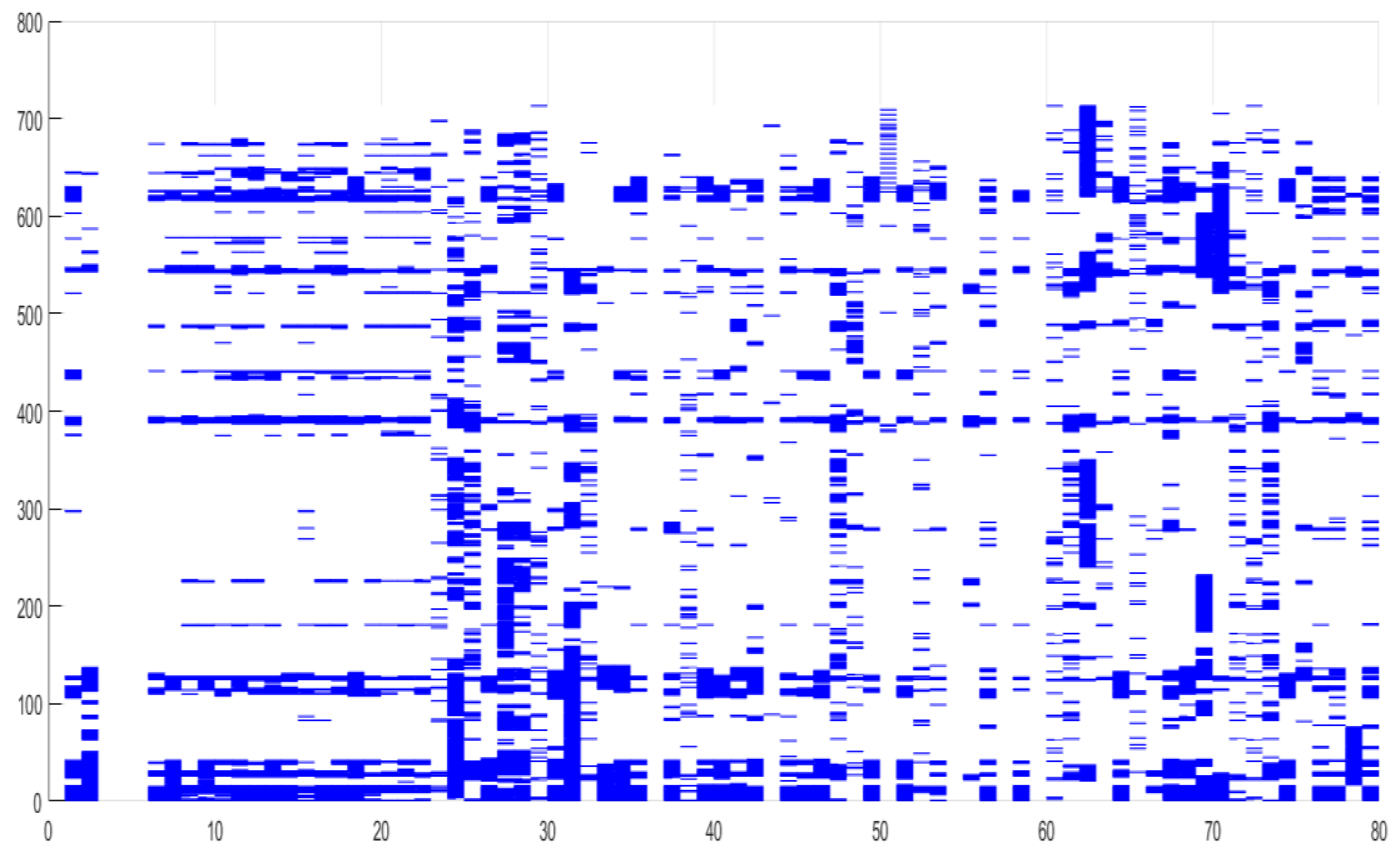
- All the 17 pension funds spend much more time in a low volatility regime in comparison with the open-end investment funds;
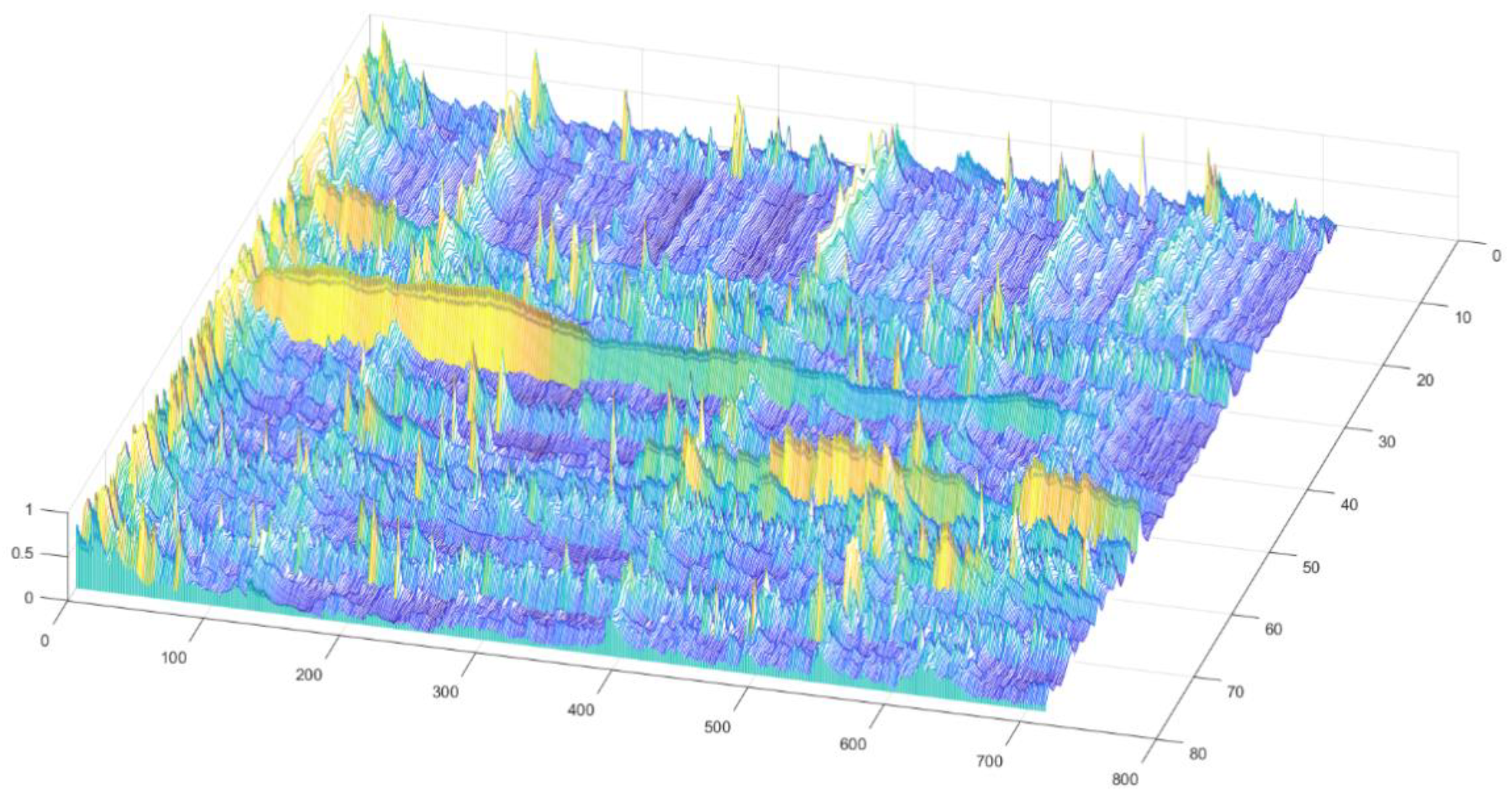
- We can obviously notice at least four distinct periods (around the 120 days mark, respectively the 380, 550 and 600 days marks) when the volatility is rising in synchronization across the entire sample of risk factors and investment vehicles, validating the findings from our Markov Regime Switching model presented earlier.
5. Concluding Remarks
Author Contributions
Funding
Conflicts of Interest
Appendix A

| ADF Decision (1 = Reject H0) | ADF Stat. | ADF p-val | PP Decision (1 = Reject H0) | PP Stat. | PP p-val |
|---|---|---|---|---|---|
| 1 | −14.46251141 | 0.001 | 1 | −25.67207249 | 0.001 |
| 1 | −14.71749747 | 0.001 | 1 | −25.51670332 | 0.001 |
| 1 | −13.74619771 | 0.001 | 1 | −19.85175769 77 | 0.001 |
| 1 | −14.4168156868 | 0.001 | 1 | −26.8227921222212 | 0.001 |
| 1 | −15.67140624 | 0.001 | 1 | −29.93817398 | 0.001 |
| 1 | −13.75150867 | 0.001 | 1 | −23.04230664 | 0.001 |
| 1 | −14.41510806 | 0.001 | 1 | −24.44678857 | 0.001 |
| 1 | −14.4866469 | 0.001 | 1 | −23.38573455 | 0.001 |
| 1 | −14.47350004 | 0.001 | 1 | −23.99653015 | 0.001 |
| 1 | −14.04165656 | 0.001 | 1 | −22.87545243 | 0.001 |
| 1 | −14.4701186 | 0.001 | 1 | −23.01454428 | 0.001 |
| 1 | −14.1895212 | 0.001 | 1 | −22.86211801 | 0.001 |
| 1 | −14.27777585 | 0.001 | 1 | −24.14545206 | 0.001 |
| 1 | −13.80303273 | 0.001 | 1 | −23.35305106 | 0.001 |
| 1 | −13.39487642 | 0.001 | 1 | −21.92481766 | 0.001 |
| 1 | −14.21605846 | 0.001 | 1 | −23.69233346 | 0.001 |
| 1 | −14.37602787 | 0.001 | 1 | −23.5253996 | 0.001 |
| 1 | −13.66510147 | 0.001 | 1 | −23.76110164 | 0.001 |
| 1 | −13.87090243 | 0.001 | 1 | −23.72548999 | 0.001 |
| 1 | −13.74141757 | 0.001 | 1 | −23.90521158 | 0.001 |
| 1 | −14.24952924 | 0.001 | 1 | −23.8385252 | 0.001 |
| 1 | −14.24785231 | 0.001 | 1 | −23.74825187 | 0.001 |
| 1 | −18.1211981 | 0.001 | 1 | −29.3784282 | 0.001 |
| 1 | −14.97054851 | 0.001 | 1 | −24.91489984 | 0.001 |
| 1 | −16.89458682 | 0.001 | 1 | −27.61849966 | 0.001 |
| 1 | −14.52044268 | 0.001 | 1 | −24.93244131 | 0.001 |
| 1 | −12.46749362 | 0.001 | 1 | −20.26554129 | 0.001 |
| 1 | −13.10381388 | 0.001 | 1 | −20.15919968 | 0.001 |
| 1 | −16.3976785 | 0.001 | 1 | −26.97416838 | 0.001 |
| 1 | −14.50648437 | 0.001 | 1 | −24.93350715 | 0.001 |
| 1 | −15.9390632 | 0.001 | 1 | −25.98586152 | 0.001 |
| 1 | −15.69851605 | 0.001 | 1 | −27.27256422 | 0.001 |
| 1 | −16.10313129 | 0.001 | 1 | −26.30189119 | 0.001 |
| 1 | −14.9679989 | 0.001 | 1 | −25.3594308 | 0.001 |
| 1 | −14.03266587 | 0.001 | 1 | −24.25485892 | 0.001 |
| 1 | −16.91314654 | 0.001 | 1 | −26.45163322 | 0.001 |
| 1 | −14.21550375 | 0.001 | 1 | −25.76631002 | 0.001 |
| 1 | −14.92956849 | 0.001 | 1 | −26.99957675 | 0.001 |
| 1 | −13.05578484 | 0.001 | 1 | −23.43650104 | 0.001 |
| 1 | −14.49539819 | 0.001 | 1 | −25.15423069 | 0.001 |
| 1 | −12.8688277 | 0.001 | 1 | −25.70748782 | 0.001 |
| 1 | −14.04295952 | 0.001 | 1 | −25.65288941 | 0.001 |
| 1 | −18.55848773 | 0.001 | 1 | −34.48171394 | 0.001 |
| 1 | −13.60773064 | 0.001 | 1 | −24.8948011 | 0.001 |
| 1 | −14.32807956 | 0.001 | 1 | −25.62962947 | 0.001 |
| 1 | −13.95732154 | 0.001 | 1 | −23.91387015 | 0.001 |
| 1 | −16.51992869 | 0.001 | 1 | −26.70605947 | 0.001 |
| 1 | −12.78280984 | 0.001 | 1 | −20.72170805 | 0.001 |
| 1 | −13.87657218 | 0.001 | 1 | −24.61641683 | 0.001 |
| 1 | −24.22159923 | 0.001 | 1 | −36.97449018 | 0.001 |
| 1 | −14.36223355 | 0.001 | 1 | −25.12178851 | 0.001 |
| 1 | −16.26959953 | 0.001 | 1 | −26.82410925 | 0.001 |
| 1 | −14.20075727 | 0.001 | 1 | −24.91899659 | 0.001 |
| 1 | −15.35569887 | 0.001 | 1 | −26.60584895 | 0.001 |
| 1 | −16.82736412 | 0.001 | 1 | −25.89463779 | 0.001 |
| 1 | −13.48370875 | 0.001 | 1 | −23.38590829 | 0.001 |
| 1 | −14.20732995 | 0.001 | 1 | −22.68135885 | 0.001 |
| 1 | −13.65983931 | 0.001 | 1 | −24.76354594 | 0.001 |
| 1 | −14.56761485 | 0.001 | 1 | −26.15871607 | 0.001 |
| 1 | −16.62121155 | 0.001 | 1 | −27.19126885 | 0.001 |
| 1 | −16.6115905 | 0.001 | 1 | −27.96499086 | 0.001 |
| 1 | −13.11616317 | 0.001 | 1 | −26.09995507 | 0.001 |
| 1 | −14.34763599 | 0.001 | 1 | −23.32187934 | 0.001 |
| 1 | −14.03373819 | 0.001 | 1 | −25.18013417 | 0.001 |
| 1 | −13.04567299 | 0.001 | 1 | −24.13211352 | 0.001 |
| 1 | −14.05197831 | 0.001 | 1 | −24.1261206 | 0.001 |
| 1 | −14.29504014 | 0.001 | 1 | −23.90422506 | 0.001 |
| 1 | −14.09690135 | 0.001 | 1 | −22.79890201 | 0.001 |
| 1 | −14.96805238 | 0.001 | 1 | −27.16497495 | 0.001 |
| 1 | −12.79617163 | 0.001 | 1 | −22.67497103 | 0.001 |
| 1 | −15.56014394 | 0.001 | 1 | −28.49937953 | 0.001 |
| 1 | −16.66734214 | 0.001 | 1 | −27.21580369 | 0.001 |
| 1 | −16.45011689 | 0.001 | 1 | −27.96922127 | 0.001 |
| 1 | −13.9101931 | 0.001 | 1 | −25.00185685 | 0.001 |
| 1 | −11.39738538 | 0.001 | 1 | −16.91914925 | 0.001 |
| 1 | −13.75150917 | 0.001 | 1 | −24.35755956 | 0.001 |
| 1 | −13.73742592 | 0.001 | 1 | −24.30617894 | 0.001 |
| 1 | −15.35690246 | 0.001 | 1 | −23.02156195 | 0.001 |
| 1 | −13.48500411 | 0.001 | 1 | −22.9360866 | 0.001 |
| 1 | −14.61724683 | 0.001 | 1 | −22.941735 | 0.001 |
| 1 | −13.4318641 | 0.001 | 1 | −19.76030578 | 0.001 |
| 1 | −14.66877486 | 0.001 | 1 | −24.54519058 | 0.001 |
| 1 | −13.54439039 | 0.001 | 1 | −19.98432505 | 0.001 |
| 1 | −15.39654954 | 0.001 | 1 | −26.97519709 | 0.001 |
| 1 | −12.94530177 | 0.001 | 1 | −20.15765856 | 0.001 |
| BET Volatility Regimes | STOXX Volatility Regimes | BONDS/RON Volatility Regimes | BONDS/EUR Volatility Regimes | EUR/RON Volatility Regimes | ||||||||||||||||
|---|---|---|---|---|---|---|---|---|---|---|---|---|---|---|---|---|---|---|---|---|
| LOW | HIGH | LOW | HIGH | LOW | HIGH | LOW | HIGH | LOW | HIGH | |||||||||||
| mean | std | mean | std | mean | std | mean | std | mean | std | mean | std | mean | std | mean | std | mean | std | mean | std | |
| v01 | 0.0014 | 0.0002 | 0.0018 | 0.0004 | 0.0014 | 0.0002 | 0.0018 | 0.0004 | 0.0014 | 0.0003 | 0.0015 | 0.0004 | 0.0014 | 0.0003 | 0.0014 | 0.0003 | 0.0014 | 0.0003 | 0.0014 | 0.0003 |
| v02 | 0.0016 | 0.0003 | 0.0023 | 0.0007 | 0.0016 | 0.0003 | 0.0024 | 0.0006 | 0.0017 | 0.0004 | 0.0018 | 0.0006 | 0.0017 | 0.0005 | 0.0017 | 0.0004 | 0.0017 | 0.0005 | 0.0017 | 0.0004 |
| v03 | 0.0015 | 0.0003 | 0.0022 | 0.0008 | 0.0016 | 0.0004 | 0.0020 | 0.0007 | 0.0016 | 0.0004 | 0.0018 | 0.0007 | 0.0016 | 0.0004 | 0.0016 | 0.0005 | 0.0016 | 0.0004 | 0.0016 | 0.0006 |
| v04 | 0.0013 | 0.0003 | 0.0020 | 0.0006 | 0.0013 | 0.0003 | 0.0020 | 0.0006 | 0.0014 | 0.0004 | 0.0016 | 0.0006 | 0.0014 | 0.0004 | 0.0014 | 0.0004 | 0.0014 | 0.0004 | 0.0014 | 0.0005 |
| v05 | 0.0015 | 0.0003 | 0.0022 | 0.0006 | 0.0015 | 0.0003 | 0.0021 | 0.0006 | 0.0016 | 0.0004 | 0.0017 | 0.0005 | 0.0016 | 0.0004 | 0.0016 | 0.0004 | 0.0016 | 0.0004 | 0.0016 | 0.0004 |
| v06 | 0.0014 | 0.0003 | 0.0020 | 0.0006 | 0.0014 | 0.0003 | 0.0020 | 0.0006 | 0.0014 | 0.0003 | 0.0017 | 0.0005 | 0.0015 | 0.0004 | 0.0015 | 0.0004 | 0.0015 | 0.0004 | 0.0015 | 0.0004 |
| v07 | 0.0016 | 0.0003 | 0.0023 | 0.0007 | 0.0016 | 0.0004 | 0.0022 | 0.0007 | 0.0016 | 0.0004 | 0.0019 | 0.0006 | 0.0017 | 0.0005 | 0.0016 | 0.0005 | 0.0017 | 0.0005 | 0.0017 | 0.0005 |
| v08 | 0.0020 | 0.0004 | 0.0030 | 0.0009 | 0.0020 | 0.0004 | 0.0030 | 0.0009 | 0.0021 | 0.0005 | 0.0023 | 0.0008 | 0.0022 | 0.0006 | 0.0021 | 0.0006 | 0.0022 | 0.0006 | 0.0021 | 0.0006 |
| v09 | 0.0015 | 0.0002 | 0.0021 | 0.0005 | 0.0015 | 0.0003 | 0.0020 | 0.0005 | 0.0016 | 0.0003 | 0.0017 | 0.0004 | 0.0016 | 0.0004 | 0.0016 | 0.0003 | 0.0016 | 0.0004 | 0.0016 | 0.0004 |
| v10 | 0.0014 | 0.0003 | 0.0020 | 0.0006 | 0.0014 | 0.0003 | 0.0019 | 0.0006 | 0.0014 | 0.0004 | 0.0016 | 0.0005 | 0.0015 | 0.0004 | 0.0014 | 0.0004 | 0.0015 | 0.0004 | 0.0014 | 0.0004 |
| v11 | 0.0016 | 0.0003 | 0.0023 | 0.0008 | 0.0016 | 0.0004 | 0.0021 | 0.0007 | 0.0016 | 0.0004 | 0.0018 | 0.0007 | 0.0017 | 0.0005 | 0.0017 | 0.0005 | 0.0017 | 0.0004 | 0.0017 | 0.0006 |
| v12 | 0.0015 | 0.0003 | 0.0020 | 0.0006 | 0.0015 | 0.0003 | 0.0020 | 0.0006 | 0.0015 | 0.0003 | 0.0017 | 0.0005 | 0.0016 | 0.0004 | 0.0015 | 0.0004 | 0.0015 | 0.0004 | 0.0015 | 0.0004 |
| v13 | 0.0020 | 0.0004 | 0.0030 | 0.0008 | 0.0020 | 0.0004 | 0.0030 | 0.0008 | 0.0021 | 0.0005 | 0.0023 | 0.0007 | 0.0021 | 0.0006 | 0.0022 | 0.0006 | 0.0021 | 0.0006 | 0.0022 | 0.0006 |
| v14 | 0.0015 | 0.0003 | 0.0021 | 0.0005 | 0.0015 | 0.0002 | 0.0021 | 0.0006 | 0.0016 | 0.0003 | 0.0018 | 0.0005 | 0.0016 | 0.0004 | 0.0016 | 0.0004 | 0.0016 | 0.0004 | 0.0016 | 0.0004 |
| v15 | 0.0017 | 0.0003 | 0.0023 | 0.0005 | 0.0017 | 0.0003 | 0.0022 | 0.0006 | 0.0018 | 0.0004 | 0.0019 | 0.0004 | 0.0018 | 0.0004 | 0.0018 | 0.0004 | 0.0018 | 0.0004 | 0.0018 | 0.0004 |
| v16 | 0.0014 | 0.0003 | 0.0020 | 0.0006 | 0.0014 | 0.0003 | 0.0020 | 0.0006 | 0.0015 | 0.0004 | 0.0016 | 0.0005 | 0.0015 | 0.0004 | 0.0015 | 0.0004 | 0.0015 | 0.0004 | 0.0015 | 0.0004 |
| v17 | 0.0017 | 0.0003 | 0.0023 | 0.0006 | 0.0017 | 0.0003 | 0.0022 | 0.0006 | 0.0017 | 0.0004 | 0.0019 | 0.0005 | 0.0018 | 0.0004 | 0.0017 | 0.0004 | 0.0018 | 0.0004 | 0.0017 | 0.0004 |
| v18 | 0.0193 | 0.0034 | 0.0179 | 0.0037 | 0.0193 | 0.0034 | 0.0185 | 0.0037 | 0.0191 | 0.0033 | 0.0195 | 0.0041 | 0.0191 | 0.0032 | 0.0192 | 0.0038 | 0.0191 | 0.0035 | 0.0192 | 0.0034 |
| v19 | 0.0065 | 0.0024 | 0.0087 | 0.0032 | 0.0061 | 0.0020 | 0.0107 | 0.0027 | 0.0068 | 0.0026 | 0.0069 | 0.0027 | 0.0067 | 0.0028 | 0.0069 | 0.0025 | 0.0068 | 0.0027 | 0.0066 | 0.0026 |
| v20 | 0.0015 | 0.0003 | 0.0015 | 0.0003 | 0.0015 | 0.0003 | 0.0015 | 0.0003 | 0.0015 | 0.0003 | 0.0015 | 0.0003 | 0.0014 | 0.0003 | 0.0015 | 0.0002 | 0.0014 | 0.0002 | 0.0016 | 0.0003 |
| v21 | 0.0049 | 0.0012 | 0.0075 | 0.0028 | 0.0047 | 0.0009 | 0.0082 | 0.0026 | 0.0051 | 0.0015 | 0.0058 | 0.0024 | 0.0052 | 0.0018 | 0.0053 | 0.0017 | 0.0053 | 0.0018 | 0.0052 | 0.0017 |
| v22 | 0.0006 | 0.0003 | 0.0007 | 0.0004 | 0.0006 | 0.0003 | 0.0008 | 0.0004 | 0.0006 | 0.0003 | 0.0008 | 0.0004 | 0.0005 | 0.0003 | 0.0007 | 0.0003 | 0.0006 | 0.0003 | 0.0007 | 0.0003 |
| v23 | 0.0004 | 0.0001 | 0.0005 | 0.0002 | 0.0004 | 0.0001 | 0.0005 | 0.0002 | 0.0004 | 0.0001 | 0.0005 | 0.0002 | 0.0004 | 0.0002 | 0.0004 | 0.0001 | 0.0004 | 0.0002 | 0.0004 | 0.0001 |
| v24 | 0.0048 | 0.0005 | 0.0049 | 0.0007 | 0.0048 | 0.0005 | 0.0048 | 0.0006 | 0.0048 | 0.0005 | 0.0048 | 0.0005 | 0.0048 | 0.0005 | 0.0049 | 0.0005 | 0.0048 | 0.0005 | 0.0049 | 0.0006 |
| v25 | 0.0011 | 0.0002 | 0.0016 | 0.0005 | 0.0011 | 0.0002 | 0.0017 | 0.0005 | 0.0011 | 0.0003 | 0.0012 | 0.0005 | 0.0011 | 0.0004 | 0.0012 | 0.0003 | 0.0011 | 0.0004 | 0.0012 | 0.0003 |
| v26 | 0.0019 | 0.0006 | 0.0024 | 0.0010 | 0.0018 | 0.0006 | 0.0029 | 0.0008 | 0.0019 | 0.0007 | 0.0021 | 0.0008 | 0.0018 | 0.0006 | 0.0021 | 0.0007 | 0.0019 | 0.0007 | 0.0022 | 0.0007 |
| v27 | 0.0015 | 0.0003 | 0.0016 | 0.0003 | 0.0015 | 0.0003 | 0.0016 | 0.0003 | 0.0015 | 0.0003 | 0.0016 | 0.0003 | 0.0015 | 0.0003 | 0.0016 | 0.0003 | 0.0015 | 0.0003 | 0.0017 | 0.0004 |
| v28 | 0.0081 | 0.0021 | 0.0119 | 0.0047 | 0.0078 | 0.0014 | 0.0135 | 0.0042 | 0.0084 | 0.0025 | 0.0096 | 0.0042 | 0.0086 | 0.0027 | 0.0087 | 0.0031 | 0.0086 | 0.0029 | 0.0087 | 0.0029 |
| v29 | 0.0060 | 0.0014 | 0.0092 | 0.0034 | 0.0058 | 0.0010 | 0.0099 | 0.0032 | 0.0063 | 0.0019 | 0.0070 | 0.0028 | 0.0064 | 0.0022 | 0.0065 | 0.0021 | 0.0065 | 0.0022 | 0.0064 | 0.0020 |
| v30 | 0.0049 | 0.0010 | 0.0073 | 0.0025 | 0.0049 | 0.0009 | 0.0074 | 0.0026 | 0.0052 | 0.0014 | 0.0057 | 0.0019 | 0.0054 | 0.0017 | 0.0051 | 0.0014 | 0.0053 | 0.0016 | 0.0052 | 0.0013 |
| v31 | 0.0002 | 0.0001 | 0.0002 | 0.0001 | 0.0002 | 0.0001 | 0.0002 | 0.0000 | 0.0002 | 0.0001 | 0.0002 | 0.0001 | 0.0002 | 0.0001 | 0.0002 | 0.0001 | 0.0002 | 0.0001 | 0.0002 | 0.0001 |
| v32 | 0.0023 | 0.0005 | 0.0035 | 0.0012 | 0.0023 | 0.0004 | 0.0037 | 0.0011 | 0.0025 | 0.0007 | 0.0027 | 0.0009 | 0.0025 | 0.0008 | 0.0025 | 0.0007 | 0.0025 | 0.0007 | 0.0026 | 0.0007 |
| v33 | 0.0002 | 0.0001 | 0.0002 | 0.0001 | 0.0002 | 0.0001 | 0.0002 | 0.0001 | 0.0002 | 0.0001 | 0.0002 | 0.0001 | 0.0002 | 0.0001 | 0.0002 | 0.0001 | 0.0002 | 0.0001 | 0.0002 | 0.0001 |
| v34 | 0.0039 | 0.0009 | 0.0060 | 0.0021 | 0.0038 | 0.0007 | 0.0063 | 0.0021 | 0.0041 | 0.0013 | 0.0045 | 0.0018 | 0.0042 | 0.0015 | 0.0042 | 0.0012 | 0.0042 | 0.0014 | 0.0042 | 0.0013 |
| v35 | 0.0062 | 0.0013 | 0.0096 | 0.0030 | 0.0062 | 0.0012 | 0.0095 | 0.0031 | 0.0066 | 0.0018 | 0.0072 | 0.0026 | 0.0067 | 0.0021 | 0.0067 | 0.0019 | 0.0067 | 0.0021 | 0.0067 | 0.0018 |
| v36 | 0.0060 | 0.0015 | 0.0088 | 0.0034 | 0.0058 | 0.0010 | 0.0097 | 0.0032 | 0.0063 | 0.0019 | 0.0068 | 0.0026 | 0.0065 | 0.0023 | 0.0062 | 0.0018 | 0.0064 | 0.0021 | 0.0063 | 0.0019 |
| v37 | 0.0036 | 0.0010 | 0.0056 | 0.0025 | 0.0035 | 0.0010 | 0.0056 | 0.0024 | 0.0038 | 0.0013 | 0.0041 | 0.0020 | 0.0039 | 0.0017 | 0.0038 | 0.0013 | 0.0039 | 0.0015 | 0.0038 | 0.0013 |
| v38 | 0.0018 | 0.0217 | 0.0002 | 0.0001 | 0.0018 | 0.0218 | 0.0002 | 0.0001 | 0.0013 | 0.0173 | 0.0026 | 0.0287 | 0.0012 | 0.0175 | 0.0020 | 0.0228 | 0.0018 | 0.0222 | 0.0002 | 0.0001 |
| v39 | 0.0019 | 0.0004 | 0.0027 | 0.0008 | 0.0019 | 0.0003 | 0.0029 | 0.0008 | 0.0020 | 0.0005 | 0.0021 | 0.0007 | 0.0021 | 0.0006 | 0.0020 | 0.0005 | 0.0020 | 0.0006 | 0.0020 | 0.0005 |
| v40 | 0.0059 | 0.0015 | 0.0098 | 0.0045 | 0.0058 | 0.0011 | 0.0101 | 0.0045 | 0.0063 | 0.0023 | 0.0071 | 0.0033 | 0.0066 | 0.0029 | 0.0063 | 0.0020 | 0.0065 | 0.0026 | 0.0064 | 0.0021 |
| v41 | 0.0030 | 0.0007 | 0.0047 | 0.0016 | 0.0029 | 0.0006 | 0.0048 | 0.0016 | 0.0032 | 0.0010 | 0.0035 | 0.0013 | 0.0033 | 0.0011 | 0.0032 | 0.0010 | 0.0032 | 0.0011 | 0.0032 | 0.0009 |
| v42 | 0.0015 | 0.0003 | 0.0016 | 0.0003 | 0.0015 | 0.0003 | 0.0015 | 0.0002 | 0.0015 | 0.0003 | 0.0015 | 0.0003 | 0.0015 | 0.0003 | 0.0016 | 0.0002 | 0.0015 | 0.0003 | 0.0016 | 0.0003 |
| v43 | 0.0005 | 0.0001 | 0.0005 | 0.0002 | 0.0005 | 0.0001 | 0.0005 | 0.0001 | 0.0005 | 0.0001 | 0.0006 | 0.0002 | 0.0005 | 0.0001 | 0.0005 | 0.0001 | 0.0005 | 0.0001 | 0.0005 | 0.0002 |
| v44 | 0.0049 | 0.0010 | 0.0075 | 0.0026 | 0.0048 | 0.0010 | 0.0075 | 0.0025 | 0.0051 | 0.0015 | 0.0056 | 0.0020 | 0.0054 | 0.0018 | 0.0051 | 0.0015 | 0.0053 | 0.0017 | 0.0051 | 0.0015 |
| v45 | 0.0008 | 0.0016 | 0.0007 | 0.0011 | 0.0009 | 0.0016 | 0.0003 | 0.0003 | 0.0008 | 0.0016 | 0.0007 | 0.0010 | 0.0008 | 0.0008 | 0.0007 | 0.0020 | 0.0008 | 0.0016 | 0.0007 | 0.0011 |
| v46 | 0.0065 | 0.0013 | 0.0099 | 0.0031 | 0.0064 | 0.0013 | 0.0098 | 0.0031 | 0.0068 | 0.0019 | 0.0075 | 0.0026 | 0.0070 | 0.0022 | 0.0069 | 0.0019 | 0.0070 | 0.0021 | 0.0069 | 0.0019 |
| v47 | 0.0013 | 0.0003 | 0.0014 | 0.0003 | 0.0013 | 0.0003 | 0.0014 | 0.0003 | 0.0013 | 0.0003 | 0.0013 | 0.0003 | 0.0013 | 0.0004 | 0.0013 | 0.0003 | 0.0013 | 0.0004 | 0.0013 | 0.0002 |
| v48 | 0.0036 | 0.0008 | 0.0052 | 0.0017 | 0.0036 | 0.0008 | 0.0052 | 0.0016 | 0.0038 | 0.0010 | 0.0041 | 0.0015 | 0.0039 | 0.0011 | 0.0038 | 0.0011 | 0.0039 | 0.0012 | 0.0038 | 0.0009 |
| v49 | 0.0011 | 0.0005 | 0.0008 | 0.0005 | 0.0011 | 0.0005 | 0.0005 | 0.0004 | 0.0010 | 0.0005 | 0.0010 | 0.0006 | 0.0012 | 0.0005 | 0.0009 | 0.0005 | 0.0010 | 0.0005 | 0.0010 | 0.0005 |
| v50 | 0.0018 | 0.0003 | 0.0019 | 0.0004 | 0.0019 | 0.0003 | 0.0019 | 0.0003 | 0.0018 | 0.0003 | 0.0020 | 0.0004 | 0.0018 | 0.0003 | 0.0019 | 0.0003 | 0.0018 | 0.0003 | 0.0020 | 0.0004 |
| v51 | 0.0047 | 0.0010 | 0.0070 | 0.0026 | 0.0046 | 0.0009 | 0.0070 | 0.0025 | 0.0049 | 0.0014 | 0.0053 | 0.0019 | 0.0051 | 0.0017 | 0.0049 | 0.0013 | 0.0050 | 0.0016 | 0.0049 | 0.0014 |
| v52 | 0.0029 | 0.0010 | 0.0028 | 0.0017 | 0.0030 | 0.0010 | 0.0020 | 0.0014 | 0.0028 | 0.0010 | 0.0030 | 0.0012 | 0.0029 | 0.0011 | 0.0027 | 0.0010 | 0.0028 | 0.0010 | 0.0030 | 0.0013 |
| v53 | 0.0046 | 0.0009 | 0.0070 | 0.0024 | 0.0046 | 0.0009 | 0.0069 | 0.0023 | 0.0048 | 0.0014 | 0.0053 | 0.0019 | 0.0050 | 0.0016 | 0.0048 | 0.0013 | 0.0049 | 0.0015 | 0.0048 | 0.0013 |
| v54 | 0.0001 | 0.0002 | 0.0001 | 0.0001 | 0.0001 | 0.0002 | 0.0001 | 0.0001 | 0.0001 | 0.0002 | 0.0001 | 0.0001 | 0.0001 | 0.0003 | 0.0001 | 0.0000 | 0.0001 | 0.0002 | 0.0001 | 0.0000 |
| v55 | 0.0050 | 0.0005 | 0.0051 | 0.0007 | 0.0050 | 0.0005 | 0.0051 | 0.0007 | 0.0051 | 0.0005 | 0.0051 | 0.0006 | 0.0050 | 0.0006 | 0.0051 | 0.0006 | 0.0050 | 0.0005 | 0.0051 | 0.0007 |
| v56 | 0.0014 | 0.0003 | 0.0015 | 0.0003 | 0.0014 | 0.0003 | 0.0015 | 0.0003 | 0.0014 | 0.0003 | 0.0015 | 0.0003 | 0.0014 | 0.0003 | 0.0015 | 0.0002 | 0.0014 | 0.0002 | 0.0016 | 0.0003 |
| v57 | 0.0023 | 0.0008 | 0.0027 | 0.0013 | 0.0024 | 0.0008 | 0.0026 | 0.0013 | 0.0024 | 0.0009 | 0.0025 | 0.0009 | 0.0024 | 0.0010 | 0.0024 | 0.0007 | 0.0024 | 0.0009 | 0.0024 | 0.0009 |
| v58 | 0.0021 | 0.0003 | 0.0022 | 0.0006 | 0.0021 | 0.0004 | 0.0021 | 0.0005 | 0.0021 | 0.0004 | 0.0021 | 0.0004 | 0.0022 | 0.0004 | 0.0021 | 0.0003 | 0.0021 | 0.0004 | 0.0021 | 0.0004 |
| v59 | 0.0029 | 0.0005 | 0.0041 | 0.0012 | 0.0028 | 0.0004 | 0.0042 | 0.0012 | 0.0030 | 0.0007 | 0.0032 | 0.0010 | 0.0031 | 0.0009 | 0.0030 | 0.0007 | 0.0030 | 0.0008 | 0.0030 | 0.0007 |
| v60 | 0.0002 | 0.0001 | 0.0002 | 0.0002 | 0.0002 | 0.0001 | 0.0002 | 0.0001 | 0.0002 | 0.0001 | 0.0002 | 0.0001 | 0.0002 | 0.0001 | 0.0002 | 0.0001 | 0.0002 | 0.0001 | 0.0002 | 0.0001 |
| v61 | 0.0042 | 0.0009 | 0.0058 | 0.0018 | 0.0042 | 0.0007 | 0.0061 | 0.0017 | 0.0044 | 0.0011 | 0.0047 | 0.0014 | 0.0045 | 0.0012 | 0.0044 | 0.0011 | 0.0045 | 0.0012 | 0.0044 | 0.0011 |
| v62 | 0.0030 | 0.0005 | 0.0041 | 0.0009 | 0.0030 | 0.0005 | 0.0040 | 0.0009 | 0.0031 | 0.0007 | 0.0033 | 0.0008 | 0.0032 | 0.0006 | 0.0031 | 0.0008 | 0.0031 | 0.0007 | 0.0031 | 0.0007 |
| v63 | 0.0035 | 0.0007 | 0.0051 | 0.0017 | 0.0034 | 0.0006 | 0.0054 | 0.0015 | 0.0037 | 0.0010 | 0.0039 | 0.0013 | 0.0038 | 0.0012 | 0.0036 | 0.0009 | 0.0037 | 0.0011 | 0.0036 | 0.0009 |
| v64 | 0.0023 | 0.0010 | 0.0028 | 0.0013 | 0.0022 | 0.0009 | 0.0033 | 0.0015 | 0.0023 | 0.0011 | 0.0024 | 0.0010 | 0.0023 | 0.0012 | 0.0024 | 0.0010 | 0.0024 | 0.0011 | 0.0023 | 0.0010 |
| v65 | 0.0010 | 0.0005 | 0.0014 | 0.0006 | 0.0009 | 0.0004 | 0.0014 | 0.0007 | 0.0010 | 0.0005 | 0.0011 | 0.0004 | 0.0012 | 0.0006 | 0.0009 | 0.0003 | 0.0010 | 0.0005 | 0.0009 | 0.0004 |
| v66 | 0.0016 | 0.0003 | 0.0018 | 0.0004 | 0.0016 | 0.0003 | 0.0018 | 0.0004 | 0.0016 | 0.0003 | 0.0017 | 0.0003 | 0.0016 | 0.0003 | 0.0016 | 0.0003 | 0.0016 | 0.0003 | 0.0017 | 0.0004 |
| v67 | 0.0050 | 0.0005 | 0.0051 | 0.0008 | 0.0050 | 0.0006 | 0.0051 | 0.0007 | 0.0050 | 0.0006 | 0.0051 | 0.0006 | 0.0050 | 0.0006 | 0.0051 | 0.0006 | 0.0050 | 0.0005 | 0.0051 | 0.0007 |
| v68 | 0.0014 | 0.0003 | 0.0015 | 0.0003 | 0.0014 | 0.0003 | 0.0015 | 0.0002 | 0.0014 | 0.0003 | 0.0015 | 0.0003 | 0.0014 | 0.0003 | 0.0015 | 0.0002 | 0.0014 | 0.0002 | 0.0016 | 0.0003 |
| v69 | 0.0048 | 0.0010 | 0.0074 | 0.0026 | 0.0048 | 0.0009 | 0.0077 | 0.0024 | 0.0051 | 0.0015 | 0.0056 | 0.0021 | 0.0053 | 0.0018 | 0.0051 | 0.0015 | 0.0052 | 0.0017 | 0.0052 | 0.0015 |
| v70 | 0.0001 | 0.0001 | 0.0001 | 0.0000 | 0.0001 | 0.0001 | 0.0001 | 0.0000 | 0.0001 | 0.0000 | 0.0002 | 0.0001 | 0.0001 | 0.0001 | 0.0001 | 0.0000 | 0.0001 | 0.0001 | 0.0002 | 0.0001 |
| v71 | 0.0018 | 0.0004 | 0.0027 | 0.0008 | 0.0018 | 0.0003 | 0.0027 | 0.0008 | 0.0019 | 0.0005 | 0.0020 | 0.0007 | 0.0020 | 0.0006 | 0.0019 | 0.0005 | 0.0019 | 0.0006 | 0.0019 | 0.0005 |
| v72 | 0.0035 | 0.0007 | 0.0052 | 0.0017 | 0.0034 | 0.0006 | 0.0054 | 0.0017 | 0.0037 | 0.0010 | 0.0039 | 0.0014 | 0.0038 | 0.0012 | 0.0036 | 0.0010 | 0.0037 | 0.0011 | 0.0037 | 0.0010 |
| v73 | 0.0096 | 0.0058 | 0.0136 | 0.0076 | 0.0092 | 0.0045 | 0.0155 | 0.0102 | 0.0102 | 0.0063 | 0.0100 | 0.0059 | 0.0107 | 0.0053 | 0.0095 | 0.0071 | 0.0103 | 0.0063 | 0.0095 | 0.0057 |
| v74 | 0.0036 | 0.0007 | 0.0055 | 0.0018 | 0.0036 | 0.0007 | 0.0056 | 0.0018 | 0.0038 | 0.0011 | 0.0041 | 0.0015 | 0.0039 | 0.0013 | 0.0038 | 0.0010 | 0.0039 | 0.0012 | 0.0038 | 0.0011 |
| v75 | 0.0023 | 0.0004 | 0.0027 | 0.0010 | 0.0022 | 0.0004 | 0.0028 | 0.0009 | 0.0023 | 0.0005 | 0.0025 | 0.0007 | 0.0023 | 0.0006 | 0.0023 | 0.0006 | 0.0023 | 0.0006 | 0.0024 | 0.0007 |
| v76 | 0.0016 | 0.0005 | 0.0022 | 0.0009 | 0.0016 | 0.0004 | 0.0023 | 0.0008 | 0.0017 | 0.0005 | 0.0019 | 0.0006 | 0.0018 | 0.0006 | 0.0017 | 0.0005 | 0.0017 | 0.0006 | 0.0017 | 0.0005 |
| v77 | 0.0019 | 0.0004 | 0.0021 | 0.0007 | 0.0019 | 0.0004 | 0.0022 | 0.0006 | 0.0019 | 0.0004 | 0.0021 | 0.0005 | 0.0019 | 0.0004 | 0.0019 | 0.0004 | 0.0019 | 0.0004 | 0.0020 | 0.0005 |
| v78 | 0.0012 | 0.0004 | 0.0016 | 0.0006 | 0.0012 | 0.0003 | 0.0017 | 0.0006 | 0.0013 | 0.0004 | 0.0014 | 0.0005 | 0.0013 | 0.0005 | 0.0013 | 0.0004 | 0.0013 | 0.0004 | 0.0013 | 0.0004 |
| v79 | 0.0017 | 0.0003 | 0.0018 | 0.0004 | 0.0016 | 0.0003 | 0.0018 | 0.0004 | 0.0016 | 0.0003 | 0.0018 | 0.0004 | 0.0016 | 0.0003 | 0.0017 | 0.0003 | 0.0016 | 0.0003 | 0.0018 | 0.0004 |
| v80 | 0.0008 | 0.0003 | 0.0010 | 0.0003 | 0.0008 | 0.0003 | 0.0010 | 0.0004 | 0.0008 | 0.0003 | 0.0010 | 0.0004 | 0.0009 | 0.0003 | 0.0008 | 0.0003 | 0.0009 | 0.0003 | 0.0009 | 0.0003 |
| Bet Volatility Regimes | STOXX Volatility Regimes | BONDS/RON Volatility Regimes | BONDS/EUR Volatility Regimes | EUR/RON Volatility Regimes | ||||||||||||||||
|---|---|---|---|---|---|---|---|---|---|---|---|---|---|---|---|---|---|---|---|---|
| LOW | HIGH | LOW | HIGH | LOW | HIGH | LOW | HIGH | LOW | HIGH | |||||||||||
| mean | std | mean | std | mean | std | mean | std | mean | std | mean | std | mean | std | mean | std | mean | std | mean | std | |
| v01 | 0.7537 | 0.0715 | 0.7808 | 0.1694 | 0.2943 | 0.0267 | 0.3651 | 0.0748 | −0.3506 | 0.0249 | −0.3628 | 0.0432 | 0.0451 | 0.0195 | 0.0420 | 0.0054 | −0.0728 | 0.0105 | −0.0741 | 0.0102 |
| v02 | 0.7184 | 0.0496 | 0.7390 | 0.1089 | 0.6292 | 0.1058 | 0.7970 | 0.0695 | −0.2854 | 0.0372 | −0.3033 | 0.0656 | 0.1167 | 0.0253 | 0.1266 | 0.0607 | −0.0793 | 0.0205 | −0.0816 | 0.0199 |
| v03 | 0.7308 | 0.0649 | 0.7551 | 0.1359 | 0.4690 | 0.0378 | 0.5291 | 0.0917 | −0.3531 | 0.0455 | −0.3687 | 0.0716 | 0.0536 | 0.0159 | 0.0543 | 0.0291 | −0.0256 | 0.0054 | −0.0250 | 0.0004 |
| v04 | 0.7265 | 0.0803 | 0.7564 | 0.1508 | 0.5489 | 0.0713 | 0.6910 | 0.0717 | −0.3555 | 0.0744 | −0.3869 | 0.1048 | 0.0809 | 0.0332 | 0.0889 | 0.0782 | −0.0686 | 0.0108 | −0.0699 | 0.0105 |
| v05 | 0.8478 | 0.0503 | 0.8349 | 0.1642 | 0.2920 | 0.0226 | 0.3863 | 0.0863 | −0.2774 | 0.0563 | −0.2943 | 0.0946 | 0.0455 | 0.0364 | 0.0442 | 0.0281 | −0.0401 | 0.0032 | −0.0397 | 0.0001 |
| v06 | 0.7679 | 0.0702 | 0.7851 | 0.1528 | 0.4672 | 0.0132 | 0.5281 | 0.0629 | −0.3753 | 0.0580 | −0.3994 | 0.0933 | 0.0571 | 0.0233 | 0.0575 | 0.0503 | −0.0302 | 0.0079 | −0.0294 | 0.0022 |
| v07 | 0.7970 | 0.0812 | 0.8031 | 0.1883 | 0.4177 | 0.0296 | 0.5334 | 0.0853 | −0.3504 | 0.0429 | −0.3670 | 0.0684 | 0.0280 | 0.0159 | 0.0259 | 0.0234 | −0.0595 | 0.0145 | −0.0612 | 0.0141 |
| v08 | 0.8369 | 0.0523 | 0.8393 | 0.1547 | 0.4530 | 0.0302 | 0.5243 | 0.0638 | −0.2519 | 0.0591 | −0.2726 | 0.1044 | 0.0678 | 0.0186 | 0.0679 | 0.0407 | −0.0302 | 0.0042 | −0.0297 | 0.0003 |
| v09 | 0.7597 | 0.0632 | 0.7874 | 0.1530 | 0.2871 | 0.0369 | 0.3685 | 0.0801 | −0.3195 | 0.0384 | −0.3346 | 0.0603 | 0.0418 | 0.0117 | 0.0407 | 0.0229 | −0.0531 | 0.0016 | −0.0530 | 0.0000 |
| v10 | 0.8177 | 0.0798 | 0.8020 | 0.2033 | 0.2887 | 0.0359 | 0.4009 | 0.1076 | −0.2425 | 0.0626 | −0.2598 | 0.1009 | 0.0306 | 0.0025 | 0.0304 | 0.0000 | −0.0053 | 0.0083 | −0.0044 | 0.0014 |
| v11 | 0.7436 | 0.0621 | 0.7668 | 0.1422 | 0.4294 | 0.0341 | 0.4971 | 0.0935 | −0.3288 | 0.0471 | −0.3441 | 0.0769 | 0.0681 | 0.0417 | 0.0679 | 0.0328 | −0.0114 | 0.0070 | −0.0106 | 0.0010 |
| v12 | 0.7817 | 0.0687 | 0.7996 | 0.1580 | 0.4573 | 0.0187 | 0.5081 | 0.0530 | −0.3511 | 0.0548 | −0.3759 | 0.0925 | 0.0534 | 0.0184 | 0.0540 | 0.0355 | −0.0248 | 0.0053 | −0.0241 | 0.0006 |
| v13 | 0.7999 | 0.0548 | 0.8096 | 0.1511 | 0.2881 | 0.0435 | 0.3822 | 0.0859 | −0.2292 | 0.0528 | −0.2423 | 0.0870 | 0.0495 | 0.0164 | 0.0483 | 0.0356 | −0.0462 | 0.0015 | −0.0460 | 0.0000 |
| v14 | 0.8353 | 0.0683 | 0.8320 | 0.1863 | 0.3297 | 0.0096 | 0.4040 | 0.0765 | −0.2972 | 0.0545 | −0.3190 | 0.0966 | 0.0449 | 0.0337 | 0.0436 | 0.0260 | −0.0444 | 0.0006 | −0.0443 | 0.0000 |
| v15 | 0.8113 | 0.0703 | 0.8073 | 0.1878 | 0.2838 | 0.0392 | 0.3853 | 0.0833 | −0.3028 | 0.0429 | −0.3215 | 0.0801 | 0.0579 | 0.0215 | 0.0593 | 0.0170 | −0.0468 | 0.0001 | −0.0468 | 0.0000 |
| v16 | 0.7865 | 0.0871 | 0.8060 | 0.1753 | 0.4329 | 0.0474 | 0.5464 | 0.0742 | −0.3519 | 0.0604 | −0.3751 | 0.0895 | 0.0622 | 0.0155 | 0.0627 | 0.0390 | −0.0542 | 0.0008 | −0.0542 | 0.0006 |
| v17 | 0.8162 | 0.1006 | 0.8182 | 0.2149 | 0.3714 | 0.0107 | 0.4375 | 0.0658 | −0.3401 | 0.0396 | −0.3567 | 0.0681 | 0.0622 | 0.0419 | 0.0625 | 0.0329 | −0.0583 | 0.0077 | −0.0592 | 0.0074 |
| v18 | 0.1613 | 0.0498 | 0.2827 | 0.1918 | 0.0873 | 0.0453 | 0.3120 | 0.1991 | −0.0525 | 0.0087 | −0.0542 | 0.0106 | 0.0812 | 0.0383 | 0.0820 | 0.0291 | −0.0569 | 0.0402 | −0.0481 | 0.0635 |
| v19 | 0.2307 | 0.0743 | 0.2870 | 0.1358 | 0.0918 | 0.0910 | 0.3000 | 0.1356 | 0.0156 | 0.1110 | −0.0055 | 0.1529 | 0.0202 | 0.0420 | 0.0263 | 0.0185 | 0.0387 | 0.0416 | 0.0455 | 0.0521 |
| v20 | −0.0431 | 0.0001 | −0.0437 | 0.0016 | −0.0126 | 0.0049 | 0.0520 | 0.0815 | 0.0748 | 0.0662 | 0.0713 | 0.0877 | −0.0766 | 0.0247 | −0.0793 | 0.0171 | 0.3373 | 0.0539 | 0.3396 | 0.0322 |
| v21 | 0.7065 | 0.0473 | 0.7350 | 0.1124 | 0.5396 | 0.0632 | 0.6362 | 0.0566 | −0.1168 | 0.0348 | −0.1263 | 0.0803 | 0.1785 | 0.0324 | 0.1796 | 0.0738 | −0.0268 | 0.0074 | −0.0259 | 0.0011 |
| v22 | 0.1027 | 0.0625 | 0.1111 | 0.1134 | 0.0527 | 0.0091 | 0.0029 | 0.0426 | −0.6560 | 0.0862 | −0.6888 | 0.0933 | −0.0611 | 0.0359 | −0.0602 | 0.0957 | −0.0392 | 0.0885 | −0.0522 | 0.0895 |
| v23 | 0.1109 | 0.0731 | 0.1104 | 0.1359 | 0.0727 | 0.0085 | 0.0677 | 0.0336 | −0.6686 | 0.0316 | −0.6824 | 0.0364 | −0.0709 | 0.0373 | −0.0704 | 0.0941 | −0.0049 | 0.1000 | −0.0157 | 0.1076 |
| v24 | −0.0217 | 0.0764 | −0.0303 | 0.1447 | 0.0406 | 0.1227 | 0.0295 | 0.2275 | 0.0991 | 0.0015 | 0.0992 | 0.0010 | −0.1351 | 0.0582 | −0.1519 | 0.0720 | 0.0946 | 0.0571 | 0.1008 | 0.0463 |
| v25 | 0.8974 | 0.0238 | 0.8913 | 0.0931 | 0.3060 | 0.0282 | 0.4171 | 0.0823 | −0.1018 | 0.0824 | −0.0976 | 0.1629 | 0.0840 | 0.0298 | 0.0814 | 0.0625 | −0.0534 | 0.0014 | −0.0532 | 0.0000 |
| v26 | 0.1657 | 0.0716 | 0.2125 | 0.1024 | 0.3119 | 0.1409 | 0.5692 | 0.1163 | 0.0954 | 0.0550 | 0.0855 | 0.0690 | 0.1058 | 0.0304 | 0.1061 | 0.0421 | 0.2396 | 0.1054 | 0.2374 | 0.1043 |
| v27 | −0.0733 | 0.0046 | −0.0723 | 0.0095 | −0.1172 | 0.0070 | −0.0431 | 0.0870 | 0.1637 | 0.0387 | 0.1682 | 0.0620 | −0.0378 | 0.0349 | −0.0476 | 0.0555 | 0.3823 | 0.0489 | 0.3846 | 0.0282 |
| v28 | 0.3085 | 0.0438 | 0.3610 | 0.1202 | 0.6829 | 0.0355 | 0.7600 | 0.0504 | −0.0478 | 0.0028 | −0.0470 | 0.0044 | 0.2550 | 0.0575 | 0.2823 | 0.1072 | −0.0145 | 0.0330 | −0.0084 | 0.0495 |
| v29 | 0.8774 | 0.0815 | 0.8598 | 0.1879 | 0.4351 | 0.0782 | 0.5820 | 0.0869 | −0.0711 | 0.0815 | −0.0682 | 0.1638 | 0.1759 | 0.0148 | 0.1782 | 0.0365 | −0.0602 | 0.0170 | −0.0572 | 0.0458 |
| v30 | 0.8542 | 0.0276 | 0.8599 | 0.0976 | 0.3643 | 0.0560 | 0.4755 | 0.0740 | −0.0861 | 0.0718 | −0.0793 | 0.1420 | 0.1406 | 0.0000 | 0.1406 | 0.0000 | −0.0647 | 0.0000 | −0.0647 | 0.0000 |
| v31 | 0.0252 | 0.0234 | −0.0394 | 0.1149 | −0.0300 | 0.0000 | −0.0408 | 0.0249 | −0.1812 | 0.2721 | −0.2050 | 0.3562 | −0.0927 | 0.0255 | −0.1032 | 0.0536 | 0.0183 | 0.0760 | 0.0182 | 0.0723 |
| v32 | 0.8258 | 0.0411 | 0.8344 | 0.1168 | 0.2989 | 0.0185 | 0.3760 | 0.0618 | −0.0876 | 0.0483 | −0.0883 | 0.1002 | 0.0949 | 0.0000 | 0.0949 | 0.0000 | −0.0620 | 0.0028 | −0.0618 | 0.0082 |
| v33 | 0.0279 | 0.0717 | −0.1217 | 0.1255 | −0.0355 | 0.0051 | −0.1220 | 0.1175 | 0.0167 | 0.1449 | 0.0118 | 0.1929 | 0.0277 | 0.0338 | 0.0346 | 0.0442 | −0.0254 | 0.0192 | −0.0166 | 0.0341 |
| v34 | 0.7809 | 0.0601 | 0.7917 | 0.1538 | 0.3364 | 0.0878 | 0.4538 | 0.1186 | −0.0972 | 0.0742 | −0.0961 | 0.1455 | 0.1335 | 0.0157 | 0.1315 | 0.0340 | −0.0504 | 0.0019 | −0.0502 | 0.0001 |
| v35 | 0.9515 | 0.0042 | 0.9586 | 0.0174 | 0.3278 | 0.0246 | 0.4279 | 0.0701 | −0.0958 | 0.0886 | −0.0905 | 0.1659 | 0.0746 | 0.0264 | 0.0715 | 0.0552 | −0.0618 | 0.0036 | −0.0618 | 0.0033 |
| v36 | 0.4907 | 0.1309 | 0.5309 | 0.2613 | 0.2294 | 0.0790 | 0.3957 | 0.1329 | −0.0476 | 0.1265 | −0.0441 | 0.1796 | 0.0804 | 0.0170 | 0.0835 | 0.0135 | −0.0051 | 0.0088 | −0.0041 | 0.0016 |
| v37 | 0.7167 | 0.1105 | 0.7503 | 0.1724 | 0.3030 | 0.0873 | 0.4816 | 0.1047 | −0.0713 | 0.0375 | −0.0774 | 0.0794 | 0.0835 | 0.0207 | 0.0829 | 0.0420 | −0.0320 | 0.0053 | −0.0313 | 0.0004 |
| v38 | 0.0212 | 0.0220 | −0.0533 | 0.1340 | 0.0006 | 0.0021 | −0.0370 | 0.0663 | −0.0078 | 0.0509 | −0.0187 | 0.0644 | −0.1078 | 0.0894 | −0.0994 | 0.0632 | 0.0373 | 0.0016 | 0.0373 | 0.0001 |
| v39 | 0.7295 | 0.0654 | 0.7377 | 0.1447 | 0.2934 | 0.0124 | 0.3973 | 0.1109 | −0.1048 | 0.0571 | −0.1047 | 0.1050 | 0.0807 | 0.0015 | 0.0810 | 0.0002 | −0.0343 | 0.0000 | −0.0343 | 0.0000 |
| v40 | 0.9345 | 0.0334 | 0.8942 | 0.1345 | 0.3079 | 0.0308 | 0.3621 | 0.0344 | −0.0897 | 0.0737 | −0.0885 | 0.1390 | 0.0786 | 0.0121 | 0.0772 | 0.0281 | −0.0530 | 0.0121 | −0.0531 | 0.0097 |
| v41 | 0.9088 | 0.0076 | 0.9201 | 0.0322 | 0.3151 | 0.0469 | 0.4258 | 0.0788 | −0.1055 | 0.0861 | −0.0984 | 0.1615 | 0.0776 | 0.0124 | 0.0757 | 0.0279 | −0.0618 | 0.0006 | −0.0617 | 0.0000 |
| v42 | −0.0355 | 0.0001 | −0.0361 | 0.0014 | −0.0215 | 0.0078 | 0.0529 | 0.0842 | 0.0557 | 0.0624 | 0.0533 | 0.0795 | −0.0697 | 0.0156 | −0.0697 | 0.0293 | 0.3326 | 0.0520 | 0.3341 | 0.0361 |
| v43 | 0.0862 | 0.0805 | 0.0865 | 0.0718 | 0.1315 | 0.0205 | 0.1376 | 0.0506 | −0.5862 | 0.0681 | −0.6068 | 0.0770 | −0.0082 | 0.0476 | 0.0127 | 0.0756 | −0.0525 | 0.0916 | −0.0663 | 0.0959 |
| v44 | 0.8721 | 0.0115 | 0.8880 | 0.0456 | 0.3614 | 0.0656 | 0.4864 | 0.0855 | −0.0978 | 0.0801 | −0.0922 | 0.1526 | 0.1148 | 0.0165 | 0.1129 | 0.0376 | −0.0649 | 0.0018 | −0.0651 | 0.0018 |
| v45 | −0.0361 | 0.0018 | −0.0452 | 0.0222 | 0.0031 | 0.1741 | −0.0191 | 0.1329 | 0.0255 | 0.0168 | 0.0230 | 0.0205 | 0.1220 | 0.0027 | 0.1223 | 0.0000 | 0.0086 | 0.0017 | 0.0084 | 0.0017 |
| v46 | 0.9513 | 0.0050 | 0.9565 | 0.0203 | 0.3287 | 0.0242 | 0.4295 | 0.0716 | −0.0948 | 0.0868 | −0.0886 | 0.1635 | 0.0741 | 0.0296 | 0.0707 | 0.0600 | −0.0627 | 0.0000 | −0.0627 | 0.0000 |
| v47 | 0.4165 | 0.1867 | 0.5106 | 0.2619 | 0.2129 | 0.0331 | 0.3512 | 0.0991 | −0.1247 | 0.0587 | −0.1250 | 0.1109 | 0.1069 | 0.0024 | 0.1066 | 0.0001 | −0.0306 | 0.0000 | −0.0306 | 0.0000 |
| v48 | 0.6509 | 0.0761 | 0.6897 | 0.1706 | 0.2839 | 0.0138 | 0.3649 | 0.0942 | −0.0782 | 0.0318 | −0.0812 | 0.0656 | 0.1304 | 0.0058 | 0.1295 | 0.0149 | −0.0178 | 0.0008 | −0.0178 | 0.0002 |
| v49 | 0.2353 | 0.2321 | 0.2108 | 0.2158 | 0.0850 | 0.0445 | 0.0664 | 0.0448 | −0.0417 | 0.0186 | −0.0384 | 0.0252 | 0.0633 | 0.0030 | 0.0635 | 0.0059 | 0.0464 | 0.0305 | 0.0393 | 0.0405 |
| v50 | −0.0333 | 0.0000 | −0.0331 | 0.0011 | 0.0024 | 0.0691 | 0.0434 | 0.1435 | 0.0060 | 0.0381 | 0.0012 | 0.0597 | −0.1160 | 0.0486 | −0.1198 | 0.0776 | 0.2284 | 0.0656 | 0.2335 | 0.0477 |
| v51 | 0.7650 | 0.0292 | 0.7831 | 0.1008 | 0.3074 | 0.0513 | 0.4225 | 0.0888 | −0.1059 | 0.0738 | −0.0999 | 0.1354 | 0.0936 | 0.0090 | 0.0922 | 0.0197 | −0.0473 | 0.0010 | −0.0472 | 0.0000 |
| v52 | 0.5612 | 0.2361 | 0.4668 | 0.2209 | 0.2530 | 0.0794 | 0.2818 | 0.1247 | −0.0472 | 0.0436 | −0.0499 | 0.0879 | 0.0578 | 0.0211 | 0.0540 | 0.0408 | −0.0471 | 0.0057 | −0.0472 | 0.0045 |
| v53 | 0.8089 | 0.0121 | 0.8357 | 0.0477 | 0.3998 | 0.0690 | 0.5231 | 0.0910 | −0.0949 | 0.0610 | −0.0968 | 0.1323 | 0.1564 | 0.0161 | 0.1553 | 0.0367 | −0.0459 | 0.0018 | −0.0457 | 0.0001 |
| v54 | 0.0437 | 0.0387 | −0.0567 | 0.1365 | −0.0066 | 0.0011 | −0.0594 | 0.0921 | −0.0172 | 0.1354 | −0.0139 | 0.1875 | −0.0585 | 0.0744 | −0.0538 | 0.0549 | 0.0095 | 0.0023 | 0.0093 | 0.0002 |
| v55 | −0.0288 | 0.0638 | −0.0463 | 0.0996 | 0.0166 | 0.1339 | 0.0099 | 0.2472 | 0.1489 | 0.0785 | 0.1435 | 0.0770 | −0.1165 | 0.0825 | −0.1507 | 0.1125 | 0.0860 | 0.0708 | 0.0964 | 0.0645 |
| v56 | −0.0432 | 0.0000 | −0.0432 | 0.0000 | −0.0590 | 0.0054 | 0.0045 | 0.0775 | 0.1162 | 0.0528 | 0.1163 | 0.0682 | −0.0619 | 0.0137 | −0.0637 | 0.0196 | 0.3661 | 0.0524 | 0.3684 | 0.0313 |
| v57 | 0.1099 | 0.0663 | 0.1246 | 0.1324 | 0.3068 | 0.2522 | 0.2562 | 0.3858 | −0.0019 | 0.0121 | −0.0027 | 0.0248 | −0.0538 | 0.0788 | −0.1112 | 0.0834 | 0.1881 | 0.0371 | 0.1949 | 0.0203 |
| v58 | 0.4574 | 0.0607 | 0.5384 | 0.1283 | 0.6080 | 0.0858 | 0.4538 | 0.1032 | −0.1011 | 0.0312 | −0.1111 | 0.0690 | 0.1127 | 0.0000 | 0.1127 | 0.0000 | −0.0412 | 0.0306 | −0.0416 | 0.0297 |
| v59 | 0.8415 | 0.0565 | 0.8268 | 0.1426 | 0.3197 | 0.0495 | 0.4246 | 0.0853 | −0.0705 | 0.0735 | −0.0702 | 0.1299 | 0.0948 | 0.0064 | 0.0938 | 0.0001 | −0.0340 | 0.0025 | −0.0337 | 0.0001 |
| v60 | 0.0304 | 0.0132 | −0.0237 | 0.1128 | 0.0010 | 0.0868 | −0.0164 | 0.1284 | −0.0525 | 0.0967 | −0.0429 | 0.1410 | −0.0841 | 0.0506 | −0.0771 | 0.0262 | −0.0133 | 0.0063 | −0.0140 | 0.0009 |
| v61 | 0.6620 | 0.1481 | 0.6909 | 0.1998 | 0.2981 | 0.0841 | 0.4470 | 0.1296 | −0.0477 | 0.1021 | −0.0538 | 0.1741 | 0.1001 | 0.0169 | 0.0986 | 0.0372 | −0.0341 | 0.0076 | −0.0333 | 0.0018 |
| v62 | 0.8647 | 0.0178 | 0.8626 | 0.0874 | 0.2744 | 0.0561 | 0.4239 | 0.0912 | −0.0821 | 0.0691 | −0.0780 | 0.1445 | 0.0750 | 0.0073 | 0.0738 | 0.0005 | −0.0551 | 0.0001 | −0.0551 | 0.0004 |
| v63 | 0.7311 | 0.0689 | 0.7748 | 0.1351 | 0.3516 | 0.0405 | 0.4339 | 0.0608 | −0.1333 | 0.0860 | −0.1193 | 0.1660 | 0.1160 | 0.0259 | 0.1171 | 0.0503 | −0.0502 | 0.0061 | −0.0502 | 0.0055 |
| v64 | 0.3561 | 0.0922 | 0.3714 | 0.1290 | 0.4243 | 0.0666 | 0.4511 | 0.1258 | −0.1636 | 0.0243 | −0.1716 | 0.0447 | 0.1525 | 0.0451 | 0.1518 | 0.0960 | −0.0889 | 0.0680 | −0.0753 | 0.1261 |
| v65 | 0.6758 | 0.0381 | 0.6978 | 0.0513 | 0.4301 | 0.0125 | 0.5438 | 0.1261 | −0.2641 | 0.0433 | −0.2813 | 0.0702 | 0.1781 | 0.0042 | 0.1774 | 0.0003 | −0.0346 | 0.0070 | −0.0328 | 0.0209 |
| v66 | −0.0075 | 0.0036 | 0.0078 | 0.0330 | 0.0015 | 0.0686 | 0.1300 | 0.2105 | 0.1306 | 0.0798 | 0.1349 | 0.1008 | 0.0155 | 0.0229 | 0.0104 | 0.0293 | 0.3448 | 0.0570 | 0.3489 | 0.0295 |
| v67 | −0.0319 | 0.0642 | −0.0506 | 0.1004 | 0.0118 | 0.1343 | 0.0036 | 0.2457 | 0.1494 | 0.0781 | 0.1433 | 0.0771 | −0.1173 | 0.0821 | −0.1507 | 0.1127 | 0.0858 | 0.0735 | 0.0964 | 0.0685 |
| v68 | −0.0510 | 0.0000 | −0.0510 | 0.0000 | −0.0713 | 0.0054 | −0.0082 | 0.0767 | 0.1250 | 0.0530 | 0.1239 | 0.0714 | −0.0559 | 0.0200 | −0.0587 | 0.0319 | 0.3687 | 0.0534 | 0.3708 | 0.0326 |
| v69 | 0.8508 | 0.0440 | 0.8425 | 0.1402 | 0.3722 | 0.0643 | 0.5043 | 0.0875 | −0.0966 | 0.0825 | −0.0935 | 0.1540 | 0.1189 | 0.0139 | 0.1177 | 0.0316 | −0.0525 | 0.0025 | −0.0528 | 0.0024 |
| v70 | 0.1348 | 0.0510 | 0.0454 | 0.1522 | 0.0795 | 0.0012 | 0.0356 | 0.0719 | −0.4286 | 0.1206 | −0.5066 | 0.1280 | −0.0357 | 0.0386 | −0.0300 | 0.0159 | −0.0222 | 0.0104 | −0.0232 | 0.0029 |
| v71 | 0.7736 | 0.0559 | 0.7810 | 0.1390 | 0.3181 | 0.0928 | 0.4974 | 0.1059 | −0.0510 | 0.0775 | −0.0498 | 0.1319 | 0.1243 | 0.0060 | 0.1233 | 0.0002 | −0.0269 | 0.0041 | −0.0264 | 0.0005 |
| v72 | 0.7532 | 0.0354 | 0.7649 | 0.0967 | 0.3045 | 0.0728 | 0.4758 | 0.0901 | −0.0822 | 0.0774 | −0.0837 | 0.1392 | 0.1130 | 0.0182 | 0.1121 | 0.0365 | −0.0291 | 0.0112 | −0.0280 | 0.0030 |
| v73 | 0.1529 | 0.0397 | 0.1905 | 0.0984 | 0.3212 | 0.0522 | 0.3686 | 0.0704 | −0.0043 | 0.0106 | −0.0023 | 0.0128 | 0.1228 | 0.0263 | 0.1257 | 0.0459 | 0.0469 | 0.0842 | 0.0658 | 0.1184 |
| v74 | 0.7839 | 0.0575 | 0.7775 | 0.1635 | 0.3156 | 0.0533 | 0.4277 | 0.0847 | −0.0889 | 0.0784 | −0.0864 | 0.1346 | 0.0692 | 0.0134 | 0.0672 | 0.0269 | −0.0365 | 0.0018 | −0.0362 | 0.0001 |
| v75 | 0.1274 | 0.0326 | 0.1520 | 0.0689 | 0.2197 | 0.0755 | 0.2428 | 0.1307 | −0.0120 | 0.0593 | −0.0133 | 0.0699 | 0.0378 | 0.0643 | 0.0292 | 0.0362 | 0.2224 | 0.0541 | 0.2226 | 0.0504 |
| v76 | 0.2201 | 0.0378 | 0.2242 | 0.0562 | 0.3249 | 0.0899 | 0.3143 | 0.1129 | −0.1677 | 0.0161 | −0.1646 | 0.0244 | 0.0507 | 0.0602 | 0.0417 | 0.0390 | 0.0127 | 0.0706 | −0.0020 | 0.0674 |
| v77 | 0.0822 | 0.0126 | 0.1071 | 0.0556 | 0.1381 | 0.0546 | 0.1754 | 0.1261 | 0.0006 | 0.0559 | 0.0005 | 0.0706 | 0.0274 | 0.0711 | 0.0180 | 0.0409 | 0.2787 | 0.0574 | 0.2792 | 0.0499 |
| v78 | 0.2116 | 0.0358 | 0.2228 | 0.0643 | 0.3319 | 0.0942 | 0.3269 | 0.1180 | −0.2300 | 0.0209 | −0.2256 | 0.0316 | 0.0499 | 0.0694 | 0.0375 | 0.0533 | 0.0032 | 0.0546 | −0.0087 | 0.0515 |
| v79 | 0.0061 | 0.0071 | 0.0227 | 0.0266 | 0.0147 | 0.0348 | 0.0534 | 0.0979 | 0.0267 | 0.0592 | 0.0248 | 0.0787 | 0.0113 | 0.0690 | 0.0024 | 0.0406 | 0.3267 | 0.0522 | 0.3279 | 0.0392 |
| v80 | 0.1584 | 0.0004 | 0.1637 | 0.0149 | 0.2199 | 0.0512 | 0.2167 | 0.0702 | −0.2840 | 0.0114 | −0.2856 | 0.0114 | 0.0279 | 0.0820 | 0.0127 | 0.0662 | 0.0330 | 0.0753 | 0.0176 | 0.0771 |
References
- Financial Supervisory Authority. Financial Supervisory Authority Monthly Market Report. Available online: https://asfromania.ro/files/ENGLEZA/ASF%20Monthly%20Market%20Report%20-%20December%202018.pdf (accessed on 11 February 2019).
- Wojcik, D.; Cojoianu, T.F. Resilience of the us securities industry to the global financial crisis. Geoforum 2018, 91, 182–194. [Google Scholar] [CrossRef]
- Leduc, M.V.; Thurner, S. Incentivizing resilience in financial networks. J. Econ. Dyn. Control 2017, 82, 44–66. [Google Scholar] [CrossRef]
- Cheng, X.; Zhao, H.C. Modeling, analysis and mitigation of contagion in financial systems. Econ. Model. 2019, 76, 281–292. [Google Scholar] [CrossRef]
- Spokeviciute, L.; Keasey, K.; Vallascas, F. Do financial crises cleanse the banking industry? Evidence from us commercial bank exits. J. Bank. Financ. 2019, 99, 222–236. [Google Scholar] [CrossRef]
- Kenc, T.; Erdem, F.P.; Unalmis, I. Resilience of emerging market economies to global financial conditions. Cent. Bank. Rev. 2016, 16, 1–6. [Google Scholar] [CrossRef]
- Asal, M. Testing for the presence of skill in swedish mutual fund performance: Evidence from a bootstrap analysis. J. Econ. Bus. 2016, 88, 22–35. [Google Scholar] [CrossRef]
- Ferreira, M.A.; Matos, P.; Pereira, J.P.; Pires, P. Do locals know better? A comparison of the performance of local and foreign institutional investors. J. Bank. Financ. 2017, 82, 151–164. [Google Scholar] [CrossRef]
- Fabozzi, F.J.; Francis, J.C. Mutual fund systematic risk for bull and bear markets-empirical-examination. J. Financ. 1979, 34, 1243–1250. [Google Scholar] [CrossRef]
- Chen, X.H.; Lai, Y.J. On the concentration of mutual fund portfolio holdings: Evidence from taiwan. Res. Int. Bus. Financ. 2015, 33, 268–286. [Google Scholar] [CrossRef]
- Yi, L.; He, L. False discoveries in style timing of chinese mutual funds. Pac. Basin Financ. J. 2016, 38, 194–208. [Google Scholar] [CrossRef]
- Yi, L.; Liu, Z.L.; He, L.; Qin, Z.L.; Gan, S.L. Do chinese mutual funds time the market? Pac. Basin Financ. J. 2018, 47, 1–19. [Google Scholar] [CrossRef]
- Choi, N.; Fedenia, M.; Skiba, H.; Sokolyk, T. Portfolio concentration and performance of institutional investors worldwide. J. Financ. Econ. 2017, 123, 189–208. [Google Scholar] [CrossRef]
- Hiraki, T.; Liu, M.; Wang, X. Country and industry concentration and the performance of international mutual funds. J. Bank. Financ. 2015, 59, 297–310. [Google Scholar] [CrossRef]
- Hornstein, A.S.; Hounsell, J. Managerial investment in mutual funds: Determinants and performance implications. J. Econ. Bus. 2016, 87, 18–34. [Google Scholar] [CrossRef]
- Alexander, G.J.; Stover, R.D. Consistency of mutual fund performance during varying market conditions. J. Econ. Bus. 1980, 32, 219–226. [Google Scholar]
- Stafylas, D.; Anderson, K.; Uddin, M. Recent advances in hedge funds’ performance attribution: Performance persistence and fundamental factors. Int. Rev. Financ. Anal. 2016, 43, 48–61. [Google Scholar] [CrossRef]
- Hwang, I.; Xu, S.; In, F.; Kim, T.S. Systemic risk and cross-sectional hedge fund returns. J. Empir. Financ. 2017, 42, 109–130. [Google Scholar] [CrossRef]
- Di Tommaso, C.; Piluso, F. The failure of hedge funds: An analysis of the impact of different risk classes. Res. Int. Bus. Financ. 2018, 45, 121–133. [Google Scholar] [CrossRef]
- Racicot, F.E.; Theoret, R. Multi-moment risk, hedging strategies, & the business cycle. Int. Rev. Econ. Financ. 2018, 58, 637–675. [Google Scholar]
- Carhart, M.M. On persistence in mutual fund performance. J. Financ. 1997, 52, 57–82. [Google Scholar] [CrossRef]
- Andreu, L.; Matallin-Saez, J.C.; Sarto, J.L. Mutual fund performance attribution and market timing using portfolio holdings. Int. Rev. Econ. Financ. 2018, 57, 353–370. [Google Scholar] [CrossRef]
- Oueslati, A.; Hammami, Y.; Jilani, F. The timing ability and global performance of tunisian mutual fund managers: A multivariate garch approach. Res. Int. Bus. Financ. 2014, 31, 57–73. [Google Scholar] [CrossRef]
- Liao, L.; Zhang, X.Y.; Zhang, Y.Q. Mutual fund managers’ timing abilities. Pac. Basin Financ. J. 2017, 44, 80–96. [Google Scholar] [CrossRef]
- Ayadi, M.A.; Lazrak, S.; Liao, Y.S.; Welch, R. Performance of fixed-income mutual funds with regime-switching models. Q. Rev. Econ. Financ. 2018, 69, 217–231. [Google Scholar] [CrossRef]
- Liang, B. On the performance of hedge funds. Financ. Anal. J. 1999, 55, 72–85. [Google Scholar] [CrossRef]
- Schaub, N.; Schmid, M. Hedge fund liquidity and performance: Evidence from the financial crisis. J. Bank. Financ. 2013, 37, 671–692. [Google Scholar] [CrossRef]
- Engle, R.F.; Ito, T.; Lin, W.L. Meteor-showers or heat waves-heteroskedastic intradaily volatility in the foreign-exchange market. Econometrica 1990, 58, 525–542. [Google Scholar] [CrossRef]
- Kasch-Haroutounian, M.; Price, S. Volatility in the transition markets of central europe. Appl. Financ. Econ. 2001, 11, 93–105. [Google Scholar] [CrossRef]
- Bubak, V.; Kocenda, E.; Zikes, F. Volatility transmission in emerging european foreign exchange markets. J. Bank. Financ. 2011, 35, 2829–2841. [Google Scholar] [CrossRef]
- Clements, A.E.; Hurn, A.S.; Volkov, V.V. Volatility transmission in global financial markets. J. Empir. Financ. 2015, 32, 3–18. [Google Scholar] [CrossRef]
- BenSaida, A.; Litimi, H.; Abdallah, O. Volatility spillover shifts in global financial markets. Econ. Model. 2018, 73, 343–353. [Google Scholar] [CrossRef]
- Adam, T.; Benecka, S.; Mateju, J. Financial stress and its non-linear impact on cee exchange rates. J. Financ. Stabil. 2018, 36, 346–360. [Google Scholar] [CrossRef]
- Ning, Y.; Zhang, L.X. Modeling dynamics of short-term international capital flows in china: A markov regime switching approach. N. Am. J. Econ. Financ. 2018, 44, 193–203. [Google Scholar] [CrossRef]
- Kocenda, E.; Moravcova, M. Exchange rate comovements, hedging and volatility spillovers on new eu forex markets. J. Int. Financ. Mark. I 2019, 58, 42–64. [Google Scholar] [CrossRef]
- Lee, S.L.; Ward, C.W.R. Persistence of UK Real Estate Returns: A Markov Chain Analysis. Available online: http://www.reading.ac.uk/LM/LM/fulltxt/1200.pdf (accessed on 3 February 2019).
- Chang, K.L. Does reit index hedge inflation risk? New evidence from the tail quantile dependences of the markov-switching grg copula. N. Am. J. Econ. Financ. 2017, 39, 56–67. [Google Scholar] [CrossRef]
- Füss, R.; Kaiser, D.G.; Adams, Z. Value at risk, garch modelling and the forecasting of hedge fund return volatility. J. Deriv. Hedge Funds 2007, 13, 2–25. [Google Scholar] [CrossRef]
- Mishra, P.K.; Das, K.B.; Pradhan, B.B. Capital market volatility-an econometric analysis. Empir. Econ. Lett. 2009, 8, 469–477. [Google Scholar]
- Dark, J. Futures hedging with markov switching vector error correction fiegarch and fiaparch. J. Bank. Financ. 2015, 61, S269–S285. [Google Scholar] [CrossRef]
- Luo, C.C.; Seco, L.; Wu, L.L.B. Portfolio optimization in hedge funds by ogarch and markov switching model. Omega 2015, 57, 34–39. [Google Scholar] [CrossRef]
- Yan, Z.P.; Li, S.H. Hedge ratio on markov regime-switching diagonal bekk-garch model. Financ. Res. Lett. 2018, 24, 49–55. [Google Scholar]
- Amvella, S.P.; Meier, I.; Papageorgiou, N. Persistence Analysis of Hedge Fund Returns. Available online: http://neumann.hec.ca/pages/iwan.meier/Hedge%20Fund%20Persistence/Persistence_1109.pdf (accessed on 3 February 2019).
- Getmansky, M.; Lo, A.W.; Makarov, I. An econometric model of serial correlation and illiquidity in hedge fund returns. J. Financ. Econ. 2004, 74, 529–609. [Google Scholar] [CrossRef]
- Vidal-García, J. The persistence of european mutual fund performance. Res. Int. Bus. Financ. 2013, 28, 45–67. [Google Scholar] [CrossRef]
- Vidal-Garcia, J.; Vidal, M.; Boubaker, S.; Uddin, G.S. The short-term persistence of international mutual fund performance. Econ. Model. 2016, 52, 926–938. [Google Scholar] [CrossRef]
- Roca, E.D.; Wong, V.S.H.; Tularam, G.A. Markov regime switching modelling and analysis of socially responsible investment funds. J. Math. Stat. 2011, 7, 302–313. [Google Scholar]
- Leite, P.; Cortez, M.C. Performance of european socially responsible funds during market crises: Evidence from france. Int. Rev. Financ. Anal. 2015, 40, 132–141. [Google Scholar] [CrossRef]
- Lean, H.H.; Ang, W.R.; Smyth, R. Performance and performance persistence of socially responsible investment funds in europe and north america. N. Am. J. Econ. Financ. 2015, 34, 254–266. [Google Scholar] [CrossRef]
- Nakai, M.; Yamaguchi, K.; Takeuchi, K. Can sri funds better resist global financial crisis? Evidence from japan. Int. Rev. Financ. Anal. 2016, 48, 12–20. [Google Scholar] [CrossRef]
- Matallín-Sáez, J.C.; Soler-Domínguez, A.; Tortosa-Ausina, E.; de Mingo-López, D.V. Ethical strategy focus and mutual fund management: Performance and persistence. J. Clean. Prod. 2019, 213, 618–633. [Google Scholar] [CrossRef]
- Roll, R. Volatility, correlation, and diversification in a multi-factor world. J. Portfolio Manag. 2013, 39, 11–18. [Google Scholar] [CrossRef]
- Huang, Y.S.; Yao, J.; Zhu, Y. Thriving in a disrupted market: A study of chinese hedge fund performance. Pac. Basin Financ. J. 2018, 48, 210–223. [Google Scholar] [CrossRef]
- Huang, Y.S.; Chen, C.R.; Kato, I. Different strokes by different folks: The dynamics of hedge fund systematic risk exposure and performance. Int. Rev. Econ. Financ. 2017, 48, 367–388. [Google Scholar] [CrossRef]
- Hammami, Y.; Jilani, F.; Oueslati, A. Mutual fund performance in tunisia: A multivariate garch approach. Res. Int. Bus. Financ. 2013, 29, 35–51. [Google Scholar] [CrossRef]
- Charfeddine, L.; Ajmi, A.N. The tunisian stock market index volatility: Long memory vs. Switching regime. Emerg. Mark. Rev. 2013, 16, 170–182. [Google Scholar] [CrossRef]
- Fulkerson, J.A.; Riley, T.B. Portfolio concentration and mutual fund performance. J. Empir. Financ. 2019, 51, 1–16. [Google Scholar] [CrossRef]
- Stafylas, D.; Anderson, K.; Uddin, M. Hedge fund performance attribution under various market conditions. Int. Rev. Financ. Anal. 2018, 56, 221–237. [Google Scholar] [CrossRef]
- Aboura, S.; Roye, B.V. Financial stress and economic dynamics: The case of france. Int. Econ. 2017, 149, 57–73. [Google Scholar] [CrossRef]
- Saranya, K.; Prasanna, P.K. Estimating stochastic volatility with jumps and asymmetry in asian markets. Financ. Res. Lett. 2018, 25, 145–153. [Google Scholar] [CrossRef]
- Munechika, M. Performance dynamics of hedge fund index investing. J. Bus. Econ. 2016, 7, 1729–1742. [Google Scholar]
- Kristoufek, L.; Ferreira, P. Capital asset pricing model in portugal: Evidence from fractal regressions. Port. Econ. J. 2018, 17, 173–183. [Google Scholar] [CrossRef]
- Tsay, R.S. Analysis of Financial Time Series, 3rd ed.; Ruey S. Tsay: Hoboken, NJ, USA, 2010. [Google Scholar]
- Engle, R.F.; Sheppard, K. Theoretical and Empirical Properties of Dynamic Conditional Correlation Multivariate Garch. Available online: https://www.nber.org/papers/w8554.pdf (accessed on 3 February 2019).
- Sheppard, K. Mfe Matlab Function Reference Financial Econometrics. Available online: https://www.kevinsheppard.com/images/9/95/MFE_Toolbox_Documentation.pdf (accessed on 3 February 2019).
- Hamilton, J.D. Time Series Analysis; Princeton University Press: Princeton, NJ, USA, 1994. [Google Scholar]
- Hamilton, J.D. Regime-Switching Models. Prepared for: Palgrave Dictionary of Economics. Available online: https://econweb.ucsd.edu/~jhamilto/palgrav1.pdf (accessed on 3 February 2019).
- Perlin, M. Ms_regress—The Matlab Package for Markov Regime Switching Models. Available online: https://papers.ssrn.com/sol3/papers.cfm?abstract_id=1714016 (accessed on 3 February 2019).


| Market Risk Factor | Number of HIGH Volatility Regimes | Total Days of HIGH Volatility Regimes | % of Total Time in HIGH Volatility Regime | Average Length (in days) of the HIGH Volatility Episodes | Average Number of inv. Vehicles that were Simultaneously in a HIGH Volatility Regime, in the Same Days as the Risk Factor * | % of Total Entities |
|---|---|---|---|---|---|---|
| BET | 14 | 101 | 14.2% | 7.2 | 38.6 | 48.3% |
| STOXX | 9 | 109 | 15.3% | 12.1 | 28.1 | 35.1% |
| BONDS_RO | 56 | 142 | 19.9% | 2.5 | 23.0 | 28.7% |
| BONDS_EUR | 21 | 138 | 19.3% | 6.6 | 14.6 | 18.2% |
| EURRON | 40 | 131 | 18.4% | 3.3 | 17.8 | 22.3% |
| Market Risk Factor/Investment Vehicles | Average Daily Level of Conditional Volatility during LOW Volatility Regimes | Average Daily Level of Conditional Volatility During HIGH Volatility Regimes | ||
|---|---|---|---|---|
| Value | % from Full Period Unconditional Volatility | Value | % from Full Period Unconditional Volatility | |
| BET | 0.00665 | 87.5% | 0.01024 | 134.7% |
| STOXX | 0.00664 | 74.8% | 0.01479 | 166.5% |
| BONDS_RO | 0.00003 | 88.8% | 0.00005 | 129.9% |
| BONDS_EUR | 0.00014 | 84.8% | 0.00018 | 111.9% |
| EURRON | 0.00152 | 94.4% | 0.00186 | 115.6% |
| Inv. vehicles * | 0.00292 | 86.5% | 0.00440 | 127.3% |
| Market Risk Factor | Avg. Dynamic Conditional Correl. Coeff., across Vehicles in Sample, with the Respective Risk Factor | Sample Size DCC Model | Average Unconditional Corr. Coeff. (Full Sample = 80 Inv. Vehicles) | No. of Unconditional Corr. Coeff. Different from Zero (P-Val < 0.05) | |
|---|---|---|---|---|---|
| during LOW Volatility Regimes | during HIGH Volatility Regimes | ||||
| BET | 0.52496 | 0.53064 | 72 | 0.4880 | 64 |
| STOXX | 0.28386 | 0.36368 | 62 | 0.2921 | 64 |
| BONDS_RO | −0.14096 | −0.14810 | 74 | −0.1503 | 59 |
| BONDS_EUR | 0.04070 | 0.04843 | 51 | 0.0326 | 27 |
| EURRON | 0.01384 | 0.01741 | 27 | 0.0013 | 18 |
© 2019 by the authors. Licensee MDPI, Basel, Switzerland. This article is an open access article distributed under the terms and conditions of the Creative Commons Attribution (CC BY) license (http://creativecommons.org/licenses/by/4.0/).
Share and Cite
Badea, L.; Armeanu, D.Ş.; Panait, I.; Gherghina, Ş.C. A Markov Regime Switching Approach towards Assessing Resilience of Romanian Collective Investment Undertakings. Sustainability 2019, 11, 1325. https://doi.org/10.3390/su11051325
Badea L, Armeanu DŞ, Panait I, Gherghina ŞC. A Markov Regime Switching Approach towards Assessing Resilience of Romanian Collective Investment Undertakings. Sustainability. 2019; 11(5):1325. https://doi.org/10.3390/su11051325
Chicago/Turabian StyleBadea, Leonardo, Daniel Ştefan Armeanu, Iulian Panait, and Ştefan Cristian Gherghina. 2019. "A Markov Regime Switching Approach towards Assessing Resilience of Romanian Collective Investment Undertakings" Sustainability 11, no. 5: 1325. https://doi.org/10.3390/su11051325
APA StyleBadea, L., Armeanu, D. Ş., Panait, I., & Gherghina, Ş. C. (2019). A Markov Regime Switching Approach towards Assessing Resilience of Romanian Collective Investment Undertakings. Sustainability, 11(5), 1325. https://doi.org/10.3390/su11051325