Abstract
The Belt and Road Initiative (BRI) under the auspices of the Chinese government was created as a regional integration and development model between China and her trade partners. Arguments have been raised as to whether this initiative will be beneficial to participating countries in the long run. We set to examine how to estimate this trade initiative by comparing the relative estimation powers of the traditional gravity model with the neural network analysis using detailed bilateral trade exports data from 1990 to 2017. The results show that neural networks are better than the gravity model approach in learning and clarifying international trade estimation. The neural networks with fixed country effects showed a more accurate estimation compared to a baseline model with country-year fixed effects, as in the OLS estimator and Poisson pseudo-maximum likelihood. On the other hand, the analysis indicated that more than 50% of the 6 participating East African countries in the BRI were able to attain their predicted targets. Kenya achieved an 80% (4 of 5) target. Drawing from the lessons of the BRI and the use of neural network model, it will serve as an important reference point by which other international trade interventions could be measured and compared.
1. Introduction
It is well known that international trade is a key contributor to growth and poverty reduction. Thus, assessing a country’s trade performance, and estimating the extent to which it is poised for growth is highly important. Such estimation can be used by governments to adopt and devise policies according to international economic demands. The need to partner with and expand the trade frontiers to stimulate its economy lead China to introduce of the Belt and Road initiative and studies by Huang, Liu and Dunford [1,2] emphasize that this strategy is focused on stimulating the socio-economic development for China and also beyond its borders to cooperating countries on this initiative for mutual benefits and improvements on the livelihood of the peoples, create employment and improve the environment. We trace the Belt and Road Initiative (BRI) to September and October of 2013, when the President of China proposed a model called “Silk Road Economic Belt” and was aimed to become a regional cooperation model of development and further incorporated a “Maritime Silk Road” as well Swaine [3]. In their view, Huang, Johnston [1,4] noted that the Belt and Road Initiative (BRI) focused on 5 key areas: policy coordination, facilities connectivity, trade facilitation, financial cooperation and bond various people. Thus, breaking away geographical limits and promoting inclusiveness and improve relationships. In the mid-2017 President Xi called the BRI as the “Project of the Century” [5]. It must be noted, however on the contrast to this accolade an anonymous Beijing-based European diplomat echoed that “Everyone asks me about BRI but we don’t even know, what it is” SCMP [6] thus giving a down twist to its relevance and essence as well as denying knowledge of its roles. The outpour of such comments of the BRI potential is indicative of its opposition to the extent of denying knowledge of it and this calls for a deeper reflection on the impact of BRI to partner countries. Studies into the estimation of benefits on subscribing to the BRI has been growing steadily but little has been done in the area of analyzing with neural networks approach.
In this study, we do not necessarily intend to design a novel neural network or gravity model datasets but we aim at extending this concept to BRI by an application of the neural network. This would lead to predicting accurately with the datasets while ensuring the sustainability of generating more predictive information that would increase in the quality of stockholders’ decision making, regarding the growth of this new BRI concept. In this study, sustainability is defined as the continuous use of the datasets that consistently allow for the achievement of the set of policy target and this in line with the definition of sustainability that defined as a composite by the Brundtland land commission and a determined policy objective [7]. We employ the gravity model to further explain the benefits of such international trade agreement on participating countries. This model is often used to estimate international trade and various empirical studies on bilateral trade often rely on the traditional gravity model, which relates the volume of trade between countries to their economic scales and the distance between them [8,9,10]. A second possible method of predicting or estimating international trade is the neural network analysis. Artificial Neural Networks (ANNs) describe a general class of non-linear models that have been successfully applied to a variety of problems such as pattern recognition, natural language processing, medical diagnostics, functional synthesis, and forecasting (e.g., econometrics), as well as exchange rate forecasting [11]. Neural Networks are especially appropriate to learn patterns and remember complex relationships in large datasets. Recently, Wohl and Kennedy [12] in their study exhibit an extremely starter endeavor to examine international trade with neural network and the traditional gravity model approach. The findings show that the neural network has a high degree of accuracy in prediction compared to the gravity model regarding Root-Mean-Square-Error (RMSE). Their study compares neural network predictions with actual trade between the United States and its major trading partners.
The question, therefore, remains that how relevant is the BRI as an international trade pact going to influence or otherwise be beneficial to participating countries? The neural network gravity model will be employed and the data will be analyzed to enable us attempt to explain or evaluate the BRI on partner countries? The purpose of this study, therefore, is to test and compare the predictive power of the neural network analysis with that of the gravity models, using the case of trade between China and its trading partners within the Belt and Road Initiative, particularly the African countries. As a matter of fact, as far as Africa is concerned, the Belt and Road Initiative (BRI) is predominantly located in East Africa. This study uses the gravity model and the neural network to make an estimation of bilateral trade between China and its African partners and compares the estimates with actual trade data to note which estimation method more closely matches the actual data. Finally, this paper would help to find explanations to the question of whether this BRI is indeed a worthwhile model for both China and its partners through the data analyzed. This is essential and useful to policy and could possibly influence its sustainability among the players.
The rest of the paper is structured as follows: Section 2 offers a brief review of related literature on the application of neural network analysis and gravity model to international trade estimation; Section 3 discusses the concept of Belt and Road Initiative; Section 4 grants a closer overview of gravity and neural network models; Section 5 discusses the data, the data cleaning techniques, and provides a detailed account of features. Section 6 presents the evaluations results and analysis of the model and compares the neural network and gravity model predictions with actual data on trade among China and its BRI members. Finally, Section 7 concludes the article and proposes directions for future research.
2. Related Work
While there is an extensive existing literature on Gravity Models, applying machine learning methods to foresee trade flow remains another research theme. One precedent is Nummelin et al. [13] that used the Support Vector Machine to break down and conjecture reciprocal exchange streams of soft sawn-wood. More applicable to our target, Elif [14] demonstrated that neural networks accomplish a lower Mean Square Error (MSE) contrasted with panel data models by using data from 15 EU countries. Tkacz et al. [15] also showed that Financial and monetary variables could be improved using neural network techniques. Combining neural network and market micro-structure approaches to investigate exchange rate fluctuations, Gradojevic and Yang [16] found that macroeconomic and microeconomic variables are valuable to forecast high-frequency exchange rate variations. Similarly, Varian, Sonia Circlaeys and Kumazawa [11,17] provided an overview of machine learning tools and techniques, including its effect on econometrics. Furthermore, Bajari et al. [18] presented an overview and applied a few methods from statistics and computer science to the issue of interest estimation. The findings showed that machine learning coupled with econometrics anticipates request out of a test in standard measurements considerably more precisely than a panel data model.
The gravity model is acknowledged in many studies for its consistent accomplishment in providing explanations in areas of flows, for example, infrastructure, immigration, institution, and bilateral trade [19,20,21,22]. Beverelli et al. [19] for instance investigated the effect of institutions on trade and development within the gravity trade framework and found that institutions boost trade. Lu et al. [20] also augments Anderson [23] model by introducing transport infrastructure, and examined its impact on trade and growth under BRI, using gravity model estimations. The results showed that stronger transport infrastructure accelerates trade and economic growth between BRI trading partners. Similarly, following Baier model [24], Herrero and Xu [21] showed that Infrastructure accelerates trade among BRI members. Fiorentini et al. [22] also empirically assessed the relationship between immigration and trade by focusing on the Veneto region in Italy. The results obtained by using the gravity model shows that immigrants promote trade among sending and hosting countries.
Recently, Wohl and Kennedy [12] in their study exhibited an extreme starter endeavor to examine international trade with neural network and the traditional trade gravity model approach. The findings showed that the neural network has a high degree of accuracy in prediction compared to RMSE within the gravity model. Wohl and Kennedy [12] pointed out that neural networks have the nonlinear functional capability to withstand chaos and noise in most datasets [25] and comparatively are more robust and have high adaptability owing to a large number of interconnectivity within its processing element [23,26]. Also, Athey [27] in his research paper presented an appraisal of the early commitments of machine learning to economics, and likewise expectations about its future contribution. They also investigated a few features from the developing econometric consolidating machine learning and causal inference, including its effects on the idea of the coordinated effort on research tools, and research questions.
Tillema et al., Pourebrahim et al. [28,29] in their work on a comparison of neural networks and gravity models in trip distribution concluded that neural networks outperform gravity models when data is scarce, invariably in large datasets, evidence shows that gravity models outperform neural networks but they point out with less certainty in respect to the latter. Furthermore, Elif [14] compares neural networks to a panel gravity model approach and state that both models give a satisfactory result that modified gravity model of bilateral trade which was analyzed, explained the variation in bilateral exports among European countries. The panel gravity model provided an advantage of explaining the individual effect of independent variable on bilateral trade and showed their significance as well. The neural networks in another dimension with a similar independent variable accordingly gave a 97% variation showing a much superiority to the traditional panel gravity model data analysis. The application of Neural Networks to OBOR is justified by the fact that neural networks have the benefit of comprehensively predicting dichotomous outcomes as shown in fields such as medicine Alaloul et al. [30], also it has the capability to handle complex non-linear relationships between the dependent and independent variables. This therefore falls in line with a bilateral relationship which has a similar dichotomous characteristic, with the host proponent country, China and its partners who have subscribed to participate in this trade arrangement.
With regards to factors affecting international trade, Celine and Christopher [31] examined the impact of infrastructure on Central Asian trade by applying a panel gravity model on 167 countries. They showed that infrastructure would raise the trade flow by . Similarly, Limao and Venables [32] investigated the effect of transport infrastructure on bilateral trade. They found out that poor quality of infrastructure cuts bilateral trade by . Since it is expected that BRI comes along with infrastructure, literature presupposes that BRI has effects on the increase (or otherwise) of bilateral trade flows. This study seeks to estimate the extent to which BRI contributes to the increase (or otherwise) of the bilateral trade between China and the African countries along the Silk Road. This is in addition to the main objective of estimation and forecasting of China’s export with the members of the Belt and Road Initiative, using a large dataset from UN-Comtrade that includes 163 countries.
3. The Concept of Belt and Road Initiative
The Belt and Road initiative pact commenced with its announcement in 2013, the first forum of Belt and Road forum (BRF) in Beijing in May 2017 led to the signing of an economic and trade agreement with 30 countries including Kenya and Ethiopia. In 2015 and 2016 the Chinese Premier Li Keqiang signed a memorandum of understanding (MOU’S) to develop and improve infrastructures such as railways, highways and aviation. This initiative is regarded as a tool for boosting China’s foreign trade, especially with countries along the BRI [1,33,34,35,36,37,38,39]. It underlines regional connectivity through ports and infrastructural projects. These projects, are aimed towards strengthening relationships in trades, investments, and infrastructures between China and 65 other countries accounting for the collective GDP of over 30%, 62% of the world’s population and 75% of known energy reserves [1,40]. The BRI primarily include the Silk Road Economic Belt which links China to the Central and the Southern Asia, and then to Europe. The new maritime silk road developed, connects China to the nations of Southeast Asia, the Gulf countries, Northern Africa and Europe. Aside from these links, six economic corridors through which trade is meant to be officially channeled [41,42]. The scope of this development is becoming more and more feasible thereby allowing for it to be interpreted and adopted both by international and regional organizations. It is also said to be open to all countries. The development of BRI can change the economic environment within the regions it operates, leading to regional cooperation on transport infrastructure and policy reforms, which could significantly reduce trade cost, increase investment, improve growth, improve connectivity and above all build lasting intra-regional trading relationship. In the past decade, bilateral trade flow between China and countries along the BRI showed a tendency to increase. Furthermore, the Belt and Road members have become a new growth point of China’s foreign trade against the background of global economic slowdown. The Belt and Road Initiative, with unimpeded trade as one primary goal, has become a paramount new-round opening up plan [43,44,45].
As a developmental initiative, many countries cannot cope with the pace of the relationship [4]. This is evidenced by the fact that as a result of many identifiable problems such as; infrastructure, economic constraints, etc., which could hinder the trade flow of the BRI [46]. Thus, to improve the quality of these relationships, countries must identify their weakness through available analytical sources, which will help them make better trade decisions. On the other hand, it is expected that the BRI itself comes along with infrastructure which will automatically boost trade. Considering the shreds of evidence shown by available data that there is actually an increase in trade, we seek to find out the extent to which the increase can be attributed to the BRI. Motivated by the above, we investigate the effect of the Belt and Road initiative (BRI) on bilateral trade using neural network analysis and the gravity model estimations. A set of economic, geographic and regional trade agreements such as GDP, infrastructure, distance between the importer and exporter, etc. serve as input to our models.
4. Overview of Framework Models
4.1. Gravity Model
The gravity model was first introduced by Leibenstein, Pöyhönen [9,10], as a model to estimate the amount of bilateral trade between two countries. Empirical studies of bilateral trade often rely on the traditional gravity model, which relates the volume of trade between countries to their economic scales and the distance between them. The traditional model for trade between two nations (i and j) appears as:
where is the trade volume between areas i and j; and is the gross domestic product of the countries(i and j that are being measured; is the distance between areas i and has strong j; , and are the parameters to be estimated.
This model is intuitive, adaptable, has substantial hypothetical establishments, and can make reasonably accurate predictions of international trade [12]. Gravity models have confronted different reactions. For instance, most gravity display estimations have discovered a substantial negative impact of distance on bilateral trade, despite exact proof on falling transport cost and globalization. Notwithstanding, Yotov [47] showed that gravity models do demonstrate a declining impact of distance on trade after some time when they represent internal trade costs. A straightforward gravity model can be enlarged in different ways. Gravity models regularly contain dummy variable factors that demonstrate whether the trade accomplices share a border, a language, a colonial relationship, or a regional trade agreement. As indicated by Anderson and vanWincoop [23], the gravity models should represent multilateral resistance, since relative trade costs not simply outright costs matter. The gravity models can determine multilateral resistance, and also other country particular historical, cultural, and geographic components, by using country fixed effects: dummy factors for individual country exporter and individual country importer. However, a weakness of this approach is that country fixed effects will ingest whenever invariant country-specific factor of intrigue [24]. Some gravity models use country-year fixed effects, country-pair fixed effects, or both. Gravity models can appear as Ordinary Least Squares (OLS) estimators, for example,
where is the bilateral export between country i and country j, and , the gross domestic product of patners’ i and j, the distance between i and j,, and dummy variables, capture a common border (), a common language (), a common colony (), infrastructure index of the partner countries ( and , and regional trade agreements (, ,, ). is an error term for pair of i-th country and j-th country in year t.
Alternatively, with the addition of country fixed effects:
This equation is the same as Equation (2), however we extended Equation (2) and introduced , where represent exporter and importer fixed effects respectively.
Alternatively, with country-year fixed effects:
In addition, we extended Equation (3) to introduce the variables , where denote exporter-year and importer-year fixed effects respectively.
This remaining equation uses an outsized assortment of variables, notwithstanding, evade from the possibility that country-specific are consistent extra time. The exporter GDP and importer GDP variables are consumed by the country-year dummies and are along these lines dropped. One task is that when trade flows are changed into the logarithmic frame, observations with zero trade flows are discharged [26]. Nevertheless, as indicated by Eichengreen and Irwin [48] to overcome this issue, is to transform trade between country i and country j into , with the goal that zeroes trade flow turns out to be somewhat positive, and use that as the reliant variable in an OLS estimator. However, this method makes it a little harder to interpret the coefficients but evades the loss of observations [49]. This study in addition introduces the use of Poisson pseudo maximum likelihood (PPML) as proposed by Silva and Tenreyro [50], a non-linear estimator that does not depend on a log change of trade flows. Piermartini and Yotov [26] showed that the PPML estimator is the best practice for estimating gravity equations, as it offers unbiased and consistent estimates even with significant heteroscedasticity in the data and a large proportion of zero trade values. As opposed to the numerous accounts of worries about making hypothetically adjust models for causal inference, this study attempts to achieve a predominant predictive capacity of bilateral trade flow. In this sense, our methodology is a fusion of econometrics that is centered more around gauging as opposed to deduction, to be specific time series econometrics. Subsequently, we consider our work to pursue the spirit of time series models, for example, AR, MA, ARMA type models. Lacking thorough hypothetical support, our models will not be valuable in studying the fundamental mechanisms of bilateral exports flow. However, we trust this is a critical research objective since the measure of exports impacts governments’ domestic and trade arrangements, and a model that provides more great trade volume prediction would be of good use to policymakers.
4.2. Neural Network Model
An Artificial Neural Network (ANN) is a computational model that is inspired by the way biological neural networks in the human brain process information. It represents a general class of non-linear models that have been successfully applied to a variety of problems such as pattern recognition, natural language processing, medical diagnostics, functional synthesis, and forecasting (e.g., econometrics), as well as exchange rate forecasting [16]. The neural network is currently widespread in its application. Evidence from statistical datasets [51,52]. Hassani and Silva, Rasool and Kiani, Naderi et al. [53,54,55,56] explain that neural networks by their nature form assumptions that restrict their application, for example, linearity which are needed for the making for the mathematical models tractable. However their treatments vary by the area in which it is applied. For instance, neuro-scientist use it on their biological data to give more explanation while cognitive researchers or practitioners and computer scientist may apply it to formalize various cognitive processes and to study a sub-domain of machine intelligence respectively [57]. Chen, Hegde et al. [58,59] applied it to agricultural economics while Statisticians employ them as nonlinear regressive models used for classification, in non-parametric models [60,61,62,63]. Neural Networks are especially appropriate to learn patterns and remember complex relationships in large datasets. Fully Connected Layers are a very basic but yet very powerful neural networks types. The basic unit of computation in a neural network is the neuron, aka node or unit. It receives input from some other nodes and computes an output. Each input has an associated weight , which is assigned on the basis of its relative importance to other inputs. The node applies a function f defined as weighted sum of its inputs as follows:
The neuron illustrated in Figure 1 takes numerical inputs , and b (called the bias) and has weights and . The output Y is computed as shown in Equation (5). The function f is non-linear and is called Activation Function. The purpose of such activation functions is to introduce non-linearity into the output of a neuron. This is important because most real world data is non linear and we want neurons to learn these non linear representations.
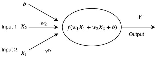
Figure 1.
A single neuron representation with two input features and one output feature Y.
There exists different types of activation function in the literature () defined as follows:
Figure 2 shows the graphical representation of each activation function. In this work, we use as the activation function. In the last decade, Neural Networks have demonstrated a great capability of predicting unseen data from data with complex relationships, therefore, they can be used as a predictive tool for predicting the amount of trade flow between China and its partners along the BRI. In this paper, we follow the implementation details of Wohl and Kennedy [12] and modify the hidden fully connected layers to be as illustrated in Figure 3. Our feedforward network model is made of one input layer, four hidden layers and one output layer. First, The input layer receives information from our dataset called the input feature. Therefore, the number of input nodes in the first layer reflects the number of independent variables in the dataset. In our work, the input feature of the network are the standard gravity model variables such as GDP, distance, border, colonial relationship, trade agreement etc. These input features are summarized in Table 1. No computation is performed in any of the input node. Second, The four hidden layers have no direct connection with the dataset features, but perform computations and transfer information from the input nodes to the output node.
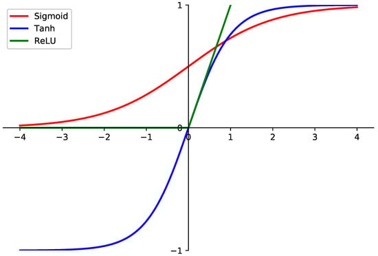
Figure 2.
Graphical representation of the different types of activation functions.
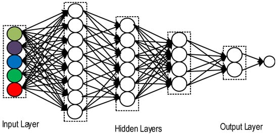
Figure 3.
The Fully Connected Neural Network model used in our paper.

Table 1.
List and description of selected features.
Each node in a hidden layer receives weighted inputs from each node in the input layer. Finally, our output layer gives the result of the computation by the neural network. In this work, the output layer is the predicted amount of bilateral trade between China and its partners along the BRI. In order to train our neural network, we calculate the total error at the output node using Equation (10) and propagate the error back through the network. We use an optimization method called Gradient Descent to adjust all the weights in the network with an aim of reducing the error at the output layer. The network was trained for 100 epoch with a batch size of 16 and a learning rate of .
5. Dataset
5.1. Dataset
The data for this study covers a panel data set of 163 countries from 1990 to 2017. Thus, our data set consists of 4536 observations of bilateral export flows ( country pairs). Various sources of data were used. The data for bilateral trade (exports) is taken from the UN-Comtrade database, GDP (importer, exporter) in billions current U.S. dollars from World Development Indicators (WDI, 2018). Data on location and dummies are indicating contiguity (common border), common language (official language), colony(colonial relationship), was obtained from The Centre d’Etudes Prospectives et d’Informations Internationales (CEPII). The Bilateral distance between China and its partners are taken from CEPII distance database. The Infrastructure index based on Celine and Christopher [31] and Limao and Venables [32] is computed using four variables proxying the Transport infrastructure from the IRF world road statistics and WDI (WB,2018): Total Roads network, total paved Roads, railway network, and number of telephones mainline per person. The model is estimated using China’s bilateral exports between its new silk road partners. Table 1 recapitulates the 13 economic features that are used in our model. Gross domestic product (GDP) and the exports are accounted for in current US $. Most of these features are generally used in the structure of the Gravity Model and consequently are all well-defined.
5.2. Cleaning Techniques
Data cleaning techniques are a common practice and a requirement for many estimators. They are used to avoid deviations in data and potential obstacles in the procedure of prediction. We have applied several data cleansing techniques before we start our analysis. Firstly, we remove all the entries that have no trade flow value as they are not economically significant and cause outlier problems.
Secondly, we extrapolate the missing data using backward and forward linear interpolation. Fourthly, we took the log of data to achieve a smoother distribution of the data as illustrated in Figure 4. After this process, we left with 3936 observations. For the neural network, we standardize the persistent variables (exporter’s GDP, importer’s GDP), scaling them with the goal that their means equal up to zero and their standard deviation equal up to one using Equation (6).
where is mean of the distribution and the standard deviation, both defined as:
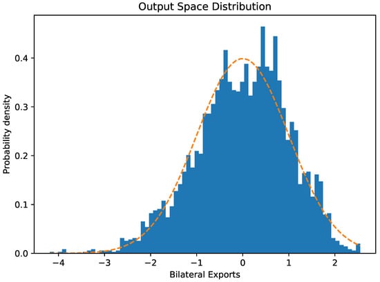
Figure 4.
Histogram of Feature space distribution of bilateral exports.
Table 2 illustrates the descriptive statistics for each variable in the aggregated regions. The average value of China’s bilateral exports for the sample aggregated regions (Asian, Europe, Africa and the rest of the world), 163 countries listed in the Appendix A, is 4.73% with a standard deviation of 2.19%. China is increasingly active in trading with its partners under BRI. The mean value of importer’s GDP and exporter’s GDP for the aggregated regions is respectively 10.14% and 12.34% with a standard deviation of 1.82% and 0.49%. This proves that China’s has a fast-growing economy. In the whole world, China has recently become well-known for its resilient growth and has appeared as the second largest economy in the world after the United States. Therefore, it is not surprising that the average exporter’s GDP, China is higher than that of its trading partners in BRI. The mean of geographical distance between China and its trading partners under BRI is 3.914411 km with a standard deviation 0.2320467 km. The statistics show that importer and exporter transport infrastructure index respectively has average value of 3.854467 ton-km and 5.743929 ton-km with a standard deviation of 0.9630493 ton-km and 0.2032265 ton-km. The maximum value of transport infrastructure index refers to China among its BRI members with 6.228716 ton-km. This is because of China being vigorously occupied with the advancement of infrastructure in accordance with the OBOR initiative [40,45,65,66].
Table 2.
Descriptive Statistics.
The contiguity dummy among countries under BRI has a high mean and standard deviation of 0.068% and 0.25%, respectively. This depicted the fact that countries along the BRI share a few common border trade more than those countries that do not. Of the remaining cultural variables, the mean common official language dummy is 0.025% with a standard deviation of 0.15%. This indicates that common language plays crucial role in BRI trading partners. Culture could decidedly correlated with an expansion in trade flows or not. This is in line with the aspiration that culture influences on trade [44,67,68]. The average performance of colony dummy in the studied countries amounted to 0.0246% with a standard deviation of 0%. This shows that colonial link is less important in BRI program, on average, null. The average performance of Regional trade agreements dummy (obor, asean, eac and sadc) in the BRI trading partners amounted to 0.46%, 0.94%, 0.97% and 0.97% with a standard deviation of 0.50%, 0.24%, 0.17% and 0.27%, respectively. The highest Regional trade agreements indicator performance was 0.50% among BRI partners, while the lowest was 0.17% in East Africa community. BRI looks to develop regional integration by improving infrastructure and strengthening trade. This is in line with the aspiration that BRI boost regional integration in improving economic growth between its trading partners [41,65,69,70].
6. Evaluation Results and Analysis
In this section; we formally evaluate the two models and present comparative results.
6.1. Evaluation Metrics
To compare the predictive performance of our neural network model against gravity model. It is useful to quantify the performance with pre-defined metrics. From the regression problem, the commonly used metrics are a mean square error. In this work, we use , known as the coefficient of determination and mean square error (MSE) as our metrics.
6.1.1. Coefficient of Determination
The coefficient of determination R2 portrays how great our model is at making expectations: it speaks to the extent of the variance in the dependent variable Trade export flow that is predictable from the independent feature space variables. It is generally characterized as:
where is the residual sum of squares, the total sum of square or the proportion to the variance of the data, the input vector associated with a predicted value and the mean of the observed data. To avoid division by zero, we modify Equation (8) to produce:
where is an empiric parameter which value was set to . ranges from 0 to 1: If , the model always fails to predict the target variable, and if the model perfectly predicts the target variable. Any value between 0 and 1 indicates what percentage of the target variable, using the model, can be explained by the features. If it indicates that the model is no better than one that constantly predicts the mean of the target variable.
6.1.2. Mean-Square-Error (MSE)
The loss function (MSE) is used to indicate how far our predictions deviate from the target. During the training phase, the weights are updated based on this quantity. While the network is training, the loss function is decreasing as illustrated in Figure 5. MSE is defined as:
where is the actual observation, the predicted observation and N is the number of observations. We also show root mean squared error RMSE as it is frequently used to gauge the contrasts between values anticipated by a model or an estimator and the values observed. Root mean square error is mostly characterized as the square root of differences between predicted values and observed values, i.e., of the mean square . It is a very frequently used measure of the differences between value predicted value by an estimator or a model and the actual observed values. It is a good measure of accuracy which is used in order to perform comparison forecasting errors from different estimators for a certain variable, but not among the variables, since this measure is scale dependent.
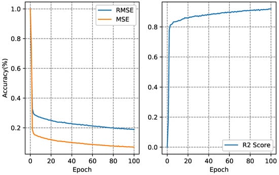
Figure 5.
Mean Squared Error, Root Mean Squared Error and R2 plotted over 100 epochs.
6.2. Analysis and Predictions
Table 3 shows the results of the evaluations. For the baseline dataset, the OLS estimator has an out-of-sample root Mean squared error of $16.05 billion, the PPML estimator has an out-of-sample RMSE of $6.53 billion, and the neural network has an out-of-sample RMSE of $3.83 billion. For the dataset with country fixed effects, the OLS estimator has an out-of-sample RMSE of $11.30 billion, the PPML estimator has an out-of-sample RMSE of $9.79 billion, and the neural network has an out-of-sample RMSE of $1.91 billion. For the dataset with country-year fixed effects, the OLS estimator has an out-of-sample RMSE of $6.66 billion, and the PPML has an out-of-sample RMSE of $8.17 billion, and the neural network has an out-of-sample RMSE of $1.89 billion. These analyses were repeated several times, allowing for variation in the random training-test division and the development of the neural network, and these outcomes are representative.
Table 3.
Trade Predictions using different Estimators (in millions US $).
To illustrate forecasting application of our model, we trained the neural network on the full dataset with country fixed from 1990 to 2012 and used it to predict bilateral trade export between China and its major trading partners in the Silk and Road Initiative. The estimation covers the period from 2013 to 2017. We furnished the neural network with the actual GDP’s of China and its BRI partners. Table 4 shows the results of the predictions. The neural network’s estimations are sensibly close to actual trade values even 5 years beyond the training period. For instance, the neural network model predicted trade flow value for Kenya in 2013 which is close by to the actual value . Also, similar results can be found on Burundi, Rwanda, Tanzania, Uganda and Djibouti trade flow predictions for the same year. Moreover, we observe that the neural network model still makes a good prediction for the year 2017 which is far from the value the network was trained on. Prediction results are shown in Figure 6. The x-axis represents the years and the y-axis is the value of bilateral exports amount in US $.
Table 4.
Neural network predictions versus actual trade values in millions US $.
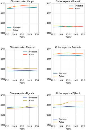
Figure 6.
Neural network predictions versus actual trade.
7. Conclusions
We have investigated the relative predictive powers of the neural network analysis and the gravity models. Results based on the analysis and comparison have demonstrated the ability of the neural network to predict efficiently and more effectively the bilateral trade flow using other economic variables. This is based on its capacity to capture nonlinear interactions between features. The neural network is also able to improve the prediction of the Gravity Model performance by a test set R2 score of 0.15, using the same set of features. This will be a useful aid to policymakers, analysts and firms engaged in the international trade business and provide impetus for all players in the industry to gauge the effects of this trade collaboration. The influence and sustainability of the BRI programme will heavily rely on the benefits that the partner countries derive from such arrangements. The estimation of these trades using the neural network model offers one of many ways by which partner countries can measure its impact and possible sustainability of such partnership.
Author Contributions
K.D. and L.Y. conceptualized the model and designed the methodology, K.D. conducted the formal analysis and the first investigation, K.D. collected the dataset and wrote the first draft, L.Y. reviewed the paper, the editing and conducted the project supervision. K.D. and L.Y. wrote the final manuscript for submission.
Acknowledgments
We appreciate Jean-Paul Ainam, Charles Essel, Curtis Lartey and Benjamin Klugah-Brown for their useful contributions. We are also very grateful to Ma Yongkai for his expert advices and helpful suggestions throughout the manuscript.
Conflicts of Interest
The authors declare no conflict of interest.
Abbreviations
The following abbreviations are used in this manuscript:
| BRI | Belt and Road Initiative |
| PPML | Poisson pseudo-maximum likelihood |
| NNA | Neural Networks analysis |
| GDP | Gross Domestic Product |
| RMSE | Out-of-sample root mean squared error |
| Obs. | Observations |
| Std.Dev. | Standard Deviation |
| Min. | Minimum |
| Max. | Maximum |
Appendix A
Table A1.
List of country names in entire sample.
Table A1.
List of country names in entire sample.
| Albania | Algeria | Andorra | Angola | Argentina |
| Armenia | Australia | Austria | Azerbaijan | Bahamas |
| Bangladesh | Belarus | Belgium | Belize | Benin |
| Bermuda | Bhutan | Bolivia | Bosnia & Herzegovina | Botswana |
| Brazil | Brunei Darussalam | Saudi Arabia | Liberia | Dominican Republic |
| Ireland | Bulgaria | Senegal | Libya | Ecuador |
| Israel | Burkina Faso | Sierra Leone | Lithuania | Egypt |
| Italy | Burundi | Singapore | Luxembourg | Equatorial Guinea |
| Jamaica | Cambodia | Slovak Republic | Macedonia | Eritrea |
| Japan | Cameroon | Slovenia | Madagascar | Estonia |
| Jordan | Canada | Somalia | Malawi | Ethiopia |
| Kazakhstan | Cabo Verde | South Africa | Malaysia | Fiji |
| Kenya | Central African Rep. | Spain | Maldives | Finland |
| Korea, Dem. People’s Rep. | Chad | Sri Lanka | Mali | France |
| Korea, Rep. | Chile | Sudan | Malta | Gabon |
| Kuwait | China | Swaziland | Mauritania | Gambia |
| Kyrgyz Republic | Colombia | Sweden | Mauritius | Georgia |
| Lao PDR | Comoros | Switzerland | Mexico | Germany |
| Latvia | Congo, Dem. Rep. | Tajikistan | Moldova | Ghana |
| Lebanon | Congo, Rep. | Tanzania | Mongolia | Greece |
| Lesotho | Costa Rica | Uganda | Morocco | Guinea |
| Nigeria | Cote d’Ivoire | Ukraine | Mozambique | Guinea-Bissau |
| Norway | Croatia | United Arab Emirates | Myanmar | Honduras |
| Oman | Cuba | United Kingdom | Namibia | Hungary |
| Pakistan | Cyprus | United States | Nepal | Iceland |
| Panama | Czech Republic | Uruguay | Netherlands | India |
| Paraguay | Denmark | Uzbekistan | New Zealand | Indonesia |
| Peru | Djibouti | Vanuatu | Nicaragua | Iran, Islamic Rep. |
| Philippines | Dominica | Venezuela, RB | Niger | Iraq |
| Poland | Thailand | Vietnam | Romania | Turkey |
| Portugal | Togo | Yemen, Rep. | Russian Federation | Turkmenistan |
| Puerto Rico | Trinidad and Tobago | Zambia | Rwanda | Tuvalu |
| Qatar | Tunisia | Zimbabwe |
Table A2.
List of OBOR country names in entire sample.
Table A2.
List of OBOR country names in entire sample.
| Albania | Egypt | Kuwait | Nepal | Sweden |
| Armenia | Estonia | Kyrgyz Republic | Netherlands | Switzerland |
| Austria | Ethiopia | Lao PDR | Norway | Tajikistan |
| Azerbaijan | Finland | Latvia | Oman | Tanzania |
| Bangladesh | France | Lebanon | Pakistan | Thailand |
| Belarus | Germany | Lithuania | Philippines | Tunisia |
| Belgium | Greece | Luxembourg | Poland | Turkey |
| Bhutan | Guinea | Macedonia Portugal | Turkmenistan | |
| Bosnia and Herzegovina | Hungary | Madagascar | Qatar | Uganda |
| Brunei Darussalam | Iceland Malaysia | Romania | Ukraine | |
| Bulgaria | India | Maldives | Russian Federation | United Kingdom |
| Burundi | Indonesia | Malta | Rwanda | Uzbekistan |
| Cambodia | Iran | Mauritania | Saudi Arabia | Zambia |
| China | Iraq | Mauritius | Singapore | Zimbabwe |
| Croatia | Ireland | Moldova | Slovak Republic | South Africa |
| Czech Republic | Israel | Mongolia | Slovenia | Spain |
| Denmark | Italy | Morocco | Somalia | Sri Lanka |
| Djibouti | Jordan | Mozambique | Kazakhstan | Sudan |
| Myanmar | Kenya |
Table A3.
List of country used for Asia, Europe, America and Africa.
Table A3.
List of country used for Asia, Europe, America and Africa.
| Asia | ||||
| Bangladesh | Lao PDR | Armenia | Thailand | Sri Lanka |
| Bhutan | Malaysia | Azerbaijan | Vietnam | Taiwan |
| Brunei Darussalam | Maldives | Belarus | Estonia | Tajikistan |
| Burma | Mongolia | Georgia | Latvia | Turkmenistan |
| Cambodia | Nepal | Kazakhstan | Lithuania | Ukraine |
| China | Pakistan | Kyrgyzstan | Iran | Korea, Rep. |
| India | Philippines | Moldova | Japan | Oman |
| Indonesia | Singapore | Russia federation | Korea, Dem. People’s Rep. | Saudi Arabia |
| Yemen, Rep. | Qatar | Indonesia | United Arab Emirates | Myanmar |
| Europe | ||||
| Albania | Finland | Macedonia, FYR | Croatia | Italy |
| Andorra | France | Malta | Czech Republic | Latvia |
| Austria | Germany | Moldova | Denmark | Lithuania |
| Belarus | Greece | Netherlands | Estonia | Luxembourg |
| Belgium | Hungary | Norway | Romania | Slovenia |
| Bosnia and Herzegovina | Iceland | Poland | Russian Federation | Spain |
| Bulgaria | Ireland | Portugal | Slovak Republic | Sweden |
| Switzerland | Ukraine | United | Kingdom | |
| America | ||||
| Bermuda | Bolivia | Chile | United States | Puerto Rico |
| Brazil | Venezuela, RB | Costa Rica | Panama | Paraguay |
| Canada | Colombia | Cuba | Jamaica | Ecuador |
| Peru | Argentina | Uruguay Mexico | Dominican Republic | |
| Honduras | Nicaragua | Bahamas | Dominica | Belize |
| Africa | ||||
| Angola | Ghana | Rwanda | Mozambique | Tanzania |
| Burundi | Guinea | Sudan | Mauritania | Uganda |
| Benin | Gambia | Senegal | Mauritius | South Africa |
| Burkina Faso | Guinea-Bissau | Sierra Leone | Malawi | Zambia |
| Botswana | Equatorial Guinea | Somalia | Namibia | Zimbabwe |
| Central African Republic | Kenya | South Sudan | Niger | Comoros |
| Cote d’Ivoire | Liberia | Sao Tome and Principe | Nigeria | Cabo Verde |
| Cameroon | Lesotho | Swaziland | Togo | Eritrea |
| Congo, Dem. Rep. | Madagascar | Chad | Gabon | Ethiopia |
| Congo, Rep. | Mali | |||
References
- Huang, Y. Understanding China’s Belt & Road Initiative: Motivation, framework and assessment. China Econ. Rev. 2016, 40, 314–321. [Google Scholar]
- Liu, W.; Dunford, M. Inclusive globalization: Unpacking China’s belt and road initiative. Area Dev. Policy 2016, 1, 323–340. [Google Scholar] [CrossRef]
- Swaine, M.D. Chinese views and commentary on the ‘One Belt, One Road’initiative. China Leadership Monit. 2015, 47, 3. [Google Scholar]
- Johnston, L.A. The Belt and Road Initiative: What is in it for China? Asia Pac. Policy Stud. 2019, 6, 40–58. [Google Scholar] [CrossRef]
- Daily, C. Xi Opens ’Project of the Century’ with Keynote Speech. 2017. Available online: http://www.chinadaily.com.cn/beltandroadinitiative/2017-05/14/content_29337406.htm (accessed on 15 February 2018).
- SCMP. Belt and Road: The Projects. 2017. Available online: https:/www.scmp.com/news/china/economy/article/2099973/belt-and-road-projects-china-doesnt-want-anyone-talking-about (accessed on 10 February 2019).
- Valentin, A.; Spangenberg, J.H. A guide to community sustainability indicators. Environ. Impact Assess. Rev. 2000, 20, 381–392. [Google Scholar] [CrossRef]
- Isard, W. Location Theory and Trade Theory: Short-Run Analysis. Q. J. Econ. 1954, 68, 305–320. [Google Scholar] [CrossRef]
- Tinbergen, J. Shaping the world economy: Suggestions for an international economic policy. Econ. J. 1966, 76, 92–95. [Google Scholar]
- Pöyhönen, P. A Tentative Model for the Volume of Trade between Countries. Weltwirtsch. Arch. 1963, 90, 93–100. [Google Scholar]
- Varian, H.R. Big Data: New Tricks for Econometrics. J. Econ. Perspect. 2014, 28, 3–28. [Google Scholar] [CrossRef]
- Wohl, I.; Kennedy, J. Neural Network Analysis of International Trade; U.S. International Trade Commission: Washington, DC, USA, 2018.
- Nummelin, T.; Hänninen, R. Model for international trade of sawnwood using machine learning models. Nat. Resour. Bioecon. Stud. 2016, 74. [Google Scholar] [CrossRef]
- Elif, N. Estimating and Forecasting Trade Flows by Panel Data Analysis and Neural Networks. J. Facul. Econ. 2014, 64, 85–111. [Google Scholar]
- Tkacz, G.; Hu, S. Forecasting GDP Growth Using Artificial Neural Networks; Bank of Canada: Ottawa, ON, Canada, 1999. [Google Scholar]
- Gradojevic, N.; Yang, J. The Application of Artificial Neural Networks to Exchange Rate Forecasting: The Role of Market Microstructure Variables; Bank of Canada: Ottawa, ON, Canada, 2000. [Google Scholar]
- Sonia Circlaeys, C.K.; Kumazawa, D. Bilateral Trade Flow Prediction; Stanford Final Reports; Semantic Scholar: California, CA, USA, 2017. [Google Scholar]
- Bajari, P.; Nekipelov, D.; Ryan, S.P.; Yang, M. Machine Learning Methods for Demand Estimation. Am. Econ. Rev. 2015, 105, 481–485. [Google Scholar] [CrossRef]
- Beverelli, C.; Keck, A.; Larch, M.; Yotov, Y. Institutions, Trade and Development: A Quantitative Analysis; EconStor: Munich, Germany, 2018; Available online: http://hdl.handle.net/10419/176939 (accessed on 8 March 2019).
- Lu, H.; Rohr, C.; Hafner, M.; Knack, A. China Belt and Road Initiative: Measuring the Impact of Improving Transport Connectivity on Trade in the Region—A Proof-Of-Concept Study; RAND: Cambridge, UK, 2018. [Google Scholar]
- Herrero, A.G.; Xu, J. China’s Belt and Road Initiative: Can Europe Expect Trade Gains? China World Econ. 2017, 25, 84–99. [Google Scholar] [CrossRef]
- Fiorentini, R.; Verashchagina, A. Immigration and Trade: The Case Study of Veneto Region in Italy; AIEAA Conference: Piacenza, Italy, 2017. [Google Scholar]
- Anderson, J.; van Wincoop, E. Gravity with Gravitas: A Solution to the Border Puzzle. Am. Econ. Rev. 2003, 93, 170–192. [Google Scholar] [CrossRef]
- Baier, S.L.; Bergstrand, J.H. Bonus vetus OLS: A simple method for approximating international trade-cost effects using the gravity equation. J. Int. Econ. 2009, 77, 77–85. [Google Scholar] [CrossRef]
- Du, J.; Zhang, Y. Does One Belt One Road initiative promote Chinese overseas direct investment? China Econ. Rev. 2018, 47, 189–205. [Google Scholar] [CrossRef]
- Piermartini, R.; Yotov, Y. Estimating Trade Policy Effects with Structural Gravity; EconStor: Munich, Germany, 2016. [Google Scholar]
- Athey, S. The Impact of Machine Learning on Economics; University of Chicago Press: Chicago, CA, USA, 2018. [Google Scholar]
- Tillema, F.; Van Zuilekom, K.M.; Van Maarseveen, M.F. Comparison of neural networks and gravity models in trip distribution. Comput. Aided Civ. Infrastruct. Eng. 2006, 21, 104–119. [Google Scholar] [CrossRef]
- Pourebrahim, N.; Sultana, S.; Thill, J.C.; Mohanty, S. Enhancing Trip Distribution Prediction with Twitter Data: Comparison of Neural Network and Gravity Models; ACM: New York, NY, USA, 2018; pp. 5–8. [Google Scholar]
- Alaloul, W.S.; Liew, M.S.; Wan Zawawi, N.A.; Mohammed, B.S.; Adamu, M. An Artificial neural networks (ANN) model for evaluating construction project performance based on coordination factors. Cogent Eng. 2018, 5, 1–18. [Google Scholar] [CrossRef]
- Celine, C.; Christopher, G. Landlockedness, Infrastructure and Trade: New Estimates for Central Asian Countries. Cerdi Pap. 2008, 1. [Google Scholar] [CrossRef]
- Limao, N.; Venables, A.J. Infrastructure, geographical disadvantage, transport costs, and trade. World Bank Econ. Rev. 2001, 15, 451–479. [Google Scholar] [CrossRef]
- Konings, J. Trade Impacts of the Belt and Road Initiative; Think: London, UK, 2018. [Google Scholar]
- Liu, X.; Zhang, K.; Chen, B.; Zhou, J.; Miao, L. Analysis of logistics service supply chain for the One Belt and One Road initiative of China. Transp. Res. Part E Logist. Transp. Rev. 2018, 117, 23–39. [Google Scholar] [CrossRef]
- Chen, S.C.; Hou, J.; Xiao, D. “One Belt, One Road” Initiative to Stimulate Trade in China: A Counter-Factual Analysis. Sustainability 2018, 10, 3242. [Google Scholar] [CrossRef]
- Ye, J.; Haasis, H.D. Impacts of the BRI on International Logistics Network; Springer Cham: New York, NY, USA, 2018; pp. 250–254. [Google Scholar]
- Hayes, N. The Impact of China’S One Belt One Road Initiative on Developing Countries; LSE: London, UK, 2017. [Google Scholar]
- Bartley Johns, M.; Clarke, J.L.; Kerswell, C.; McLinden, G. Trade Facilitation Challenges and Reform Priorities for Maximizing the Impact of the Belt and Road Initiative; World Bank: Washington, DC, USA, 2018. [Google Scholar]
- Fardella, E.; Prodi, G. The Belt and Road Initiative Impact on Europe: An Italian Perspective. China World Econ. 2017, 25, 125–138. [Google Scholar] [CrossRef]
- Zhai, F. China’s belt and road initiative: A preliminary quantitative assessment. J. Asian Econ. 2018, 55, 84–92. [Google Scholar] [CrossRef]
- De Soyres, F.; Mulabdic, A.; Murray, S.; Rocha, N.; Ruta, M. How Much Will the Belt and Road Initiative Reduce Trade Costs? World Bank: Washington, DC, USA, 2018. [Google Scholar]
- Yii, K.J.; Bee, K.Y.; Cheam, W.Y.; Chong, Y.L.; Lee, C.M. Is Transportation Infrastructure Important to the One Belt One Road (OBOR) Initiative? Empirical Evidence from the Selected Asian Countries. Sustainability 2018, 10, 4131. [Google Scholar] [CrossRef]
- Boffa, M. Trade Linkages Between the Belt and Road Economies (English); Policy Research Working Paper; No. WPS 8423; World Bank: Washington, DC, USA, 2018. [Google Scholar]
- Liu, A.; Lu, C.; Wang, Z. The roles of cultural and institutional distance in international trade: Evidence from China’s trade with the Belt and Road countries. China Econ. Rev. 2018. [Google Scholar] [CrossRef]
- Liu, B. The Role of Chinese Financial Institutions in Promoting Sustainable Investment under the One Belt One Road Initiative; APDR Working Paper No. 18-7; SSRN Electronic Journal: Vancouver, BC, Canada, 2018. [Google Scholar]
- World Bank. Belt and Road Initiative; World Bank: Ottawa, ON, Canada, 2018. [Google Scholar]
- Yotov, Y.V. A simple solution to the distance puzzle in international trade. Econ. Lett. 2012, 117, 794–798. [Google Scholar] [CrossRef]
- Eichengreen, B.; Irwin, D.A. Trade blocs, currency blocs and the reorientation of world trade in the 1930s. J. Int. Econ. 1995, 38, 1–24. [Google Scholar] [CrossRef]
- Head, K.; Mayer, T. What separates us? Sources of resistance to globalization. Can. J. Econ. 2013, 46, 1196–1231. [Google Scholar] [CrossRef]
- Silva, J.M.C.S.; Tenreyro, S. The Log of Gravity. Rev. Econ. Stat. 2006, 88, 641–658. [Google Scholar] [CrossRef]
- Herbrich, R.; Keilbach, M.; Graepel, T.; Bollmann-Sdorra, P.; Obermayer, K. Neural Networks in Economics; Springer: Boston, MA, USA, 1999; pp. 169–196. [Google Scholar]
- Cao, W.; Mirjalili, V.; Raschka, S. Consistent Rank Logits for Ordinal Regression with Convolutional Neural Networks. arXiv, 2019; arXiv:1901.07884. [Google Scholar]
- Hassani, H.; Silva, E.S. Forecasting UK consumer price inflation using inflation forecasts. Res. Econ. 2018, 72, 367–378. [Google Scholar] [CrossRef]
- Rasool, S.A.; Kiani, A.K. Stock Returns Prediction by using Artificial Neural Network Model for Pakistan Stock Exchange. Sarhad J. Manag. Sci. 2018, 4, 192–204. [Google Scholar]
- Naderi, M.; Khamehchi, E.; Karimi, B. Novel statistical forecasting models for crude oil price, gas price, and interest rate based on meta-heuristic bat algorithm. J. Petrol. Sci. Eng. 2019, 172, 13–22. [Google Scholar] [CrossRef]
- Moshiri, S.; Cameron, N. Neural network versus econometric models in forecasting inflation. J. Forecast. 2000, 19, 201–217. [Google Scholar] [CrossRef]
- Rana, M.S.; Zahan, S. Data Prediction from a Set of Sampled Data Using Artificial Neural Network in Matlab Simulink; WJPR: New Delhi, India, 2018. [Google Scholar]
- Chen, J. Neural Network Applications in Agricultural Economics; University of Kentucky, UKnowledge: Kentucky, KY, USA, 2005. [Google Scholar]
- Hegde, N.G.; Mujumdar, S.; Jambarmath, S.S.; Madhavi, R. Survey paper on Agriculture Yield Prediction Tool using Machine Learning. Int. J. 2017, 5, 36–39. [Google Scholar]
- Alwosheel, A.; van Cranenburgh, S.; Chorus, C.G. Is your dataset big enough? Sample size requirements when using artificial neural networks for discrete choice analysis. J. Choice Model. 2018, 28, 167–182. [Google Scholar] [CrossRef]
- Bernardes, P.A. Imputação e Estudos Genômicos de Bovinos Nelore; Universidade Estadual Paulista (UNESP): Sao Paolo, Brazil, 2018. [Google Scholar]
- De Palacios, P.; Fernández, F.G.; García-Iruela, A.; González-Rodrigo, B.; Esteban, L.G. Study of the influence of the physical properties of particleboard type P2 on the internal bond of panels using artificial neural networks. Comput. Electron. Agric. 2018, 155, 142–149. [Google Scholar] [CrossRef]
- Pérez-Sánchez, B.; Fontenla-Romero, O.; Guijarro-Berdiñas, B. A review of adaptive online learning for artificial neural networks. Artif. Intell. Rev. 2018, 49, 281–299. [Google Scholar] [CrossRef]
- Tamara, G.; Peter, H.; Serge, S.; Ricky, U. Extending The Cepii Gravity Data Set; U.S. International Trade Commission: Washington, DC, USA, 2017.
- Wong, K.Y. The “Belt and Road” Initiative and Economic Integration; Springer: Gateway East, Singapore, 2017; pp. 59–86. [Google Scholar]
- Zhang, J.; Wu, Z. Effects of Trade Facilitation Measures on Trade between China and Countries along the Belt and Road Initiative; Springer International Publishing: New York, NY, USA, 2018; pp. 227–241. [Google Scholar]
- Tadesse, B.; White, R.; Zhongwen, H. Does China’s trade defy cultural barriers? Int. Rev. Appl. Econ. 2017, 31, 398–428. [Google Scholar] [CrossRef]
- Hanousek, J.; Kočenda, E. Factors of trade in Europe. Econ. Syst. 2014, 38, 518–535. [Google Scholar] [CrossRef]
- Maria, V. Regional Trade Agreements, Integration and Development; Unctad: Geneva, Switzerland, 2017. [Google Scholar]
- Koh, S.G.; Kwok, A.O. Regional integration in Central Asia: Rediscovering the Silk Road. Tour. Manag. Perspect. 2017, 22, 64–66. [Google Scholar] [CrossRef]
© 2019 by the authors. Licensee MDPI, Basel, Switzerland. This article is an open access article distributed under the terms and conditions of the Creative Commons Attribution (CC BY) license (http://creativecommons.org/licenses/by/4.0/).