Solar Energy Production for a Decarbonization Scenario in Spain


Abstract
1. Introduction
2. Materials and Methods
2.1. Stationary Forecasting Models
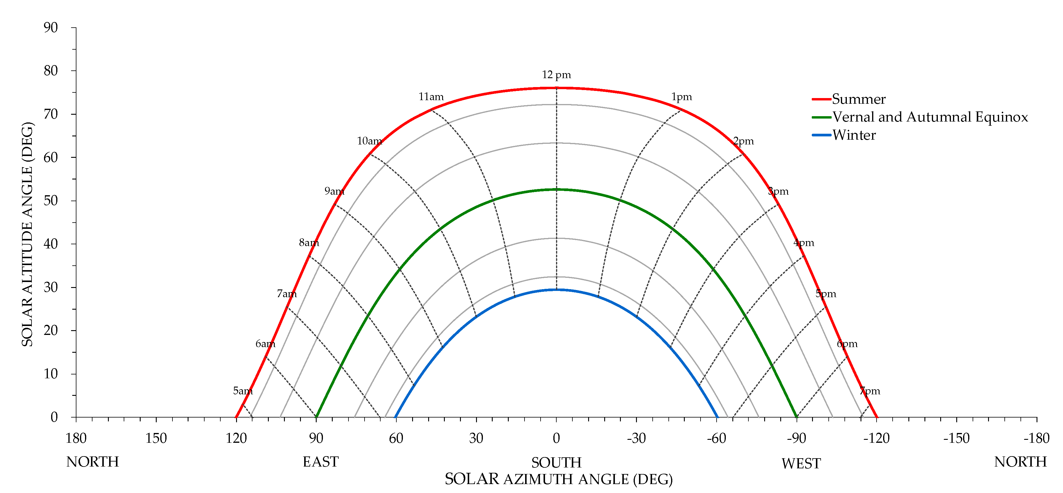
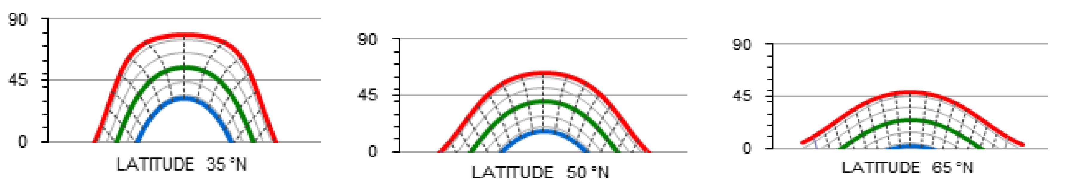
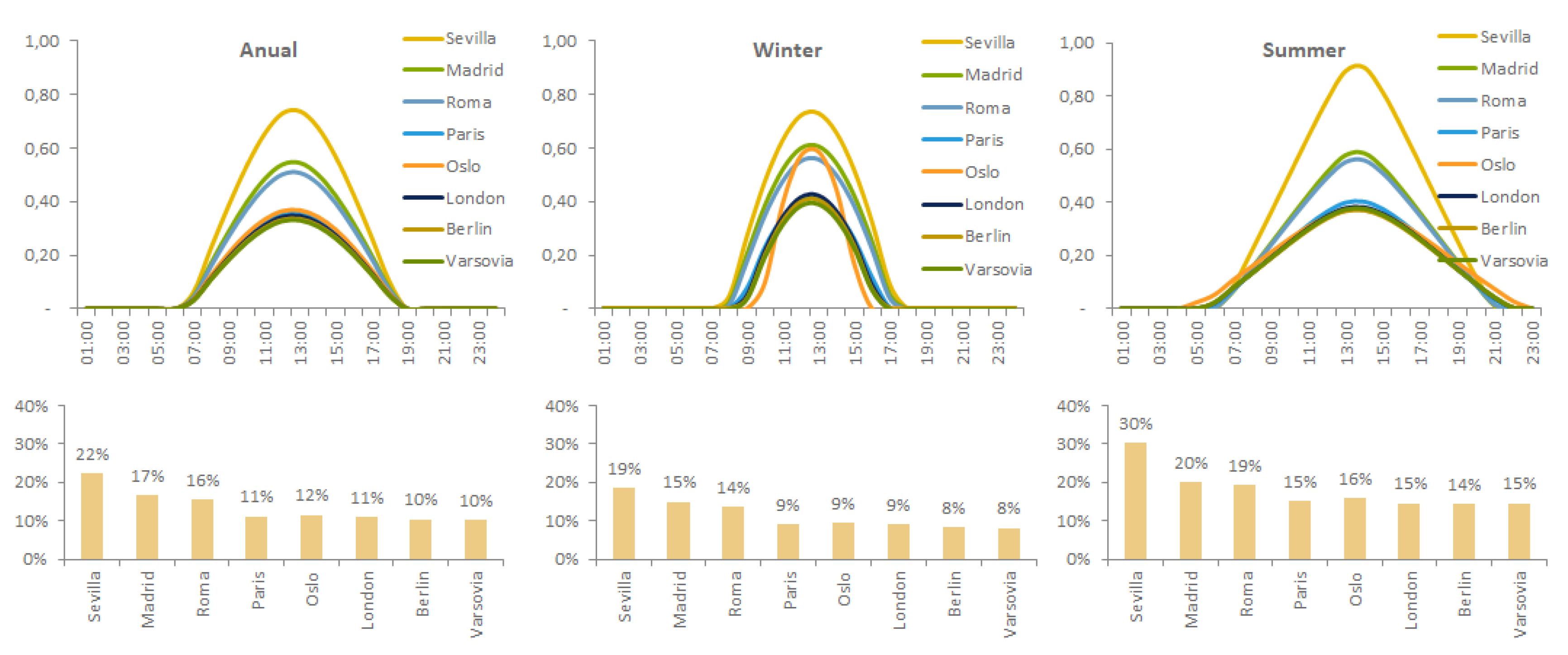
2.2. The Sun as a Renewable Electricity Source
2.3. Case Study: Spain
3. Results
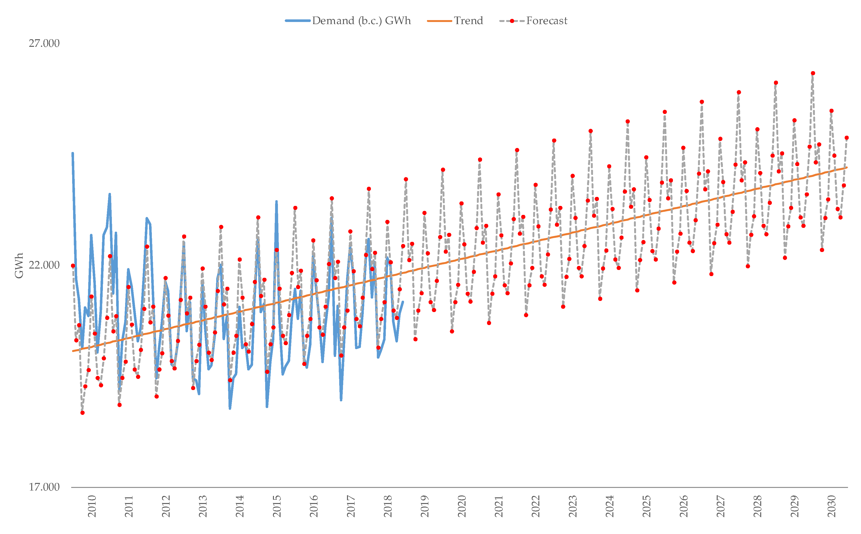
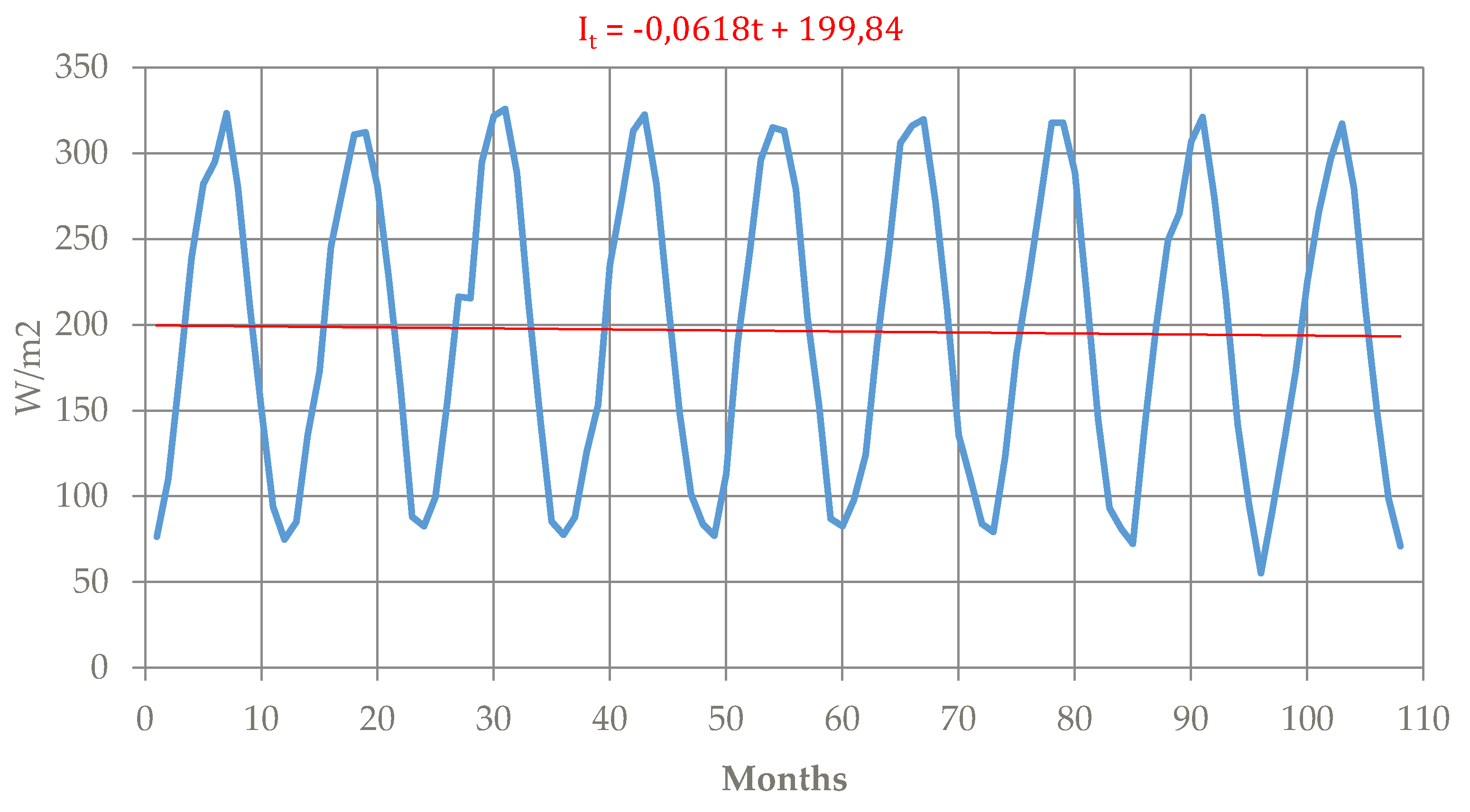
3.1. Linear Trend
- , irradiation ( period or later);
- , intersection of axis;
- , slope;
- , temporal period under study;
- , average of current periods;
- , current observation;
- , average of current parameters.
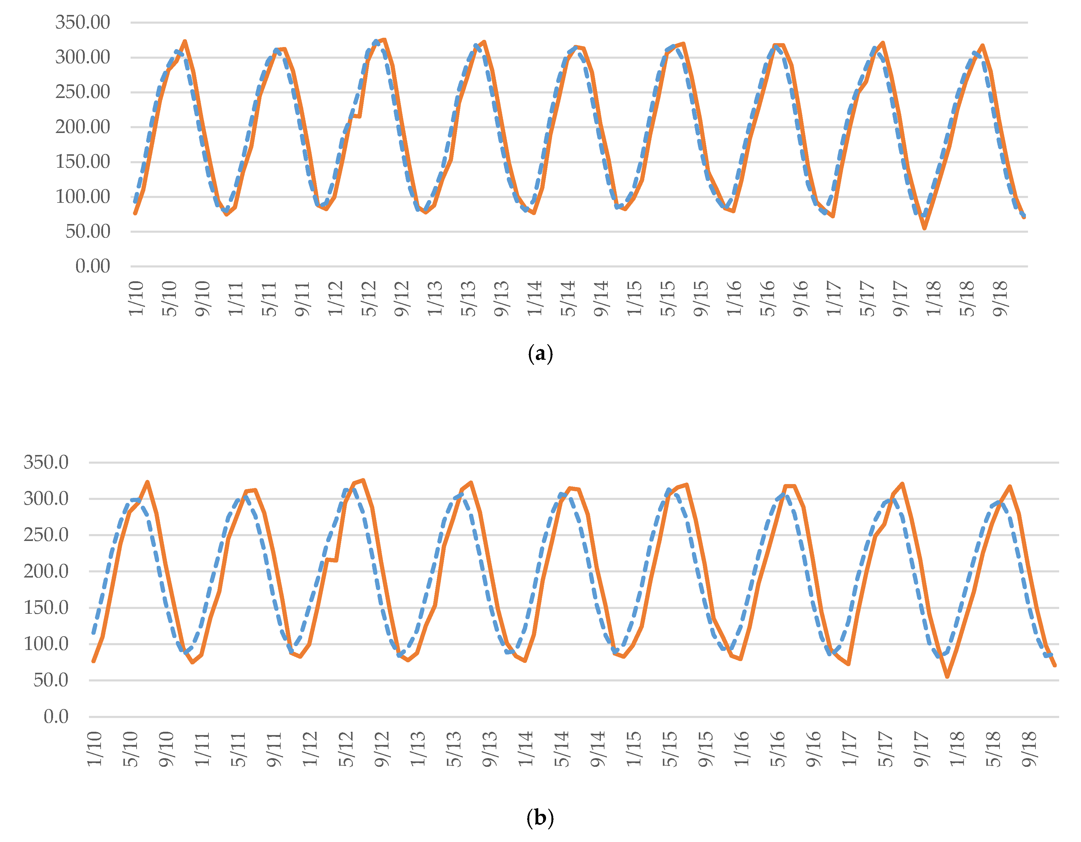
3.2. Simple or Weighted Moving Average
- , number of periods;
- , weight ;
- , irradiation ( period or later);
- number of periods to average;
- , temporal period under study;
- average of current periods;
- current observation;
- current observation ( period).
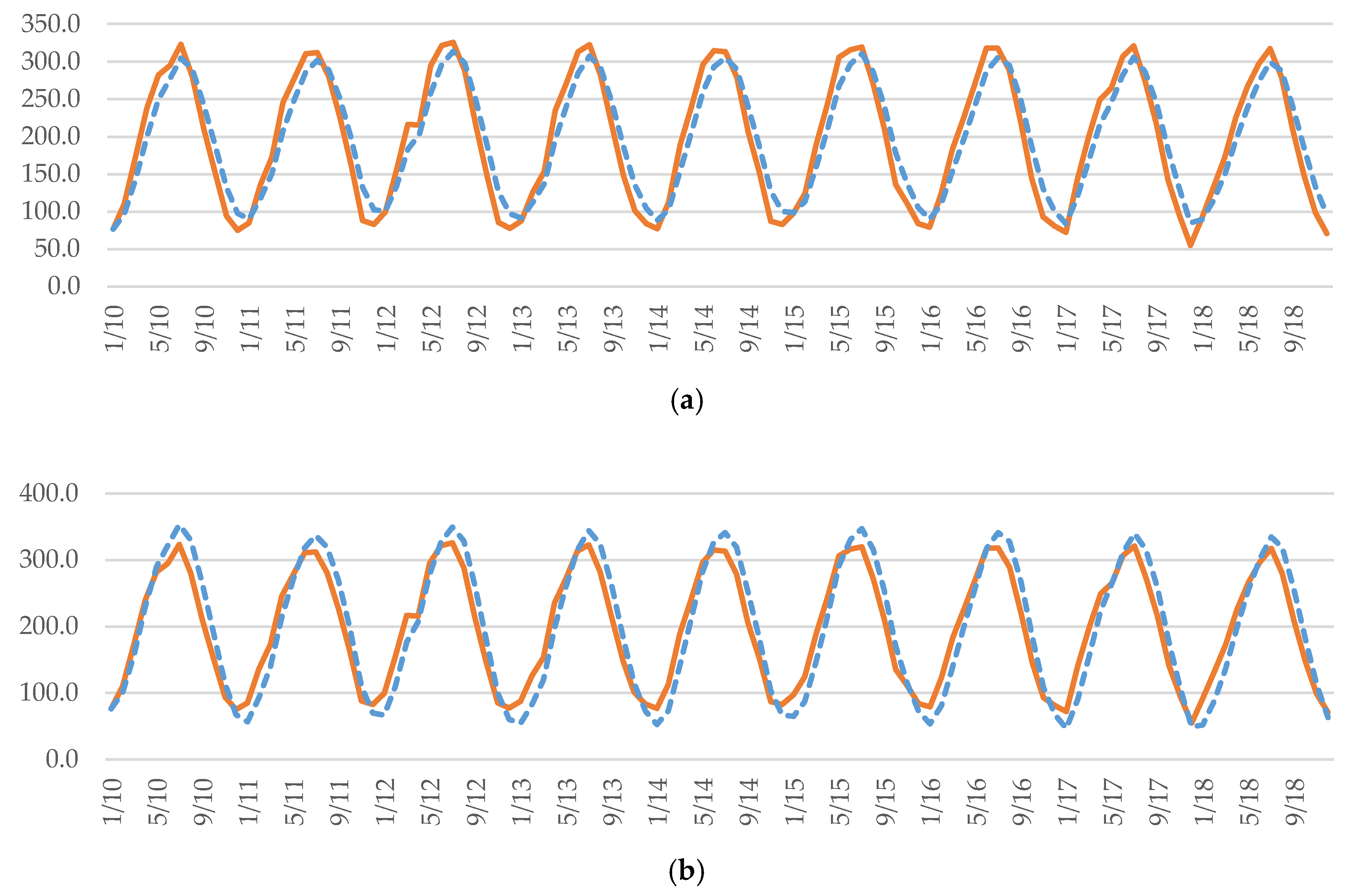
3.3. Simple or Adjusted Exponential Smoothing (Double Exponential or Holt–Winters Method)
- , irradiation ( period or later);
- , irradiation ( period or later);
- , current observation ( period);
- , smoothing coefficient.
- , trend with exponential smooth ( last period);
- Model Included Trend ( last period).
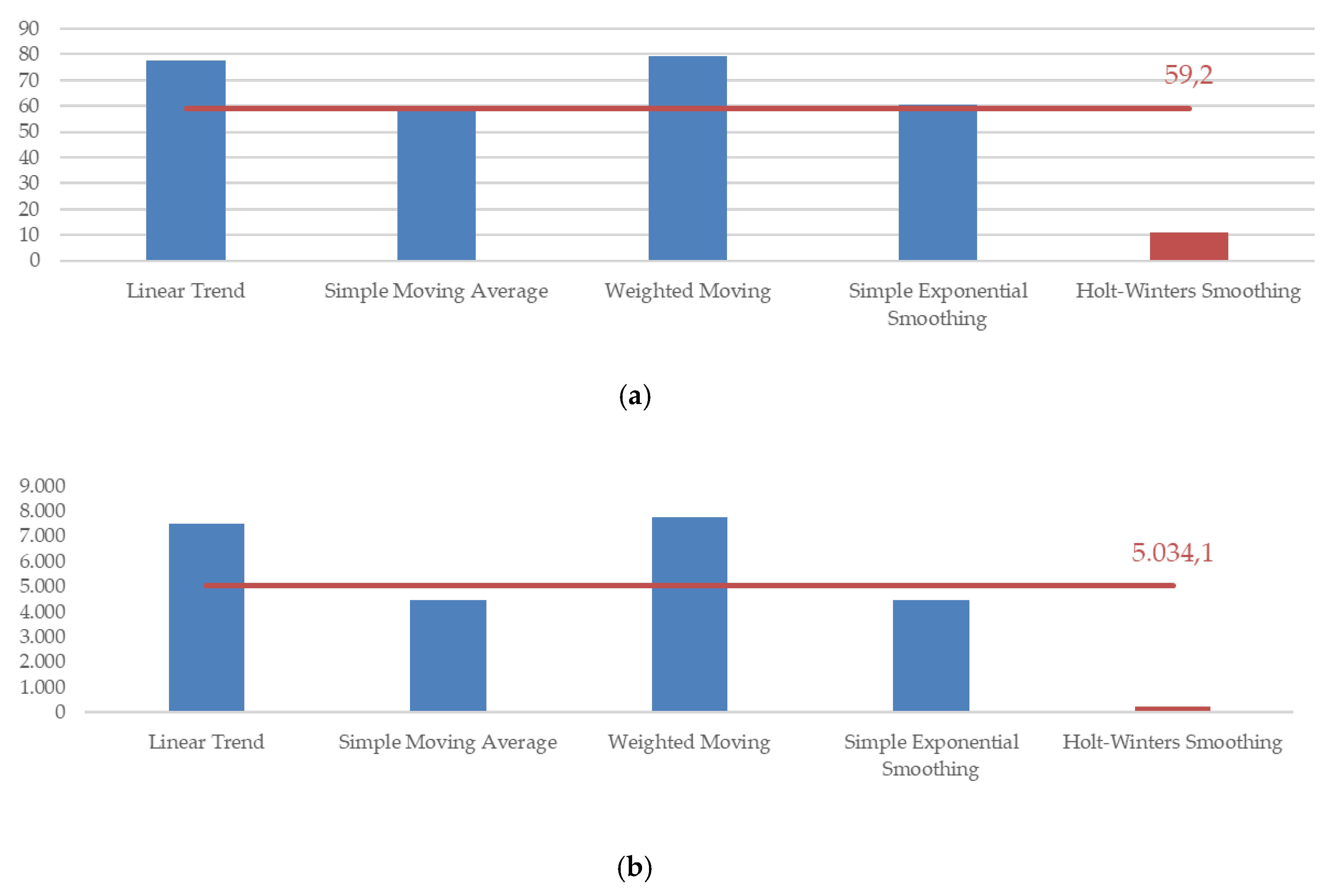
3.4. Comparison of the Different Techniques
4. Discussion
5. Conclusions
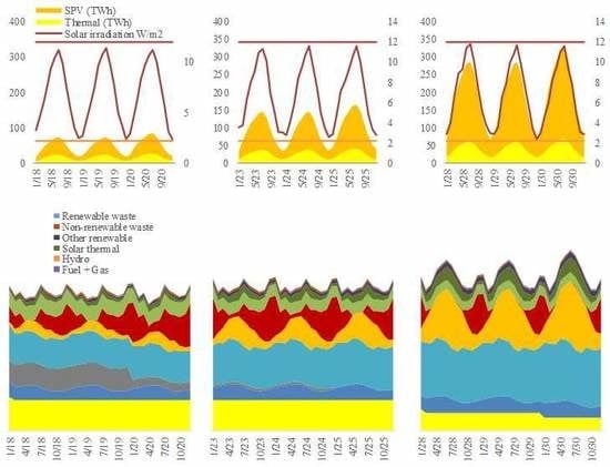
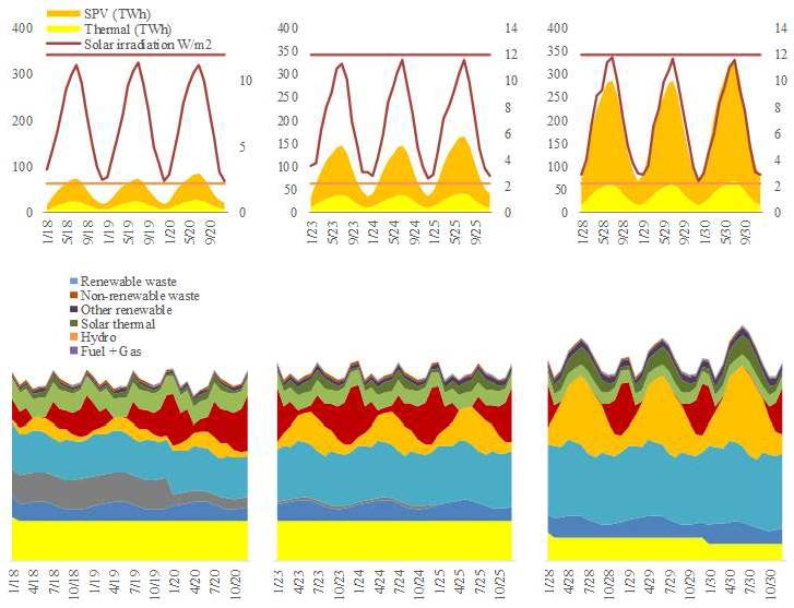
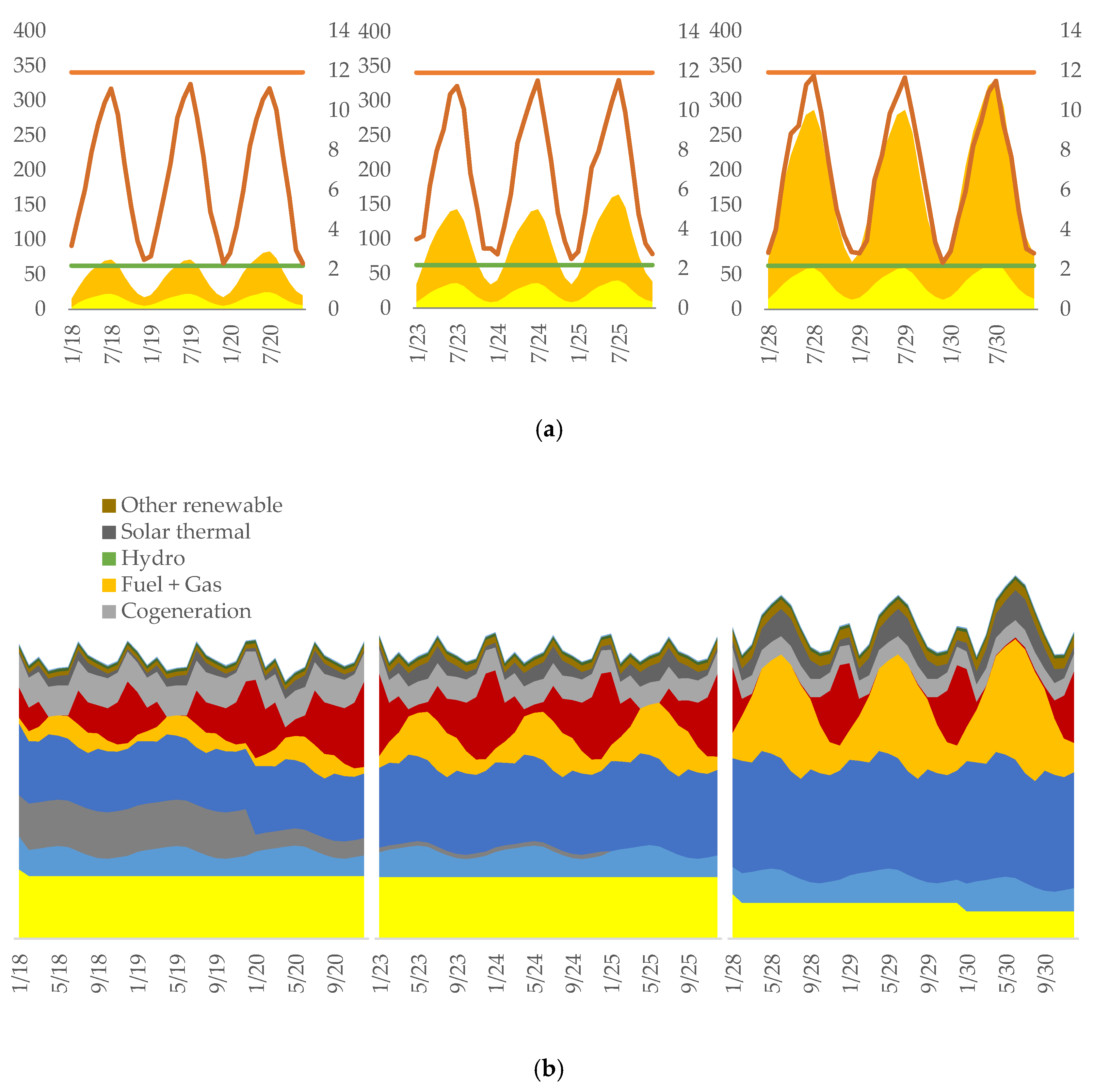
- A progressive substitution of fossil technologies for renewable methods, followed by an evaluation of the behavior of the new model based on a high percentage of these new technologies. Incorporating a low proportion of renewables has not yet caused problems for the security of the electricity supply, but each extra percentage point of renewable energy added exponentially increases the instability of the overall supply.
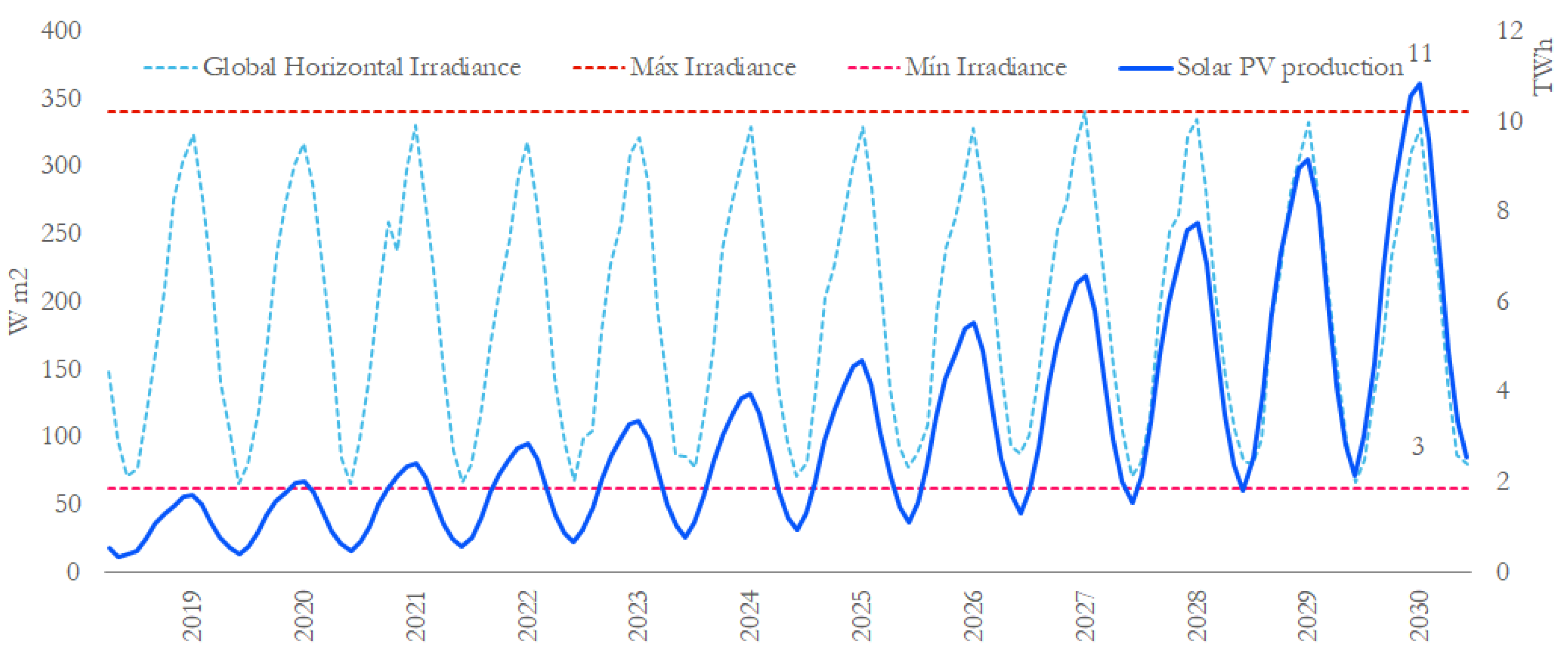
- A robust forecast of electricity demand and solar energy production is highly important. The daily intermittency and seasonality of solar irradiation, at certain times of the year, means that the effort to reach the last of renewable energy could be as important as having reached the first .
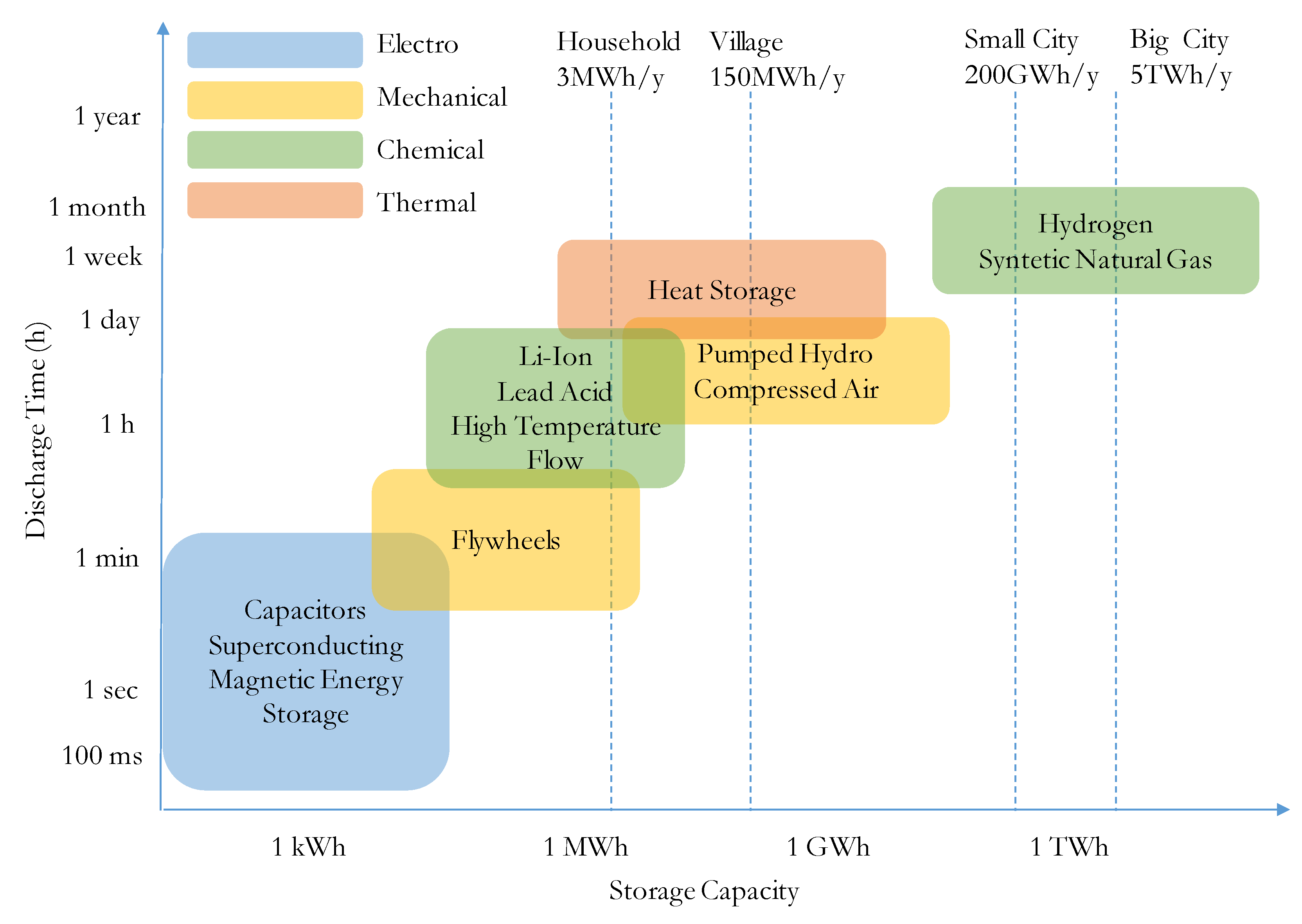
- In such a scenario, energy storage provides flexibility for energy consumption. Until the present decade, electricity has been consumed at the same time it is produced, forcing an effort to synchronize production and demand. Thermal technologies, characterized by their immediacy and high availability, have allowed this model, which now needs to be improved.
Author Contributions
Funding
Conflicts of Interest
Abbreviations
| Mtoe | Million Tonnes of Oil Equivalent |
| R2 | Coefficient of determination |
| PI | Prediction Interval |
| AIC | Akaike information criterion |
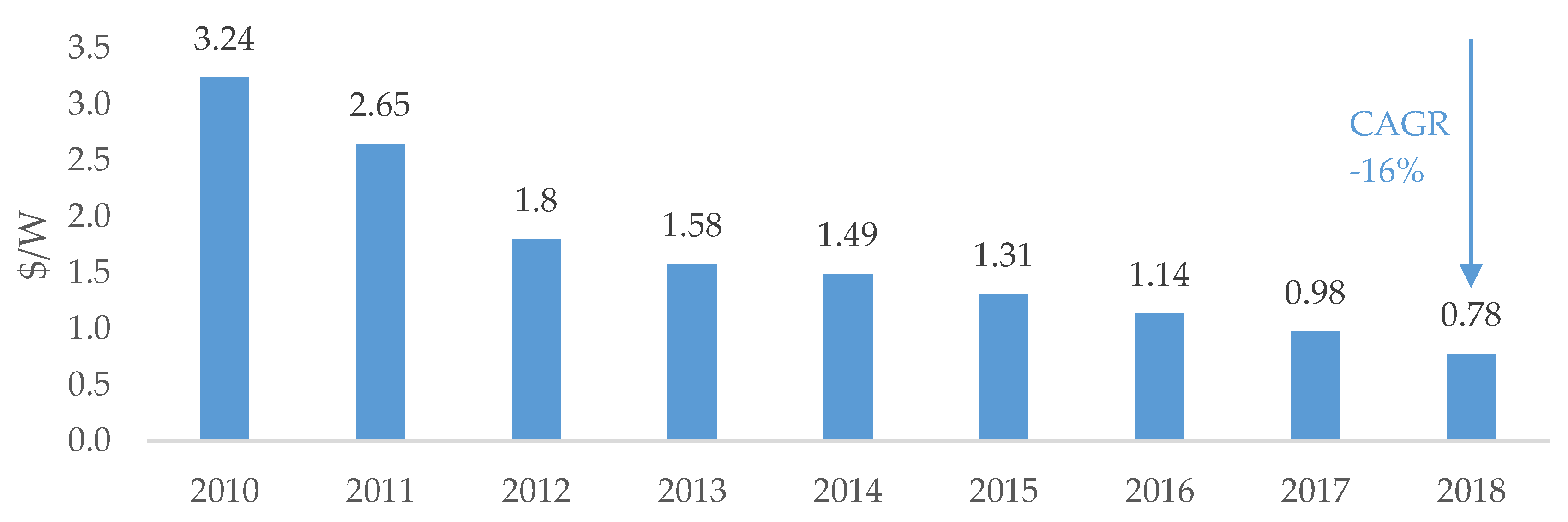
| CAGR | Compound annual growth rate |
| ECEM | European Climatic Energy Mixes |
| C3S | Copernicus Climate Change Service |
| EURO-CORDEX | Coordinated Downscaling Experiment-European Domain |
| LCOE | Levelized cost of energy |
| MAE | Mean absolute error |
| MSE | Mean square error |
References
- Menhat, M.; Yusuf, Y. Factors influencing the choice of performance measures for the oil and gas supply chain—Exploratory study. In Proceedings of the IOP Conference Series: Materials Science and Engineering, Istanbul, Turkey, 8 August 2018; Volume 342, pp. 1–9. [Google Scholar]
- Radoslav, S.D. The Paris Agreement on Climate Change: Behind Closed Doors. Glob. Environ. Politics 2016, 16, 1–11. [Google Scholar] [CrossRef]
- Allam, Z.; Newman, P. Redefining the Smart City: Culture, Metabolism and Governance. Smart Cities 2018, 1, 4–25. [Google Scholar] [CrossRef]
- Hontoria, L.; Rus-Casas, C.; Aguilar, J.D.; Hernandez, J.C. An Improved Method for Obtaining Solar Irradiation Data at Temporal High-Resolution. Sustainability 2019, 11, 5233. [Google Scholar] [CrossRef]
- Qamar Raza, M.; Khosravic, A. A review on artificial intelligence based load demand forecasting techniques for smart grid and buildings. Renew. Sustain. Energy Rev. 2015, 50, 1352–1372. [Google Scholar] [CrossRef]
- Suganthi, L.; Samuel, A.A. Energy models for demand forecasting—A review. Renew. Sustain. Energy Rev. 2012, 16, 1223–1240. [Google Scholar] [CrossRef]
- Alfares, H.K.; Nazeeruddin, M. Electric load forecasting: Literature survey and classification of methods. Int. J. Syst. Sci. 2010, 33, 23–34. [Google Scholar] [CrossRef]
- Hady Soliman, S.A.; Al-Kandari, A.M. Electrical Load Forecasting. In Electrical Load Forecasting; Elsevier: Burlington, MA, USA, 2010. [Google Scholar]
- Almeshaiei, E.; Soltan, H. A methodology for Electric Power Load Forecasting. Alex. Eng. J. 2011, 90, 137–144. [Google Scholar] [CrossRef]
- Yamagata, Y.; Murakami, D.; Seya, H. A comparison of grid-level residential electricity demand scenarios in Japan for 2050. Appl. Energy 2015, 158, 255–262. [Google Scholar] [CrossRef]
- Andersen, F.M.; Larsen, H.V.; Boomsma, T.K. Long-term forecasting of hourly electricity load: Identification of consumption profiles and segmentation of customers. Energy Convers. Manag. 2013, 68, 244–252. [Google Scholar] [CrossRef]
- Pessanha, J.F.M.; Leon, N. Uma metodologia para previsão de longo-prazo do consumo de energia elétrica na classe residencial. II Semin. De Metodol. Do IBGE 2013. [Google Scholar] [CrossRef]
- Bunnoon, P.; Chalermyanont, K.; Limsakul, C. Mid-term load forecasting: Level suitably of wavelet and neural network based on factor selection. Energy Procedia 2012, 14, 438–444. [Google Scholar] [CrossRef][Green Version]
- Shao, Z.; Gao, F.; Zhang, Q.; Yang, S.L. Multivariate statistical and similarity measure based semiparametric modeling of the probability distribution: A novel approach to the case study of mid-long term electricity consumption forecasting in China. Appl. Energy 2015, 156, 502–518. [Google Scholar] [CrossRef]
- De Felice, M.; Alessandri, A.; Catalano, F. Seasonal climate forecasts for medium-term electricity demand forecasting. Appl. Energy 2015, 137, 435–444. [Google Scholar] [CrossRef]
- Wu, J.; Wang, J.; Lu, H.; Dong, Y.; Lu, X. Short term load forecasting technique based on the seasonal exponential adjustment method and the regression model. Energy Convers. Manag. 2013, 70, 1–9. [Google Scholar] [CrossRef]
- Dudek, G. Pattern similarity-based methods for short-term load forecasting—Part 2: Models. Appl. Soft Comput. 2015, 36, 422–441. [Google Scholar] [CrossRef]
- Phuangpornpitak, N.; Prommee, W.; Tia, S.; Phuangpornpitak, W. A Study of Particle Swarm Technique for Renewable Energy Power Systems. In Proceedings of the International Conference on Energy and Sustainable Development: Issues and Strategies (ESD 2010), Chiang Mai, Thailand, 2–4 June 2010; pp. 1–6. [Google Scholar]
- Ünler, A. Improvement of energy demand forecasts using swarm intelligence: The case of Turkey with projections to 2025. Energy Policy 2008, 36, 1937–1944. [Google Scholar] [CrossRef]
- El-Telbany, M.; El-Karmi, F. Short-term forecasting of Jordanian electricity demand using particle swarm optimization. Electr. Power Syst. Res. 2008, 78, 425–433. [Google Scholar] [CrossRef]
- Adhikari, R.; Agrawal, R.K. An Introductory Study on Time Series Modeling and Forecasting Ratnadip; LAP Lambert Academic Publishing: Saarbrücken, Germany, 2013. [Google Scholar]
- Eurostat Regional Yearbook; Publications Office of the European Union: Brussels, Belgium, 2019; ISBN 978-92-76-03505-3.
- Chatfield, C. The Holt-Winters Forecasting Procedure. Appl. Stat. 1978, 27, 264–279. [Google Scholar] [CrossRef]
- Mavromatakis, F.; Franghiadakis, Y.; Vignola, F. Modelling the Power Produced by Photovoltaic Systems. Eng. Technol. Appl. Sci. Res. 2016, 6, 1115–1118. [Google Scholar] [CrossRef]
- Perez, R.; Perez, M. A Fundamental Look at Energy Reserves for the Planet; The International Energy Agency SHC Programme Solar Update: Paris, France, 2015; pp. 4–6. [Google Scholar]
- Lynn, P.A. Electricity from Sunlight: An Introduction to Photovoltaics; John Wiley & Sons, Ltd.: Hoboken, NJ, USA, 2010. [Google Scholar]
- Nemet, G.F. Beyond the learning curve: Factors influencing cost reductions in photovoltaics. Energy Policy 2006, 34, 3218–3232. [Google Scholar] [CrossRef]
- Swanson, R.M. A vision for crystalline silicon photovoltaics. Prog. Photovolt. 2006, 14, 443–453. [Google Scholar] [CrossRef]
- Shockley, W.; Queisser, H.J. Detailed balance limit of efficiency of p-n junction solar cells. J. Appl. Phys. 1961, 32. [Google Scholar] [CrossRef]
- National Renewable Energy Laboratory, NREL. 2018. Available online: www.nrel.gov (accessed on 2 December 2019).
- Schnase, J.L.; Duffy, D.Q.; Tamkin, G.S.; Nadeau, D.; Thompson, J.H.; Grieg, C.M.; McInerney, M.A.; Webster, W.P. MERRA Analytic Services: Meeting the Big Data challenges of climate science through cloud-enabled Climate Analytics-as-a-Service. Comput. Environ. Urban Syst. 2017, 61, 198–211. [Google Scholar] [CrossRef]
- Gelaro, R.; McCarty, W.; Suárez, M.J.; Todling, R.; Molod, A.; Takacs, L.; Randles, C.A.; Darmenov, A.; Bosilovich, M.G.; Reichle, R.; et al. The modern-era retrospective analysis for research and applications, version 2 (MERRA-2). J. Clim. 2017, 30, 5419–5454. [Google Scholar] [CrossRef]
- Troccoli, A.; Goodess, C.; Jones, P.; Penny, L.; Dorling, S.; Harpham, C.; Dubus, L.; Parey, S.; Claudel, S.; Khong, D.H.; et al. Creating a proof-of-concept climate service to assess future renewable energy mixes in Europe: An overview of the C3S ECEM project. Adv. Sci. Res. 2018, 15, 191–205. [Google Scholar] [CrossRef]
- Jacob, D.; Petersen, J.; Eggert, B.; Alias, A.; Christensen, O.B.; Bouwer, L.M.; Braun, A.; Colette, A.; Déqué, M.; Georgievski, G.; et al. EURO-CORDEX: New high-resolution climate change projections for European impact research. Reg. Environ. Chang. 2014, 14, 563–578. [Google Scholar] [CrossRef]
- Astruc, D.; Ruiz, J. Organo-iron mediated synthesis of functional dendrimers with 1 → 3 connectivity. J. Organomet. Chem. 2011, 696, 2864–2869. [Google Scholar] [CrossRef]
- Xue, B.; Geng, J. Dynamic Transverse Correction Method of Middle and Long Term Energy Forecasting Based on Statistic of Forecasting Errors. In Proceedings of the 10th International Power and Energy Conference, IPEC 2012, Ho Chi Minh City, Vietnam, 12–14 December 2012; pp. 253–256. [Google Scholar]
- Fuchs, G.; Lunz, B.; Leuthold, M.; Sauer, D.U. Technology overview on Electricity Storage—Overview on the Potential and on the Deployment Perspectives of Electricity Storage Technologies; ISEA—Institut für Stromrichtertechnik und Elektrische Antriebe, RWTH Aachen: Aachen, Germany, 2012. [Google Scholar] [CrossRef]
- IRENA (International Renewable Energy Agency). Electricity Storage and Renewables: Costs and Markets to 2030; IRENA: Abu Dhabi, UAE, 2017; ISBN 978-92-9260-038-9. [Google Scholar]


| Month | |
|---|---|
| January | |
| February | |
| March | |
| April | |
| May | |
| June | |
| July | |
| August | |
| September | |
| October | |
| November | |
| December | |
| Total |
| Month Number | Month | Demand (GWh) | ||||
|---|---|---|---|---|---|---|
| January | ||||||
| February | ||||||
| March | ||||||
| April | ||||||
| May | () | |||||
| June | ) | |||||
| July | ||||||
| August | ||||||
| September | ||||||
| October | ||||||
| November | ||||||
| December | ||||||
| 253,563 | 12.0 | 254,404 | ||||
| Forecast vs. Demand | 841 | % error | −0.33% |
| Mechanical Energy Storage Systems | Chemical Energy Storage Systems | ||||||||||
|---|---|---|---|---|---|---|---|---|---|---|---|
| Mechanical | Li-Ion | Lead Acid | High Temperature | ||||||||
| Pumped | CAES | Fly-wheel | NMC/LMO | NCA | LiFePo4 | Titanate | Flooded LA | VRLA | NaNiCl | NaS | |
| Energy density (Wh/l) | 0.2–2 | 2–6 | 20–200 | 200–735 | 200–620 | 200–620 | 200–620 | 50–100 | 50–100 | 150–280 | 140–300 |
| Power density (W/l) | 0.1–0.2 | 0.2–0.6 | 5 k–10 k | 100–10 k | 100–10 k | 100–10 k | 100–10 k | 10–700 | 10–700 | 150–270 | 120–260 |
| Lifetime (years) | 30–100 | 20–100 | 15–25 | 5–20 | 5–20 | 5–20 | 10–20 | 3–15 | 3–15 | 8–22 | 10–25 |
| Depth of discharge (%) | 80–100 | 35–50 | 75–90 | 84–100 | 84–100 | 84–100 | 84–100 | 50–60 | 50–60 | 100 | 100 |
| Round-trip efficiency (%) | 70–85 | 40–75 | 70–95 | 81–98 | 81–98 | 81–94 | 81–98 | 75–92 | 75–92 | 80–92 | 70–90 |
| Self-discharge (% per day) | 0.02–0 | 0–1 | 20–00 | 0.09–0.36 | 0.09–36 | 0.09–36 | 0.09–0.36 | 0.09–0.4 | 0.09–0.4 | 0.05–15 | 0.05–1 |
| Energy cost ($/kWh) | 5–100 | 2-84 | 1.5k–6 k | 199–840 | 199–840 | 199–840 | 472–1260 | 105–475 | 105–472 | 315–488 | 262–735 |
© 2019 by the authors. Licensee MDPI, Basel, Switzerland. This article is an open access article distributed under the terms and conditions of the Creative Commons Attribution (CC BY) license (http://creativecommons.org/licenses/by/4.0/).
Share and Cite
Sánchez-Durán, R.; Barbancho, J.; Luque, J. Solar Energy Production for a Decarbonization Scenario in Spain. Sustainability 2019, 11, 7112. https://doi.org/10.3390/su11247112
Sánchez-Durán R, Barbancho J, Luque J. Solar Energy Production for a Decarbonization Scenario in Spain. Sustainability. 2019; 11(24):7112. https://doi.org/10.3390/su11247112
Chicago/Turabian StyleSánchez-Durán, Rafael, Julio Barbancho, and Joaquín Luque. 2019. "Solar Energy Production for a Decarbonization Scenario in Spain" Sustainability 11, no. 24: 7112. https://doi.org/10.3390/su11247112
APA StyleSánchez-Durán, R., Barbancho, J., & Luque, J. (2019). Solar Energy Production for a Decarbonization Scenario in Spain. Sustainability, 11(24), 7112. https://doi.org/10.3390/su11247112