1. Introduction
Presently there is a global problem of energy supply due to several factors. On the one hand, the scarcity of fossil resources hinders the supply of the power demanded. On the other hand, the environmental impact of greenhouse gas emissions imposes constraints on the use of such technologies [
1]. All this implies a high price that is also an obstacle to meet energy needs [
2].
The solutions to this problem have been explored for years in various areas. Among them, the development and integration of generators based on renewable resources (RRs) [
3] is one of the most promising strategies. These types of generators have some drawbacks, mainly related to their cost and the uncertainty of the generation, but they present a sustainable alternative for the development of electricity grids or the reinforcement of existing networks [
4]. Due to the high costs of these systems, feasibility studies to make optimized pre-designs are mandatory. In addition, due to the fact that renewable generation is more fluctuating, these studies are harder compared to the traditional methods based on fixed demand and generation values. If these effects are not taken into account during the design stage, then the investment plans obtained could be inadequate. The sustainable development of electrical power systems by installing and integrating renewable generators also improves the diversity of energy supply and enables the objectives for addressing climate change approved by most countries to be met [
5]. However, despite the aforementioned variable and unpredictable availability of these resources, the methods used to optimize the design of the generation of a network are generally not prepared to be effective and accurate under these conditions [
6].
The optimal design of a power grid is a problem of great complexity that involves combining the appropriate selection of topology with the optimal location, size, and operating strategy of generators. Each of these objectives constitutes a complex problem. The optimal design of the generation system in a power grid (location and size of generators) is a non-linear optimization problem that has received considerable attention in recent years. It can be considered a problem with an economic objective (to minimize the cost of generation), like in [
7], or as a multi-objective problem, if other criteria are added, such as optimizing voltages in buses or reducing CO
2 emissions, for example [
8]. The combinatorial nature of the problem and the mathematical difficulty involved in its solution has often led to evolutionary optimization algorithms, such as particle swarm optimization (PSO), like in [
9], or heuristics (genetic algorithms, for example), like in [
10,
11,
12].
The literature contains many methods for the optimal sizing and placement of generation units in electrical networks, taking into account peak demand and generation values. For example, [
13] showed a problem of optimal placement and optimal sizing of distributed generation (DG) in standard networks. The algorithm used for this purpose was PSO. A very similar example can be found in [
9]. Like in most research works published in this field, these studies used typical peak values for demand and generation and minimized system losses or costs. Sometimes they also analyzed the improvement in the voltage levels in the network [
7], although the method is not designed for that purpose. Other studies have tried to solve the problem using genetic algorithms (GA) [
14]. An example that should be highlighted is [
15], which is a research work with a comprehensive review of evolutionary methods applied to the optimization of DG. In other works, such as [
14] or [
16], the optimization of generator placement using GA and fuzzy programming algorithms was explored. In some studies, demand and generation profiles were used in the design process, as in [
17], where the installation of a plant in a radial distribution network was optimized, using the same demand profile in all the loads of the network.
This kind of study, based on fixed values for demand and generation, may be fine as an approximation to obtain preliminary solutions, and most research works point in that direction. For example, [
18] showed strategies in order to integrate renewable DG and minimize losses. However, these solutions are not optimal in a real situation, where unmanageable generation curves should be considered for each generator. This is especially important for generators based on RRs, such as photovoltaic solar plants or wind farms, since they have great variability [
19]. The availability of generation at every instant of time should be used to achieve the optimal solution. Similarly, the evolution of demand along the day should also be considered. This approach is much more realistic than others used in literature [
20] and it may provide optimal designs for a network to minimize generation costs over time, considering the variations produced between different moments.
On the one hand, these generation scheduling methods will substantially increase the sustainability of power systems by decreasing their costs and effectively integrate RRs and decreasing greenhouse gas emissions. On the other hand, the difficulty of the problem increases considerably. To the knowledge of the authors, no studies have been developed to solve the generation location and sizing problems at once, with a single method, taking into account both demand and generation profiles. This novel approach provides a much more precise way to schedule generation systems for networks and microgrids.
This article proposes a method based on the use of PSO to optimize the different scenarios obtained when considering generation and demand profiles. The convergence of this metaheuristic in complex problems with large networks may be slow or inadequate for predesigns and feasibility studies. To try to accelerate convergence in complex cases, the initialization of PSO population by using the cross entropy (CE) method is explored. An example of the use of CE in optimization problems of electric power systems can be found in [
21]. Additionally, in the present work, the authors explore a hybrid CE-PSO method for complex, time-consuming problems, where CE is used to provide a guided initialization of the set of particles to run PSO. This analysis is a good starting point for future research. The main contributions of this research work are:
The proposed method solves the optimization problems of generation location and sizing in a network simultaneously with a single algorithm;
The method produces a significant improvement in the design of the generation mix in a network, thanks to the use of demand and generation profiles in the design process;
This work compares the designs obtained with demand and generation profiles with those that result in fixed values of these variables, highlighting the improvements produced by the proposed method;
In addition, some results for the improvement of the convergence of the PSO algorithm in cases of high computational cost through a CE-guided initialization are presented.
To illustrate the proposed methodology, two standard Institute of Electrical and Electronics Engineers (IEEE) networks have been adapted. In these networks, realistic demand and generation profiles, obtained through measurements in real facilities, have been assigned to buses. The IEEE 30-Bus system is selected as a base case to conduct an exhaustive analysis of the method and its results. Then, the IEEE 118-Bus system is used as a more complex case to study the improvement in the convergence of PSO algorithm through the initialization by CE. These networks are typical examples for this kind of studies, like in [
22].
The paper is structured as follows.
Section 2 explains the proposed method and develops the mathematical expressions for its implementation.
Section 3 describes the data used for the different case studies.
Section 4 shows the results of the simulations and their discussion. Finally,
Section 5 shows the conclusions of the study.
2. Materials and Methods
Given a network with buses, the goal was to optimize the location and size of a group of generators to be installed, so that the generation cost is minimized. Without loss of generality and in order to improve the sustainability of the system, generators based on RRs were considered. It could be assumed that the initial network had generators, including the connection of a slack bus that was considered bus 1.
Typical demand curves of active and reactive power were known at each bus in the network and maximum and minimum voltage restrictions were considered. The longitudinal and transversal impedances in all the lines were also known.
The set of generators to be added consisted of
photovoltaic generators with generation profiles
,
wind generators with generation profiles
, and
manageable generators (which make it possible to fully regulate both active and reactive power generation), such as biogas or hydraulic power plants. Therefore, the total number of generators to be installed was
and the total number of decision variables was
. Each pair of decision variables was formed by a first integer one (
) with a value in the set
that represents the bus to which each generator was connected and a second continuous one (
) with a minimum value
of 0 (although they could have a lower bound greater than 0), which represents the maximum active power installed for each generator. Thus, the vector of decision variables was composed as:
For each type of generator, the active and reactive power bounds and their typical availability curves were known. For each generator, in each time interval, a generation cost curve was considered according to:
In Equation (2), the variables and refer to the average active and reactive powers generated, respectively, in each time interval (typically one hour, so the average hourly power and the energy demanded in that hour would be the same). Therefore, is the cost (€) of energy production in each interval. The coefficients α and β define the costs based on the type of generator.
In addition, each new generator to be installed was assigned an amortization cost for each day of . This cost was calculated based on the maximum power that the generator delivered among all the intervals, since it was proportional to the minimum necessary size of each generating plant. Therefore, in this calculation, both active and reactive power generation must be taken into account. For existing generators, amortization could also be considered if the cost and age of each generator was known.
The algorithm should define the bus to which each generator in the set of generators should be connected and the active power to be installed without exceeding its upper bound .
Given a certain vector of decision variables
, the network data and the generation curves of each generator were known. Therefore, the optimal power flow (OPF) could be solved by any of the existing algorithms. For this work, the OPF was solved using the Matpower tool in MATLAB [
23] and the “fmincon” algorithm of the Matlab Optimization Toolbox, which is designed to find the minimum of non-linear multivariable functions using the interior-point method. The fmincon algorithm calculates the Hessian by a dense quasi-Newton approximation. The basic operation of the interior-point algorithm is briefly described below. For a more detailed description of similar methods for OPF resolution, other works can be explored, like [
24,
25,
26]. The research work presented in [
27] can be highlighted as a comprehensive review of OPF studies applied to smart grids and microgrids with different methods.
The final goal of this problem was to minimize the total generation costs during a typical day. The day was divided into 24 hours. For a typical day, the hourly demand curve of each bus followed a pattern defined by a curve such as those presented in
Section 3. Similarly, the generation profiles of photovoltaic or wind generators also follow patterns such as those defined in the same section. If several hours had the same demand and generation data, then they could be grouped in a single scenario
, which allowed the consideration of a total number of scenarios
during the day. Consequently, each scenario
took place during
hours.
In view of the foregoing, for each vector
, considering typical profiles for each consumer and for each generator in the network, such as those proposed in
Section 3, the OPF problems in the different scenarios could be solved using the interior-point algorithm. Therefore, the powers
and
generated in each generator
could be obtained for each scenario
. Then, the total generation cost could be computed. Finally, the formulation of the OPF problem
was:
where
, subject to the following equality constraints
:
and subject to the following inequality constraints
:
In these equations, is the generation cost of generator in scenario ; is the rated power of generator (which is known for all existing generators in the original network); subscripts and refer to powers demanded and generated, respectively; is the voltage of bus in scenario . The values of and represent the conductance and susceptance, respectively, in the line that connects two buses, and the angle is the phase between voltage phasors and . In the inequality constraints and are the minimum and maximum voltage limits for bus , respectively; similarly, and are the minimum and maximum limits of active power generated by generator , respectively and and are the minimum and maximum reactive power limits.
After expressing all inequality constraints as upper bound constraints (changing the sign of lower bound constraints), there were
inequality constraints that were converted into equality constraints using a barrier function and a vector of positive slack variables
. Thus, the problem was modified as follows:
subject to:
The parameter of perturbation
must be approaching 0 to solve the original problem. Then, for each value of this parameter, the Lagrangian for the equality constrained problem was as follows:
A feasible interior-point was selected. Then, the partial derivatives and the Hessian of the Lagrangian with respect to were computed and the problem was solved using a quasi-Newton iterative method by updating the perturbation parameter so that it converged to zero.
As a result of the OPF, the active power
and reactive power
generated by each generator in the network that minimize the generation costs for that scenario were obtained. This process was repeated for each scenario (typically for every hour). According to the demand values at every bus in each scenario, the total generation cost could be obtained by adding the costs of all the generators in the network (both the original ones and those proposed by the vector
to be added). Finally, the objective function to be optimized was computed using the following equation:
In this equation, is the total generation cost for that typical day in euros with the vector . In that situation, the power to be installed for generator was . Its calculation was performed using the procedure described below.
For each scenario
, the OPF provided the optimum values
and
of generator
. The minimum necessary power to be installed for that generator was obtained by means of the following equation:
In this equation, is the typical utilization coefficient of generator in scenario , according to its generation curve and is the typical power angle of that generator. Therefore, this calculation corresponded to the minimum power to be installed for generator to be able to supply the necessary active and reactive power according to the OPF result.
Once the minimum cost for the vector was obtained, it was necessary to modify it to cover all possible combinations of its variables. Taking into account the enormous number of possibilities that this represents, the use of the PSO algorithm was proposed to solve the problem of minimizing the global cost . This algorithm is described below.
A sample consisting of particles was chosen. The position of each particle corresponded to a vector . The initial positions of the particles were taken uniformly distributed, trying to cover the entire space of feasible values of every decision variable. In each iteration, each particle obtained a value of the objective function and its best value throughout the algorithm (local best) was stored. In each iteration, the global best value of the objective function so far (global best) was also updated. Typical stop criteria may be the number of iterations or tolerance (small changes in global best).
The steps of PSO algorithm in each iteration were as follows:
Evaluate the value of the objective function of each particle at the current position ;
Update the individual best value of the objective function for every particle (local best) and the global best value of the objective function for the entire population (global best);
Update the velocity of each particle and get its new position for the next iteration.
In each iteration
, the position of every particle
of the sample was updated using the following equation:
where
is the position and
is the velocity of the particle. Velocities must be calculated as:
where
is the particle index,
is the inertial coefficient,
and
are acceleration coefficients (
),
and
are random values (
) regenerated before every velocity update,
is the particle’s velocity at iteration
,
is the particle’s position at iteration
,
is the particle’s individual best solution until iteration
and
is the swarm’s best solution until time iteration
.
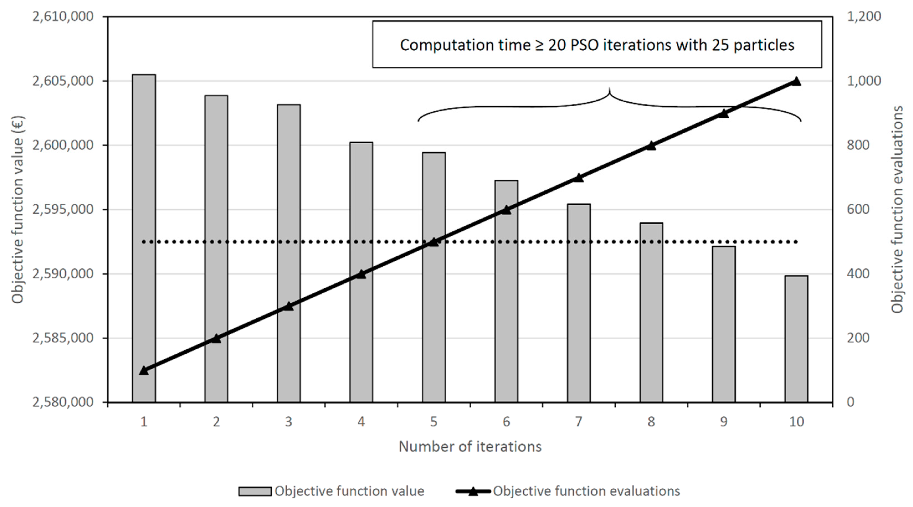
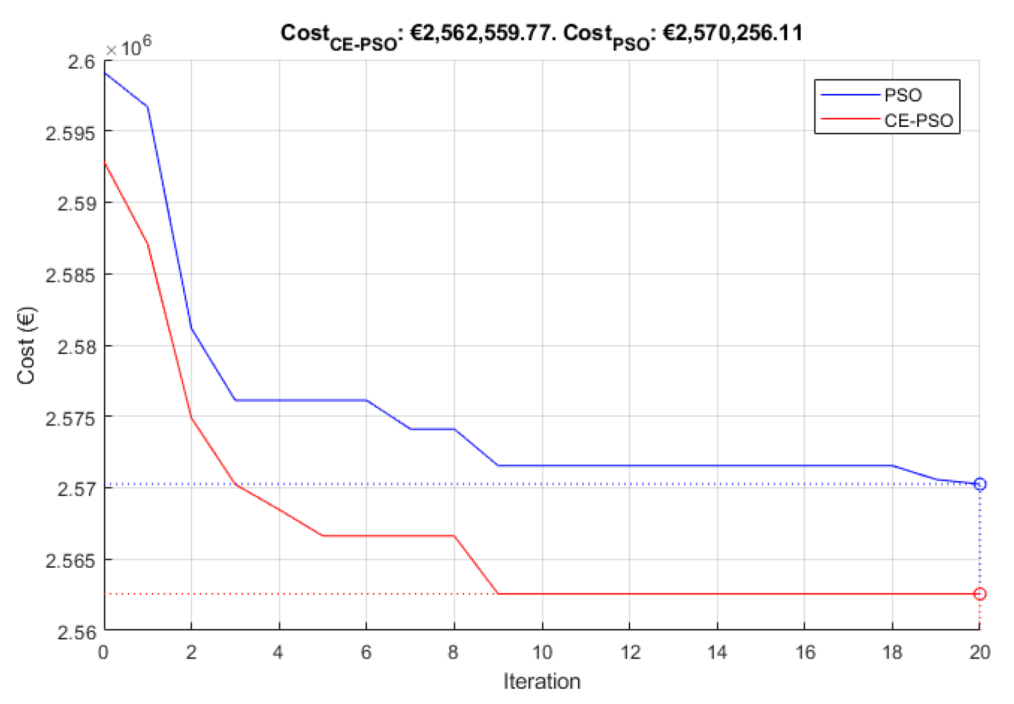
If the network was very large (for example, ), then the computation cost was very high. To make a quick pre-design, the initial population for PSO could be initialized by means of a few iterations of the CE algorithm (for example, four iterations). Four iterations of CE provided a better guided set of particles, which also made it possible to reduce the number of particles for PSO. The second case study was selected to explore this option and some results are included in the results and discussion section.
The CE algorithm used for optimization is described below:
Select an initial sample of uniformly distributed random particles . Each particle represents a vector of decision variables ;
Select the rarity parameter (elitist population ratio) and smoothing parameters and ;
Calculate
and
, mean value and variance of each decision variable in the population using the following expressions:
Initialize the iteration counter ;
Perform an iteration with the following steps:
Compute the objective function of each particle ;
Sort all particles from best to worst;
Select particles as the best fraction of the sorted particles;
Assuming a Gaussian distribution, calculate the distribution parameters for each variable:
Apply smoothing parameters:
Generate a new random sample with a Gaussian distribution using and ;
Finish iteration ;
If , then repeat step 5. Otherwise, end.
For a more detailed explanation of the CE method, other texts can be explored. Among them, [
28] should be highlighted due to the exhaustive explanations and examples that it contains.
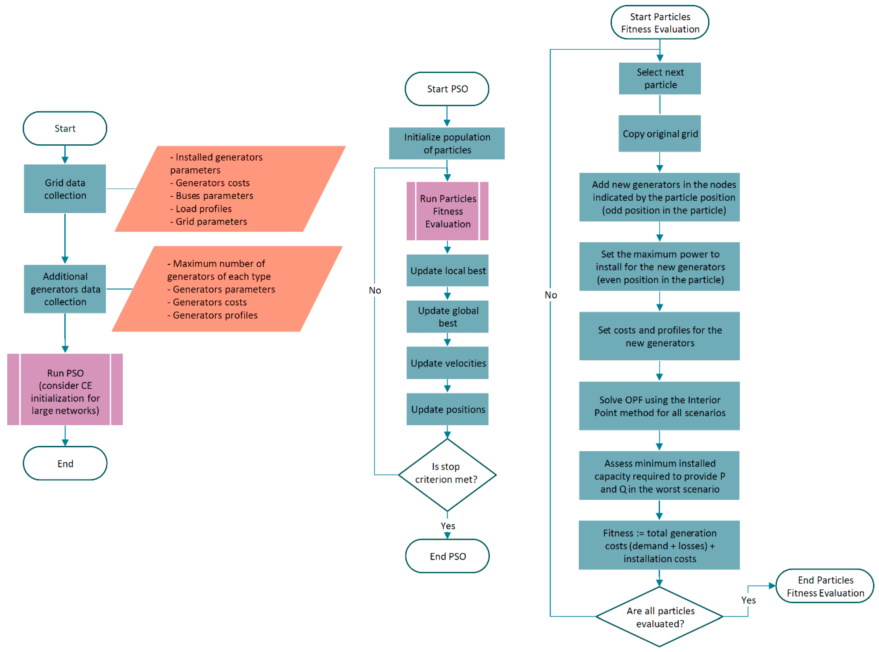
The proposed method, which was called Optimal Generation Scheduling with Dynamic Profiles (OGSDYP), is summarized in
Figure 1.
The main focus of the OGSDYP method is that dynamic profiles should be used to define loads and generators in order to achieve accurate results. The steps to perform a simulation with the method are explained below.
Grid data collection (grid structure and parameters). The typical profiles for every load and every existing generator must be used in the simulation process;
New generators definition. The maximum number of generators of each type to be installed, their maximum size, and their costs must be defined. Generator profiles must be included;
Use PSO to optimize the location (integer variables) and size (continuous variables) of each new generator. This algorithm will provide the nodes and rated power of each new generator. If a generator is not needed, it will be assigned 0 kW;
During PSO, every particle provides a proposal of generation schedule. Then, for every instant of the typical day, the proposed schedule must be optimally managed to determine the minimum cost of every particle. This is performed using interior-point algorithm to calculate every OPF;
By combining generator profile and the power supply scheduled for every hour, the optimal size of every new generator is computed and the objective function value of every PSO particle is calculated;
A new set of particles is generated to continue with PSO algorithm until convergence is reached.
Using the proposed method, some of the drawbacks of the previously published methods in the literature are solved. Thus, the main advantages of the OGSDYP method can be summarized as follows:
The use of a single method (a single simulation) to optimally schedule generation facilities. Most methods use one algorithm to find the optimal types and location for generators and a different one to calculate the optimal sizes [
9]. Others calculate the optimal sizes in a combination of nodes, exploring all possible locations by brute force algorithms [
7]. In the proposed method, if the set of generators is big enough, the OGSDYP method will provide information on which generators to install (how many of each type), in which nodes, and with which size;
The use of dynamic profiles for each generator and each load. Most methods use fixed values, typically average (AVG) or peak values, of active and reactive power in every node [
7,
9,
13]. As the 30-bus system will demonstrate, this may lead to huge differences in total costs in real operating conditions. Other works use curves only for demand facilities or only for generators. Some recent studies use a single demand profile in all nodes in distribution networks [
17]. The proposed method can be applied with different demand profiles of active and reactive power at every node and with different availability profiles for each generator, depending on the type and the geographical location of each power plant. Thus, it is a much more realistic method, with better results, as proven with the case studies. Also, the method may take into account the installation costs of each new generator and the costs of reactive power production, not considered in many previous studies [
20]. Therefore, it includes all advantages of the previous works and provides some new benefits related to accuracy, simplicity, and optimality.
Just as an example to show the complexity of the method and with the purpose of clarifying the usage of every algorithm, let us assume that 25 particles are used in PSO, 20 iterations are performed, and 24 time intervals are considered in the typical day. In this situation, PSO will evaluate the objective function a total of times, and OPF problems will be solved using the interior-point method. Due to this reason, the OGSDYP method involves high computational costs, especially in large networks. This is the reason why the authors highlight the need to develop future research focused on accelerating the convergence of PSO in large networks. Just as an experimental proposal, the authors tested CE initialization in a large network and the results are shown in the second case study. Although the results are not conclusive, this is an interesting starting point for future research.
3. Case Studies
Two standard networks were adapted to test the proposed method. The first one was the IEEE 30-Bus system and the second one was the IEEE 118-Bus system. In each case, the standard network was taken, while maintaining the slack bus generator, to optimize the location and size of the generation to be installed. Some installed generators present in the original network may be considered. However, in the IEEE 30-Bus system, all the previous existing generators were removed, leaving the slack bus as the only initial generator. This ensured that the proposed solution will consist of a set of new generators with high installed powers, which will illustrate the method performance and facilitate the analysis of the results. The slack bus was modeled as a network from which any amount of energy can be imported, but not exported. This was done because if exportation is allowed, then the algorithm can oversize the generators and take advantage of the exportation economically, thus resulting in non-realistic scenarios. The definition of these case studies was made to illustrate the application of the method and the possibilities it offers by analyzing the obtained results. In studies with real networks, the exportation of energy can be considered, taking into account the selling price of energy, as well as adjusting the costs assigned to each generator with real prices for each case. The demand and generation curves obtained to develop these case studies can also be modified. Moreover, specific curves could be assigned to each bus to take into account the geographical position of generators and the influence on their availability.
For each selected network, a classification of the types of consumers in the buses was proposed, taking into account the peak powers demanded in the original case according to the procedure explained below. This procedure was carried out in order to demonstrate the effectiveness of the proposed optimization algorithm for different demand curves in the buses.
The maximum active power demand in the original network was modified using a curve assigned to each bus based on the percentile to which each demand value belonged, according to
Table 1. Thus, the proposed assignment was the result of analyzing the demands of the original network and classifying them into four groups based on their size.
For each type of consumer, the average scaled curve of consumers of that type was used based on actual measurements or real data obtained for this study. Reactive power curves were obtained from the measured active power curves and the typical power factor of the buses where these demand profiles were placed in the original network. Similarly, reactive power limits were considered in generators based on the typical power factor of each type of generator.
The different groups of consumers considered and the assigned curves are described below. The availability curves of solar and wind power plants are also shown according to real data.
3.1. Small Consumer
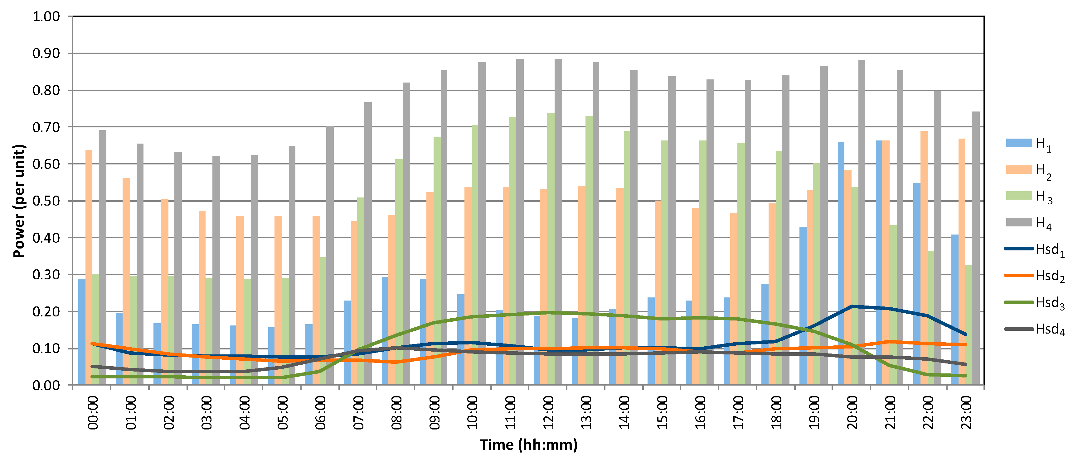
The average hourly active power of a block of 20 homes and a set of five buildings of a university campus used for commercial and service areas was measured for one year.
Figure 2 shows the average curves during the measurement campaign in per unit values
represented with bars and their standard deviation
represented with a line, calculated with Equation (24). This equation considered a sample of
days, where
is the value of the hourly energy of day
at hour
in per unit values (compared to the maximum registered value) and
is the average value for that hour. For this curve, its daily average value
was also obtained, using Equation (25), and its root mean square value
, using Equation (26).
That is, if a bus classified as a small consumer has a maximum registered demand of
in the original network, its average demand at each hour
of the day would be:
3.2. Medium Consumer
The average hourly active power demand of a municipality in Spain with a population of about 500 inhabitants was measured for one year.
Figure 2 shows the average curves during the measurement campaign in per unit values
represented by bars and their standard deviation
represented by a line. For this curve, an average value of
and a root mean square value of
were obtained.
3.3. Large Consumer
The average hourly active power of an administrative, university, and commercial complex with about 90 buildings and a peak power exceeding 16 MW was measured for several years.
Figure 2 shows the average curves for a whole year of the measurement campaign in per unit values
represented with bars and their standard deviation
represented with a line. For this curve, the average value
and the root mean square value
were obtained.
3.4. Very Large Consumer
The demand curves of the Spanish electricity system were obtained for one year from the system operator website [
29]. The average curves during the selected period are shown in
Figure 2 in per unit values
represented by bars and their standard deviation
is represented by a line. For this curve, its average value
and its effective value
were obtained.
3.5. Photovoltaic Generation
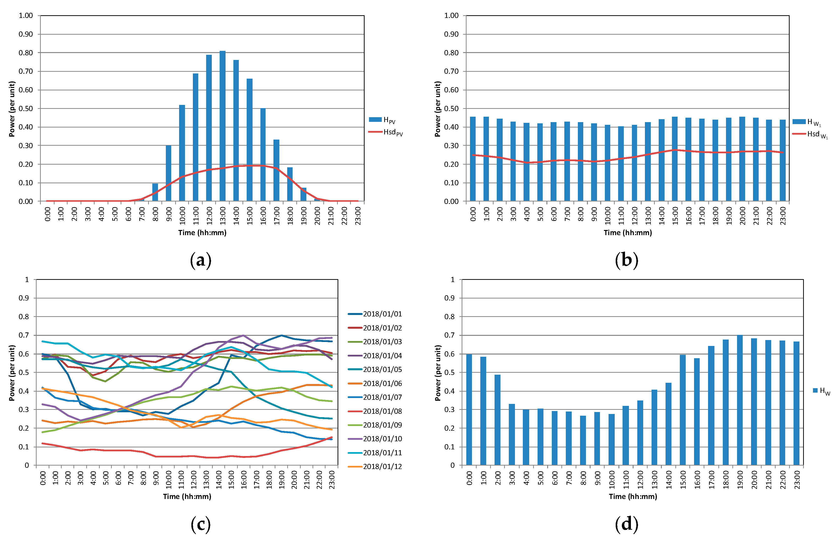
For generation, the curves of the generators to be installed were also analyzed. The average hourly active power generated by a set of 10 photovoltaic solar plants was measured for one year. These plants were approximately located on the latitude line 40°N and the longitude line 1.5°W.
Figure 3a shows the average curves during the measurement campaign in per unit values
represented by bars and their standard deviation
represented by a line. For this curve, an average value of
and a root mean square value of
were obtained. In these generators the power factor will be assumed to be 1.00, so that they cannot provide nor consume reactive power.
3.6. Wind Generation
The average hourly active power generated during one year in the wind power plants of Spain was obtained from the Spanish system operator website [
29]. In
Figure 3b the average curves during the measurement campaign in per unit values
are represented by bars and their standard deviation is represented by a line. For this curve, an average value of
and root mean square value
were obtained. In this type of generator, it was assumed that it is possible to produce reactive power up to a limit of 20% of the installed power.
Figure 3c shows the curves corresponding to 12 consecutive days. Note that this type of resource has a high dispersion and its annual average curve has practically identical values at all hours. Therefore, the use of the average value would not be very realistic nor interesting to illustrate the application of the method. Thus, a random day was selected from among all the available measures to use its curve as
profile of availability for this plant. This profile is represented in
Figure 3d.
3.7. Dispatchable Generators
This group includes plants that can regulate the generation of active and reactive power. Therefore, hydraulic, thermal, or biogas plants, among others, were included here. For this type of manageable generator, an average utilization factor of 90% was considered. It was assumed that they can produce or consume both reactive power and active power with the limit of their installed power reduced by the aforementioned utilization factor.
3.8. Case Study 1
The IEEE 30-Bus system had 30 buses with a total demand of 283.4 MW and 126.2 Mvar. The proposed method was applied after assigning demand profiles, as commented above, and the results are analyzed in
Section 4. Bus 1 was the slack bus and it was considered to be connected to an infinite power grid whose generation was not limited and whose generation costs, according to Equation (1), were calculated with the values
,
,
,
,
.
Active power costs in the slack bus were slightly high to try to reduce the importation of energy and make use of the network’s own generators.
was assigned a small and negative value to represent a higher performance of the generation systems when operating close to the rated power. As for the coefficient
, a value close to the current price of energy exchange in Spain was used [
30]. Reactive power costs were required in order to avoid having generators that only contributed Q when applying the algorithm to solve the OPF. The reactive power cost function was taken as a second-degree monomial to prevent reactive power from providing a benefit when it is negative. As mentioned in
Section 3, in the slack bus, the constraint
must be satisfied.
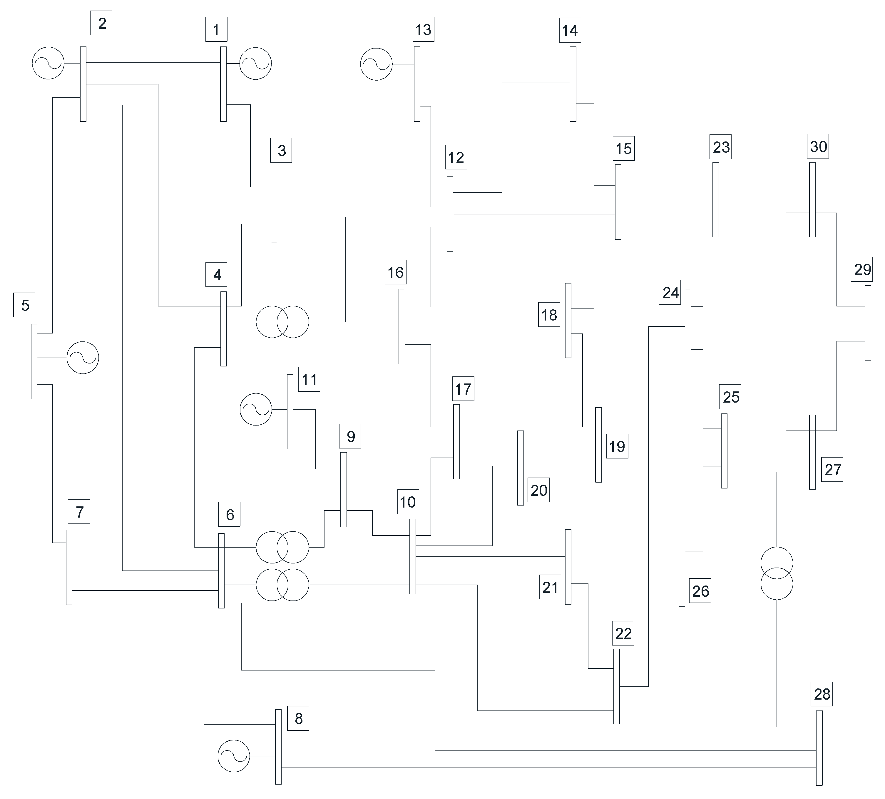
The network diagram can be seen in
Figure 4. The network parameters can be obtained from [
31] and downloaded from [
32].
With the curves assigned as explained, the network demand data are shown in
Table 2.
The optimization of the network design by adding a group of generators according to
Table 3 was proposed for this case study. This group consisted of two photovoltaic generators, two wind generators, and one manageable generator.
The generation costs were calculated with Equation (2) using the values indicated in
Table 3 for each generator. The selected costs were approximate values obtained from real facilities and contrasted with the database available in [
33]. The amortization costs of existing generators (slack) were not considered.
For the calculation of the OPF, a voltage drop limit of ±7% was imposed on all buses, in accordance with current Spanish regulations [
34].
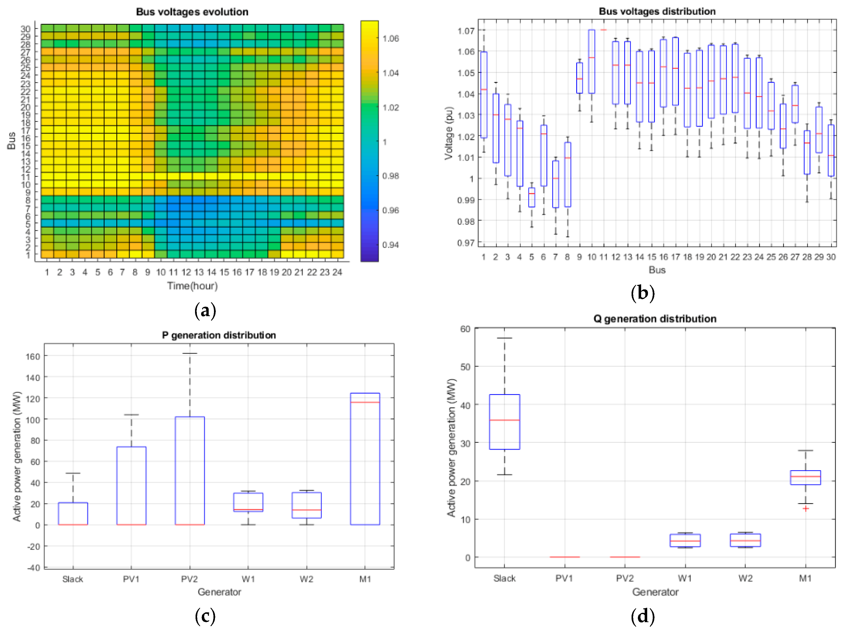
The results of applying the OGSDYP method to the described network are shown in
Section 4. The discussion of these results is also shown in that section.
3.9. Case Study 2
The IEEE 118-Bus System had 118 buses with a total demand of 4242 MW and 1438 Mvar. Without loss of generality, bus 1 was considered the slack bus (bus numbers have been modified) and it was considered connected to an infinite power network whose generation was not limited and whose generation costs were considered as in case study 1.
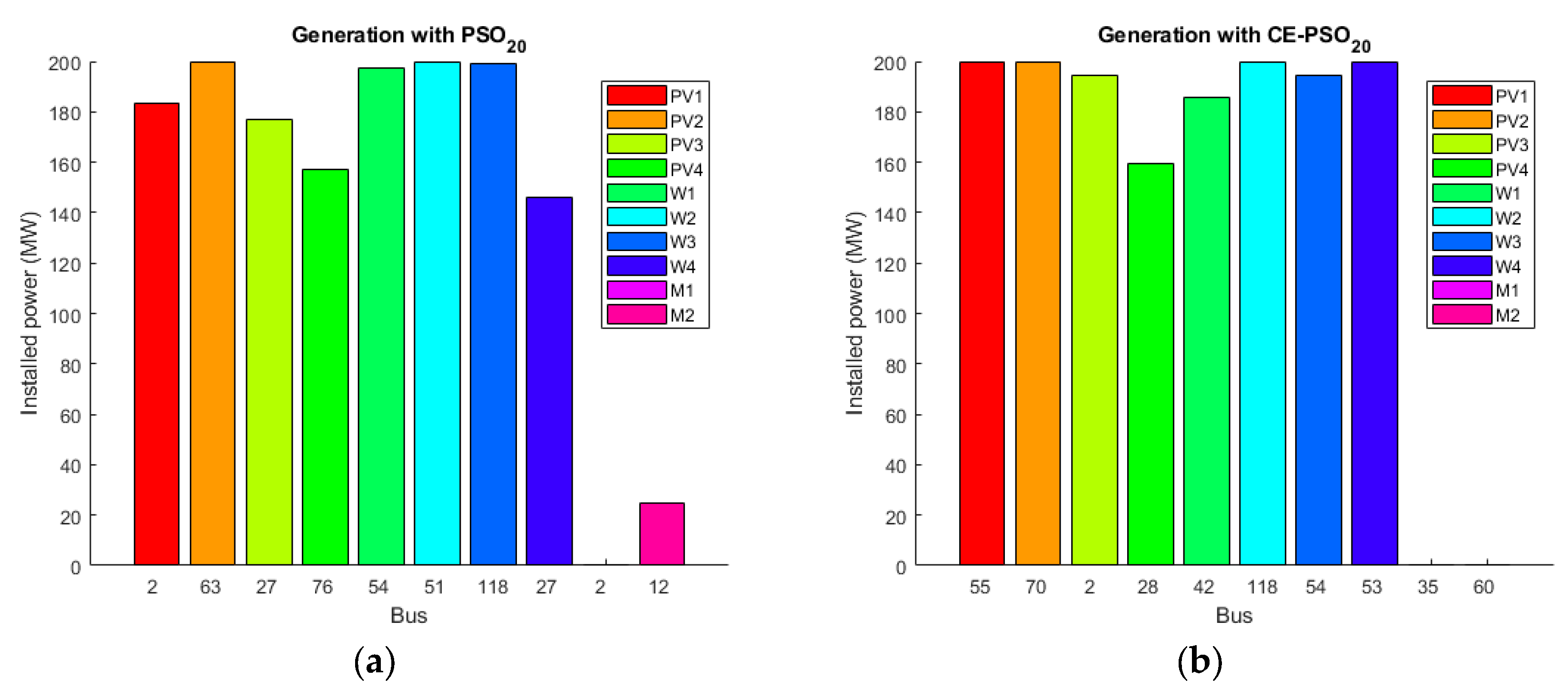
This case study was developed to increase the complexity and analyze the convergence of the OGSDYP method based on PSO. In this case, the 54 existing generators in the network were maintained and 10 generators were added with the same proportion of each type as case study 1. In order to try to improve the convergence of the method, the evolution curve of the randomly initialized PSO was compared using a smart initialization, guided by the CE algorithm. The network data can be found in [
35].
As in case study 1, all consumers were classified in categories
,
,
or
. The proposed generation to add consisted of four photovoltaic, four wind, and two manageable generators with the parameters indicated in
Table 3.
The generators to be added in each network were proposed to include generators of all types with sufficient capacity to provide the total active and reactive power demanded in the network in each scenario. In the resulting generation mix, a significant installed power of RRs was considered, which satisfied the goal of achieving a sustainable development or reinforcement of electricity grids.
The results of applying the proposed method to the described network are shown and discussed in
Section 4.
5. Conclusions
This paper addressed the problem of the optimal location of generators in a power grid, their appropriate size, and operating strategy, to achieve the lowest possible generation costs. The problem was studied by considering dynamic generation and demand profiles to find the optimal global solution.
On the one hand, the economic impact that an inadequate design of the set of generators can have is significant, since it produces an increase in energy prices that could be avoided with a better design. On the other hand, a correct design of the generation systems reduces energy losses and their associated emissions. Moreover, the consideration of renewable power plants in the design process (as is this paper) favors the optimal integration of these energy sources into existing networks. All these objectives contribute to the design of more sustainable networks for the future.
In many countries with unregulated energy markets, the purchase price of energy does not depend on the injection buses of the grid. However, this practice leads to inappropriate designs and higher prices for consumers. The proposed algorithm provides the optimal location and size of new generation facilities in the network. In addition, it is possible to study the effect of a power plant at a specific location. This could be done by including it as an existing generator, and assessing the difference in the generation cost between the original network and a proposed alternative. In power systems, the installation of new power plants in the optimal buses of the network should be enhanced with discounts on energy prices, compared to other buses, where the installation of these power plants can produce a lower benefit in the system operation. This would enhance a better development that could allow a reduction in energy losses (and associated greenhouse gas emissions) and a more sustainable design.
The algorithm presented in this paper was designed to determine the ideal buses for installing new power plants, depending on their type. It also provides the optimum power to install for each of them. Likewise, the algorithm shows the optimal operation strategy of all power plants in the network, both new and existing ones, facilitating the network operation scheduling. To the knowledge of the authors, no algorithm proposed so far has all these features. Taking into account the need to reinforce networks’ generation with RRs to achieve more sustainable scenarios, the cases studied in this work have focused on the installation of renewable power plants (photovoltaic, wind, biogas) in existing networks. Since these types of plants are not manageable in most cases, it was necessary to take into account, in the optimal design, the availability curves of these generators. To optimize the network with dynamic generation profiles, it was also necessary to take into account demand variations. Therefore, the algorithm can be applied with generation and demand profiles that can be entered either individually or by grouping the elements into clusters. In the developed case studies, four types of demand profiles and three types of generation profiles based on real data were used. Nonetheless, individual data could be used for every element, if they were available. This represents an important novelty of this algorithm compared to others proposed in the literature.
Another remarkable feature of the proposed algorithm is that specific costs can be assigned to each generating plant if this information is available. In the case studies, different costs have been assigned according to the type of plant (photovoltaic, wind, biogas), but individualized costs can also be used, since the algorithm queries the cost for each generator during its execution.
The method was tested in detail in a standard network with 30 buses and some simulations were also applied to another standard network with 118 buses. As regards the case studies developed in this work, it should be highlighted that the generation designs made without taking into account the dynamic evolution of demand and generation (for example, using average values) produced results substantially worse than the optimal values. When analyzing these results, significant increases in total generation costs and energy losses were observed. For example, in case study 1, the design of the generation based on average power values in the buses led to a solution whose generation costs were 9.85% higher than the optimal solution obtained with dynamic power profiles. As for the losses, these increased by 103.81% with respect to the optimal case. Additionally, the operation of the grid with designs carried out with fixed values showed lower stability in voltages and a worse usage of resources.
In many literature works, renewable generation is used for DG with small-sized plants, which is applicable to small distribution networks. However, currently, wind farms reach very high power and are usually connected to transmission networks. In addition, the size of photovoltaic power plants is increasing and they are already at powers of hundreds of megawatts, as well as the thermal solar power plants, so these new power plants are also connected to transmission networks. Thus, it is necessary to study the consequences that these plants could have in order to guarantee the optimal operation of these large networks. In this regard, it should be noted that the algorithm can be applied to both small networks (microgrids, distribution networks) and large networks (transmission networks) with the only limitation of the computing costs. This is justified for two reasons. On the one hand, the OPF algorithm used in this work is of general application to any grid. On the other hand, in large networks, the availability curves of plants can be particularized. This means that these curves can be adjusted to the climatic parameters of each location.
Additionally, as a starting point for future research, this paper proposed the use of CE to generate the initial population for PSO for large networks. This strategy seems to lead to better results with fewer iterations, although the results are not conclusive. It may be interesting to study a smart control of a hybrid CE-PSO method in order to reduce the computational cost of these complex problems.
