Article

Spatiotemporal Differences in Determinants of City Shrinkage Based on Semiparametric Geographically Weighted Regression

1
Faculty of Environmental Engineering, The University of Kitakyushu, Kitakyushu 808-0135, Japan
2
Innovation Institute for Sustainable Maritime Architecture Research and Technology, Qingdao University of Technology, Qingdao 266033, China
*
Author to whom correspondence should be addressed.
Sustainability 2019, 11(24), 6891; https://doi.org/10.3390/su11246891
Submission received: 23 October 2019 / Revised: 30 November 2019 / Accepted: 1 December 2019 / Published: 4 December 2019
(This article belongs to the Section Sustainability in Geographic Science)

Abstract

:
City shrinkage, as an ongoing worldwide phenomenon, is an issue for urban planning and regional development. City shrinkage is remarkable in Japan, with over 85% of municipalities experiencing population loss from 2005 to 2015. As Japan’s society ages and with its low fertility rate, city shrinkage has had a tremendous negative effect on economic development and urban planning. Understanding the spatial dependence and spatial heterogeneity of city shrinkage and its determinants is essential for ensuring the sustainable development of a city or region. In this study, a semiparametric geographically weighted regression (SGWR) model was adopted to explore the spatiotemporal differences in determinants of city shrinkage. The results reveal that the SGWR model incorporating the global and local variables is more interpretive compared to ordinary least squares and geographically weighted regression models in exploring the correlates of city shrinkage. We found the spatial dependence and heterogeneity of shrinking cities resulted from demographic, economy, and social factors, and revealed low fertility, the ageing population, and enterprise change ratio influenced city shrinkage in different regions at different times in Japan, whereas foreign population ratio, industry structure, and social welfare had global impacts. The findings provide useful information for understanding city shrinkage at global and local scales.

1. Introduction

As of 2019, more than half of the world’s population is living in urban areas, and the rate is expected to reach 70% by 2050 [1]. Due to rapid urbanization, many environmental effects have become severe and are receiving people’s attention, such as air pollution and urban heat islands. However, city shrinkage, as the antithesis of urbanization, is an ongoing extreme phenomenon not only in developed countries, but also emerging in some fast-urbanizing countries [2,3]. City shrinkage is characterized by population loss, economic downturn, and inefficient land use [4,5,6]. Especially in the developed world, with a background of globalization and de-industrialization, many large cities are considered shrinking cities or will be shrinking cities [7,8,9,10]. Research on the city shrinkage not only provides solutions for the affected regions, but also alerts fast-urbanizing areas about future problems.
The process of city shrinkage occurs within a complex system, so studies on city shrinkage considered many aspects. Many studies focused on the policies and response to city shrinkage and called for local corresponding strategies for the sustainable development of the cities. For example, by assessing four policy responses to city shrinkage in Europe, improving the quality of life of local citizens is the optimal strategy for local government [11]; by identifying the shortcomings of the local government response to city shrinkage as lack of transparency and lack of understanding of best practices, the development of local adaptation policies in shrinking cities is required [12]. Some scholars focused on exploring the factors driving city shrinkage. The driving factors vary from demographics, economy, society, and policies at global and local levels. For example, socio-spatial inequalities were found to more strongly influence city shrinking compared with economic factors in the American Rust Belt [13]; falling birth rates and the effects of German reunification were the main factors affect shrinkage in Germany [14]. The demographic change, which refers to the ageing population and low birth rate, is the primary cause of city shrinkage in Japan [3]; the economic level and population structure are highly related to city shrinkage in China [15]. Although spatial dependence and spatial heterogeneity were confirmed to exist in the city shrinkage spatial distribution [15], previous studies mainly focused on investigating local driving factors of single cities or global driving factors for regions or countries. As studies on policy responses to city shrinkage illustrate the local strategies are more effective and required than corresponding global policies, understanding the local driving factors from the global level is essential for policies makers and actors to better respond to this phenomenon.
Spatial dependence results from various spatial spillover effects, and spatial heterogeneity results from inherent differences between spatial units and variations over space [16,17]. Ordinary least squares (OLS) regression can be used to assess the general correlates of city shrinkage where the correlates are spatially stationary [15]. However, local adaptation strategies are required to identify the spatial heterogeneity of city shrinkage. Geographically weighted regression (GWR) has become an increasingly essential tool for revealing local variables’ effects on the dependent variable over a geographical area [18,19,20,21]. In the GWR model, all the explanatory variables are spatially non-stationary. The semiparametric geographically weighted regression (SGWR) model, which is a mix of OLS and GWR models, is useful in situations where certain explanatory variables influencing the response are global while others are local [22]. Compared with the traditional OLS and GWR models, the SGWR model is usually more interpretive [23,24,25]. As shrinking cities may have several similar characteristics, which are better considered as spatially stationary impact factors, the SGWR model could be more appropriate for modeling the driving factors of city shrinkage.
Following the Meiji restoration, the population of Japan, characterized by urbanization, continued to quickly increase. The population increased from 34 million in 1868 to 128 million in 2008. However, with strict immigration rules, low fertility, and the ageing society, after 2008, the population began to decrease, and many cities became shrinking cities. Compared to other countries experiencing city shrinkage, Japan urban shrinkage is particularly serious. This phenomenon has already significantly influenced the sustainable social development even in large urban agglomerations such as Tokyo and Nagoya [3,26]. Studies on Japan are helpful for understanding the process and mechanism of city shrinkage. As city shrinkage was first proposed to occur due to migration and depopulation [27], population loss is the most indicative phenomenon of a shrinking city [28]. The population change ratio is the most often used indicator to represent the degree of city shrinkage [15,28,29,30,31].
In this study, the population change ratio derived from national census data in 2005, 2010, and 2015 was selected as the city shrinkage index, and a total of 1647 municipalities in Japan were selected as study objects. The objectives of this study were to (1) investigate the spatiotemporal distributions and patterns of shrinking cities in Japan; (2) reveal the interrelationship between city shrinkage and demographic, economy, and social indexes on global and local scales; and (3) compare the determinants across different regions. The findings illustrate the local determinants of city shrinkage in Japan, improve the understanding of the situation and the factors driving city shrinkage, provide valuable information for governments and planners developing effective coping strategies on the global and local levels, and hopefully will draw the attention of fast-developing countries to this possible future issue.

2. Study Area and Method

2.1. Study Area

Japan is a highly developed country, having the world’s third-largest gross domestic product (GDP) [32]. The total population of Japan was about 127 million and the urbanization rate was about 93% according to the National Census in 2015. Japan consists of four main islands, including Hokkaido, Honshu, Shikoku, and Kyushu from north to south, and about 6848 surrounding islands. Japan has 47 prefectures, and each prefecture consists of numerous municipalities, with 1741 in total as of October 2016. Japan is traditionally divided into eight regions, and each region includes several prefectures, excluding Hokkaido (Figure 1). Four types of municipalities exist in Japan: cities, towns, villages, and special wards (the ward in Tokyo). Cities with a certain population are labeled core cities (over 200,000 residents) or designated cities (over 700,000 residents) [31]. In this study, a total of 1647 municipalities on the 4 main islands and surrounding isolated islands were selected as the study items (Okinawa prefecture was excluded). The municipalities were further classified into four categories based on population (Table 1).
Compared with countries such as the United States and China, where the population is growing and city shrinkage is only occurring in local suburban cities or regions [14,29], the city shrinkage situation in Japan is more severe and requires investigation. However, the population in Japan has declined since 2008, and the rate of decline has continued increasing, which indicates that city shrinkage is becoming an increasingly severe nation problem that urgently requires countermeasures. Targeting Japan will improve the understanding of mechanisms of city shrinkage. According to the National Census data in 2005, 2010, and 2015, 71.9% of municipalities experienced continuous shrinkage, and 13.6% of municipalities experienced temporal shrinkage from 2005 to 2015, while only 14.5% municipalities had a continuously increasing population during the period. Specifically, city shrinkage was occurring at a higher rate in towns or villages (80.8%) and small cities (70.4%). However, city shrinkage is not only a phenomenon experienced by local or small municipalities, but 56 large–medium cities were also facing population loss in Japan, indicating an extreme city shrinkage situation in Japan (Table 2). Regionally, the city shrinkage was extreme in Shikoku, Hokkaido, Tohoku, and Chugoku (Table 3). The unbalanced regional economic scale and urban development degree could be essential factors affecting population mobility, which in turn accelerate the ageing population and low fertility in small municipalities.

2.2. Data

We first focused on the spatiotemporal distributions of shrinking cities in Japan. As population loss is the main characteristic of city shrinkage, as the dependent variable, we used the population change ratio from 2005 to 2010, and 2010 to 2015, derived from National Census data downloaded from the portal site of the Official Statistics of Japan.
The age structure, economy level, and social development level were found to be vitally essential issues for urban regeneration, which are directly connected with urban shrinking. Multiple commonly used demographic, economic, and social indicators were selected as the explanatory variables for analysis (Table 4) [15,33,34]. The data were downloaded and derived from Statistical Observations of Municipalities from 2006 to 2016. The explanatory variables consisted of 15 variables from 3 urban sub-systems. In the demographic sub-systems, TP refers to the size of a municipality; UPR, APR, and FPR refer to the age and population structure; in the economic sub-systems, CT and GR refer to the income of local resident and local government, respectively; ECR refers to the industry changes; STIER and STIWR refer to the local industry structure; UR refers to local poverty; in the social sub-systems, SN refers to the local education resources; HN and DN refer to the local medical level; and NEF and NNC refer to the local social welfare level, respectively.

2.3. Methods

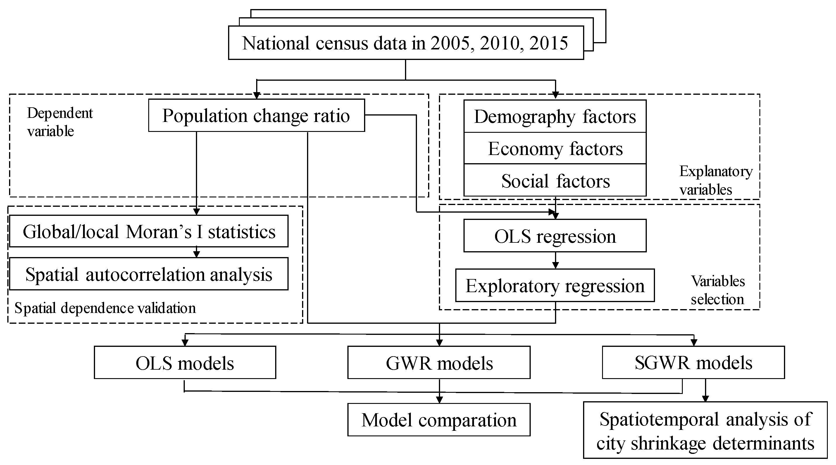
In this study, we first conducted spatial autocorrelation analysis to validate the spatial dependence of population change. Then, OLS and exploratory regressions were employed to identify correlates of city shrinkage. After that, three types of regression analyses, including OLS, GWR, and SGWR, were conducted to reveal the correlates of city shrinkage (Figure 2).

2.3.1. Spatial Autocorrelation Analysis

As nearby objects are more correlated with each other than distant objects [35], the distribution of shrinking cities is more likely to be concentrated in space. Spatial autocorrelation analysis, including the global Moran’s I statistics and local Moran’s I statistics were performed to reveal the spatial dependence of population change. Global Moran’s I, which is a rational number ranging from −1 to 1 after normalized variance was selected for spatial autocorrelation analysis for its widely used to reveal the global spatial autocorrelation. Global Moran’s I > 0 indicates positive spatial correlation where the larger the value, the stronger the spatial correlation; global Moran’s I < 0 indicates negative spatial correlation, where the smaller the value, the larger the spatial difference; and global Moran’s I = 0 indicates a random space. In this study, a larger absolute value indicates greater spatial agglomeration (positive value) or differentiation (negative value) of population change.
However, the global Moran’s I can only reflect spatial autocorrelation but does not identify the location and type of spatial clusters [36]. The Local Moran’s I can be applied to identify the local differences and similarities among neighboring municipalities. The local indicators of spatial association (LISA) can be determined using local Moran’s I [37]. Generally, four clustering/outlier types are classified using the local Moran’s I including (1) high-high cluster (HH), (2) high-low outlier (HL), (3) low-high outlier (LH), and (4) low-low outlier (LL). HH and LL reflect positive spatial correlation; HL and LH reflect negative spatial correlation. Therefore, both the global and local Moran’s I statistics for analyzing the correlation of population variation between each municipality. In this study, HH refers to an above-average rate of population increase in a local municipality, with the same characteristic found in its neighboring cities. HL refers to an above-average rate of population increase in a local municipality, whereas the population decreases in the neighboring cities. LH refers to a shrinkage in a local municipality with above-average rates of population increases in the neighboring municipalities. LL refers to population shrinkage in a local municipality with its neighboring cities showing the same characteristics.
Meanwhile, the spatial weight matrix can significant affect the results of Moran’s I. We selected the k nearest neighbors weight matrix, which set each municipality will have exactly the specified number of neighbors. As a prefecture in Japan has an average of 36 municipalities, the number of neighbors k was select as 40. We used ArcGIS 10.3 (Esri, Redlands, CA, USA) to generate the spatial weight matrix and calculate the global/local Moran’s I, which demonstrated the spatial relationship between the population change in a municipality and its neighbors in Japan.

2.3.2. Screening Explanatory Variables

After testing the spatial autocorrelation of population change, multivariate OLS regression and exploratory regression were conducted to test the relationship between population change and selected explanatory variables. All the variables were first normalized to ensure the variables were normally distribution or approximated normal distribution. Then, to eliminate the multicollinearity of the data, which could produce a distorted or inaccurate model, the variance inflation factor (VIF) for each explanatory variable was calculated, and the variables with a VIF value over 5 were sequentially excluded from the final model until no more VIF > 5 were found [38]. In this procedure, shown in Table A1 and Table A2 (Appendix A), 8 explanatory variables including TP, CT, GR, STIER, SN, HN, DN, and NEF, which had significant multicollinearity with the population change, were therefore excluded from the final model. Then, exploratory regression was conducted to exclude the non-significant variables of the population change at a 95% confidence level. In this procedure, UR was excluded. The results showed that no local multicollinearity existed among the remaining variables. Therefore, after removing the variables redundancy or non-significance, 6 explanatory variables, including UPR, APR, FPR, ECR, STIWR, and NNC, were screened out for both study periods, which suggests the general correlates of city shrinkage remain unchanged. After screening out the variables, the OLS model was reformulated with the 6 explanatory variables. These variables were then used for the corresponding GWR and SGWR models.

2.3.3. Semiparametric Geographically Weighted Regression

Multivariate OLS regression was developed using ArcGIS 10.3 to identify the relationship between the population change and all the explanatory variables from three systems. The traditional OLS model considers all explanatory variables are global and spatially stationary. An OLS model can be expressed as follows:
y i = β 0 + β j x j + ε i
where β 0 represents the intercept, β j represents the regression coefficient for the explanatory variable x j , and ε i represents the error term.
However, in this study, due to the spatial differences in demographics, economy, and society, the GWR model, which considers spatial heterogeneity, could be a better model for reducing the error caused by spatial non-stationary. The GWR model is an extension of the OLS regression model that has been applied to multidisciplinary studies such as meteorology, sociology, and economics, to effectively reveal the spatial heterogeneity. In a GWR model, spatial heterogeneity is investigated in the model fit where the spatial locations of data are incorporated. A local linear regression model for each feature in the dataset was calibrated using a different weighting of observations [39]. The parameter in this model is a single function that represents the spatial location that is derived by weighting all neighboring observations based on a decreasing function of distance [40]. A GWR model can be expressed as:
y i = β 0 ( u i , v i ) + j = 1 p β j ( u i , v i ) x i j + ε i
where ( u i , v i ) represents the coordinates of location i, β 0 ( u i , v i ) represents the intercept, β j ( u i , v i ) represents the local regression coefficient for the explanatory variable x j at location i, and represents the error term. They are estimated using the local weighted least squares method.
A GWR model assumes all the factors are non-stationary and focuses on the differences in the spatial effect of the variables. However, due to population change in Japan being caused by complex factors, the possibility always exists that several global explanatory variables could contribute to explain the population change in Japan. The semiparametric geographically weighted regression (SGWR) model, which is an extension of traditional GWR model, can be applied to meet the requirements of the model and allow some parameters to be global variables and others to be local [19,23,41]. An SGWR model can be expressed as follows:
y i = k = 1 q β k x k + j = 1 p β j ( u i , v i ) x i j + ε i
where k represents the global variables and j represents the local variables. We applied the SGWR model to investigate the spatial impact factors of population change in Japan, using an adaptive bi-square kernel type to calculate the weight matrix. We used an adaptive rather than a fixed kernel because regression points (the center of each municipalities) were irregularly scattered over the study area, and adaptive kernel allows the dataset to be large enough for each local regression [42].
In a GWR model, the accuracy is profoundly affected by the bandwidth, which refers to the number of nearest neighbors of municipality i. The corrected Akaike information criterion (AICc) method [43,44] and the cross-validation (CV) method are two methods often applied to determine the bandwidth. Compared with the CV method, the AICc method can quickly and effectively solve the problem considering the differences in the degree of freedom of different models. Therefore, in this study, the smallest AICc was selected for the appropriate bandwidth determination [19]. The selection of the optimal SGWR model with the smallest AICc based on an iterative process was processed using GWR 4 software [45].

3. Results and Discussion

3.1. Spatial Autocorrelation Analysis of Population Change Patterns

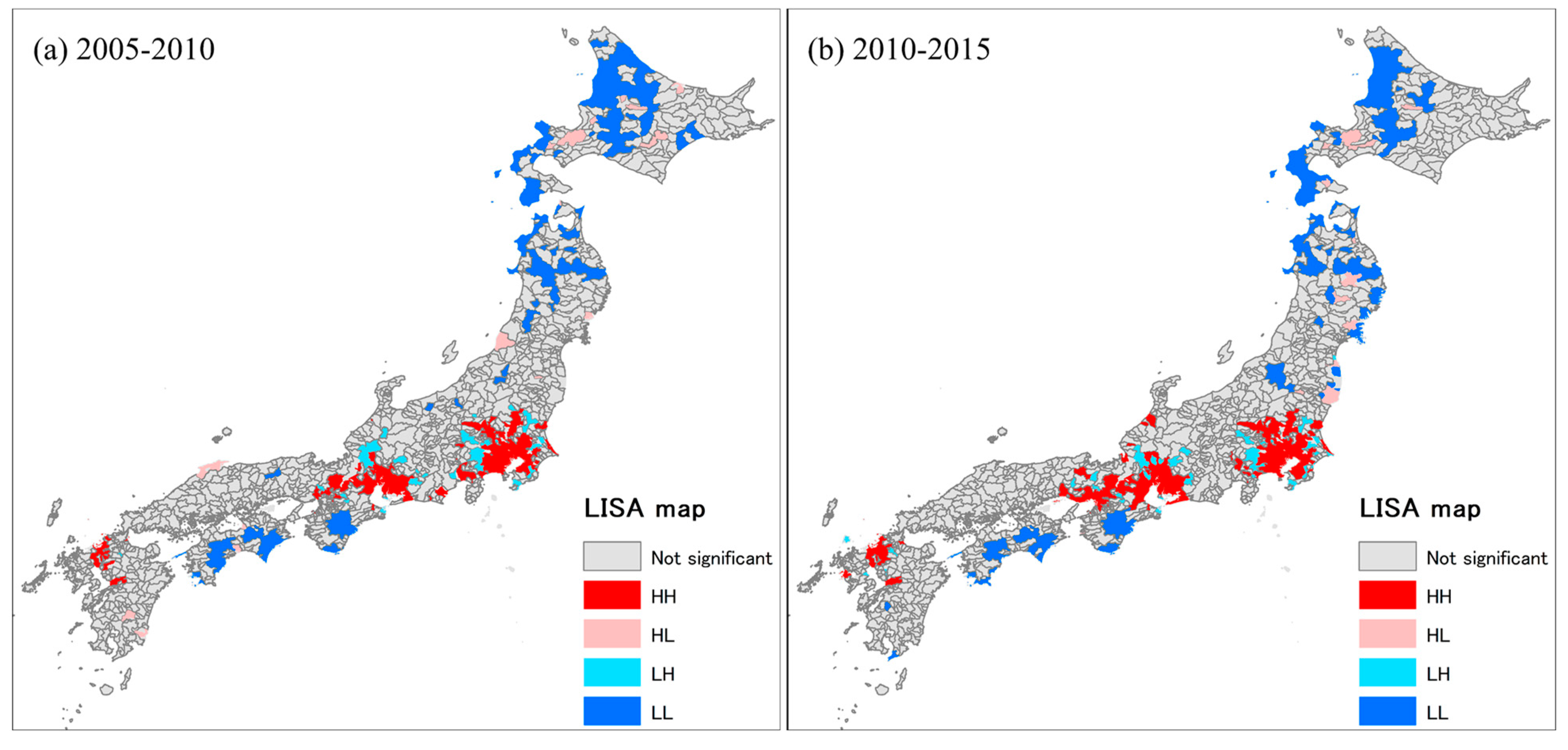
In this study, the population change in Japan from 2005 to 2010, and 2010 to 2015 was confirmed to be positive spatially clustered with the global Moran’s I for the two study periods of 0.462 and 0.615, respectively (Table 5). To further understand the spatial features of population change, local Moran’s I was applied. The LISA maps of population change shown in Figure 3 reveal the local spatial clusters of the population change. During the two study periods, many municipalities showed spatial clustering characteristics. The results show the LL cluster areas were concentrated in Hokkaido, Tohoku, Shikoku, and Kinki, whereas the HH cluster areas concentrated around the Tokyo city cluster in the central area of Kanto, the Osaka city cluster in the southwest of Kinki, Nagoya city cluster in the southwest of Chubu, and the Fukuoka city cluster in the north of Kyushu. Outlier LH areas existed around the Tokyo city cluster and Nagoya city cluster, which indicate that city shrinkage was already occurring in the suburban areas around large urban agglomerations. From 2010 to 2015, the number of cities in the HH and LL clusters increased by 54 and 15, respectively, compared with the period from 2005 to 2010. These results revealed a significant correlation between city shrinkage and spatial distribution and the increasing city shrinkage phenomenon.
Through the global/local Moran’s I statistics, the results indicated the population change patterns were spatially autocorrelated. City clusters centered in Tokyo, Osaka, Nagoya, and Fukuoka demonstrated spatial agglomeration of population growth municipalities, whereas municipalities in Hokkaido, Tohoku, and Shikoku demonstrated the spatial agglomeration of shrinking cities. The unbalanced regional economic scales and urban development degree could be essential factors influencing population mobility, which in turn accelerates the ageing of the population and the low fertility in small municipalities.

3.2. Regression Results

3.2.1. Global and Local Analysis

After screening out the variables, the global model based on the OLS regression procedure was reformulated using the six variables. The results revealed the intercorrelation between population change and municipality parameters, as shown in Table 6.
The results showed that the global model for population change from 2005 to 2010 was moderate (adjusted coefficient of determination (R2) = 0.512), which indicates the six parameters could explain the population change during 2005–2010 to a certain extent. The adjusted R2 of the global model for population change from 2010 to 2015 was 0.715, indicating a substantially adequate explanation of the population change. The results also revealed that APR had a negative coefficient value, which suggests the ageing population ratio has the most significant adverse effect on population change compared with the other parameters. With high positive coefficients, UPR and ECR had significantly positive effects on population change compared with the other parameters. STIWR was found to be non-significant in the first study period, and FPR was found to be non-significant in the second study period. Comparably, the estimated coefficient of UPR increased, indicating an increasing effect of low fertility on city shrinkage. Conversely, the effect of ageing population was found to decrease as the absolute value of APR decreased.
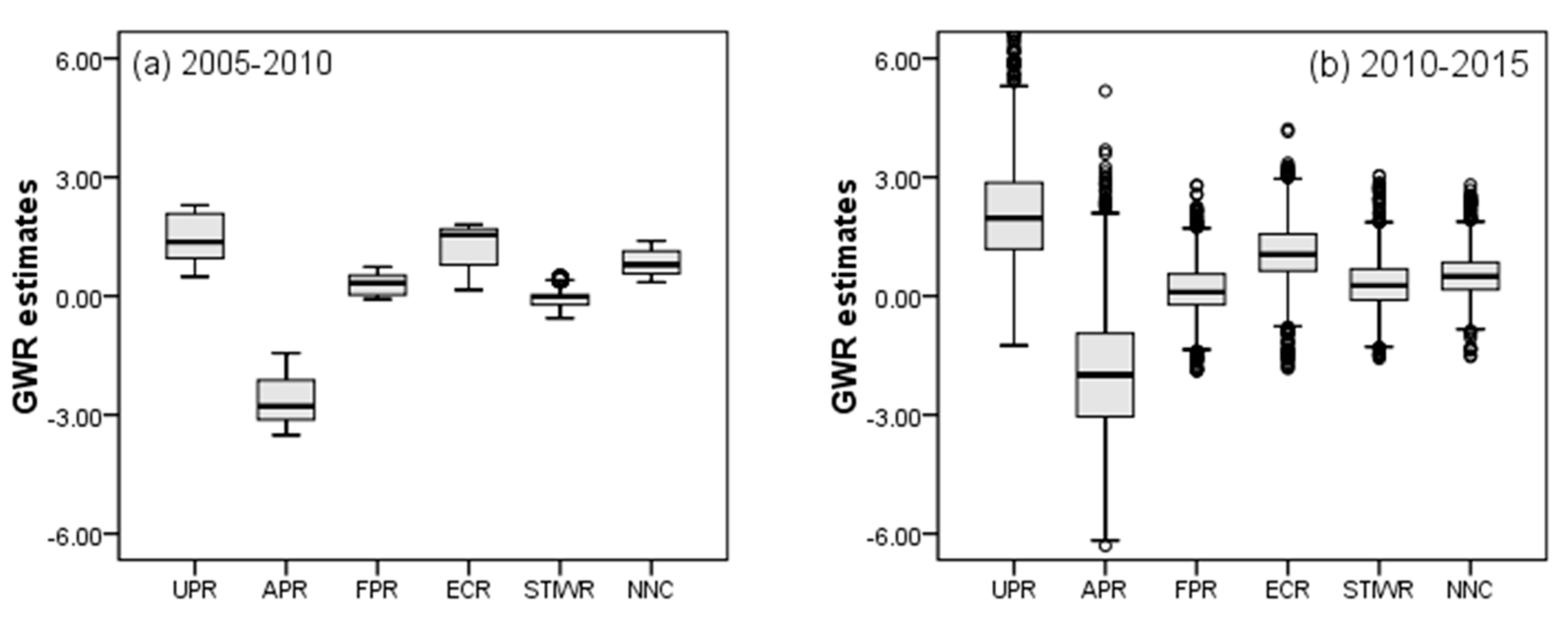
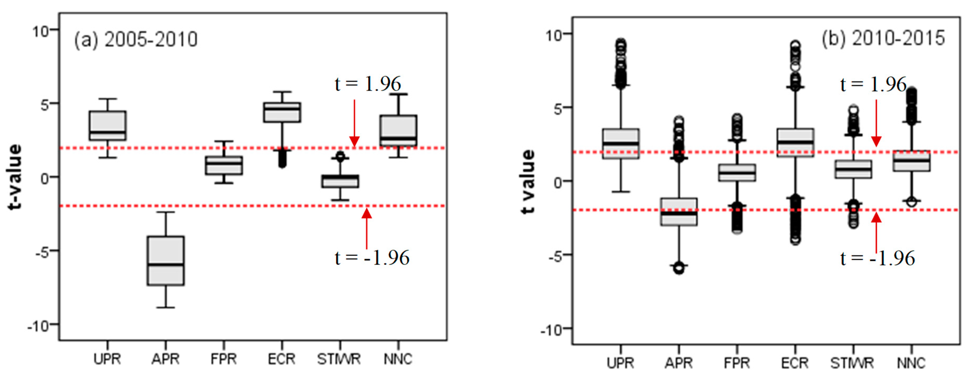
Considering the spatial heterogeneity and spatial autocorrelation of population change, GWR was applied to fit a local population change model. Figure 4 shows the parameter coefficients for the local model of the two study periods. Compared with the first study period, the variation range and the number of mild outliers of the parameters increased. The effects of the parameters could be positive or negative for different regions. Figure 5 shows the variation in parameters’ t-values for the local model. Most observations of UPR, APR, ECR, and NNC reached the 0.05 significance level for the first study period, whereas most observations of UPR, APR, and ECR reached the 0.05 significance level for the second study period.

3.2.2. SGWR Model Analysis

Considering the global model explained the population change to some degree whereas the local model improved the accuracy, the SGWR models were developed to consider both the spatial stationarity and non-stationarity for the parameters affecting population change. An iterative process was used to determine whether a parameter was a global or local variable. The most fitted SGWR model was based on the AICc [43,46]; the model with the smallest AICc value was selected, which refers to the best fitting result. In this procedure, FPR, STIWR, and NNC were selected as global variables, and UPR, APR, and ECR remained local variables for both models (Table 7).
As shown in Table 8, the adjusted R2 for the two local models were 0.528 and 0.815, respectively, which are higher than the global models, suggesting that considering the parameter influences to be spatially non-stationary is more representative than considering them to be spatially stationary. The fitting results of the SGWR model improved compared with the global and local models. The R2 of the SGWR model was the largest compared to the other two models. The AICc value of the SGWR model for the first study period decreased by 47.40, and 10.05 compared with the OLS and GWR models, respectively. For the second study period, the AICc value decreased by 527.43 and 111.89, respectively. Combined with the value of the bandwidth and residual square, we found that the SGWR model was optimal for both study periods, which indicates the population change in Japan displayed spatially stationary and non-stationary parameters.
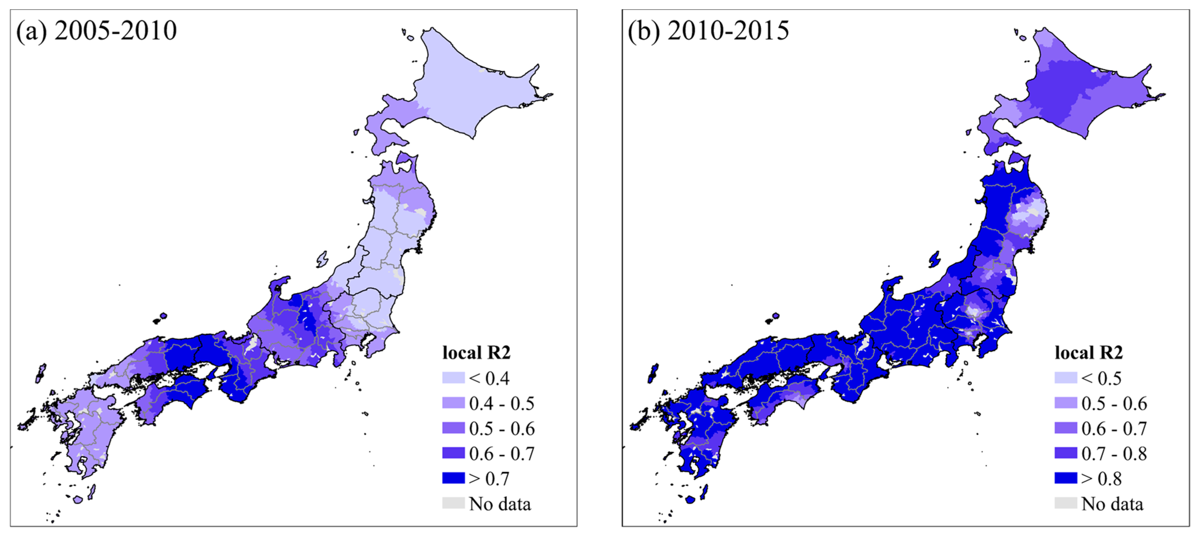
Figure 6 shows the local R2 of the SGWR model. For the first study period from 2005 to 2010, the values of local R2 for Shikoku, Chugoku, Kinki, and Chubu were relatively larger, especially in and around the Osaka city cluster. However, the values of local R2 for Tohoku and Hokkaido were relatively lower, which can be explained by the many municipalities in the two regions experiencing mergers during the first study period. From 1999 to 2010, a wave of merger activity occurred called ‘the great Heisei mergers’ as a response to the low fertility and ageing population. The number of municipalities decreased from 2521 in 2005 to 1727 in 2010. As the merge between municipalities led to a population explosion for those municipalities, the interpretation of the SGWR model for this period was affected, producing a moderate result (adjusted R2 = 0.532). However, since 2010, the municipality mergers ceased and little change occurred in the administration districts from 2010 to 2015, explaining the high value of local R2 in most regions in Japan during this period.
For UPR, APR, and ECR found to be non-stationary spatial correlates affect the population change, the local coefficients of each variable and the spatial characteristics of city shrinkage correlates were analyzed. The t-test was conducted to pick out the coefficients of the local variables which passed the significance level of 0.05.
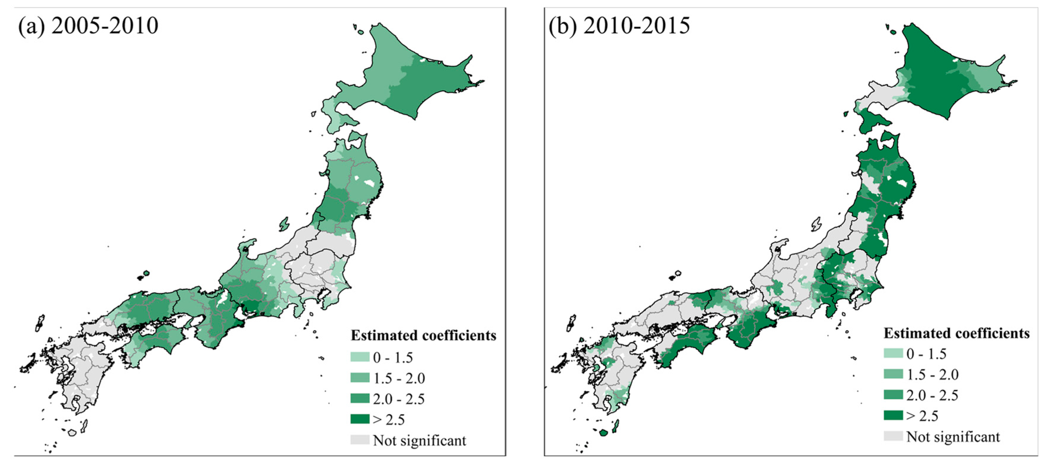
Figure 7 depicts the local coefficients of UPR from 2005 to 2010, and from 2010 to 2015, UPR had a significant positive effect in 1074 and 988 municipalities (p < 0.05) for the two study periods, respectively. The results indicated that from 2005 to 2010, the ratio of the underage population mainly affected the population change around Nagoya city cluster, whereas from 2010 to 2015, the underage-population-affected areas were scattered and extended to south Kinki, east Shikoku, and the boundary area between Chubu and Kanto, and the north and south parts of Kyushu. UPR remained correlated with the population change in most parts of Hokkaido and Tohoku from 2005 to 2015. Different from the other countries facing city shrinkage, even countries in East Europe, city shrinkage is most strongly linked to demographic transition and process of an ultra-ageing society [34,47]. The results indicated that low fertility rate could be the key factor influencing the city shrinkage and the ageing population [48,49]. Since 2007, the fertility rates have continued decreasing and began to fall below death rates. City shrinkage in Hokkaido and Tohoku, where the underage population ratio was below the national average, have always been affected by low fertility rates. As the fertility rate continues to fall, it would become a main factor affecting the city shrinkage in the other regions.
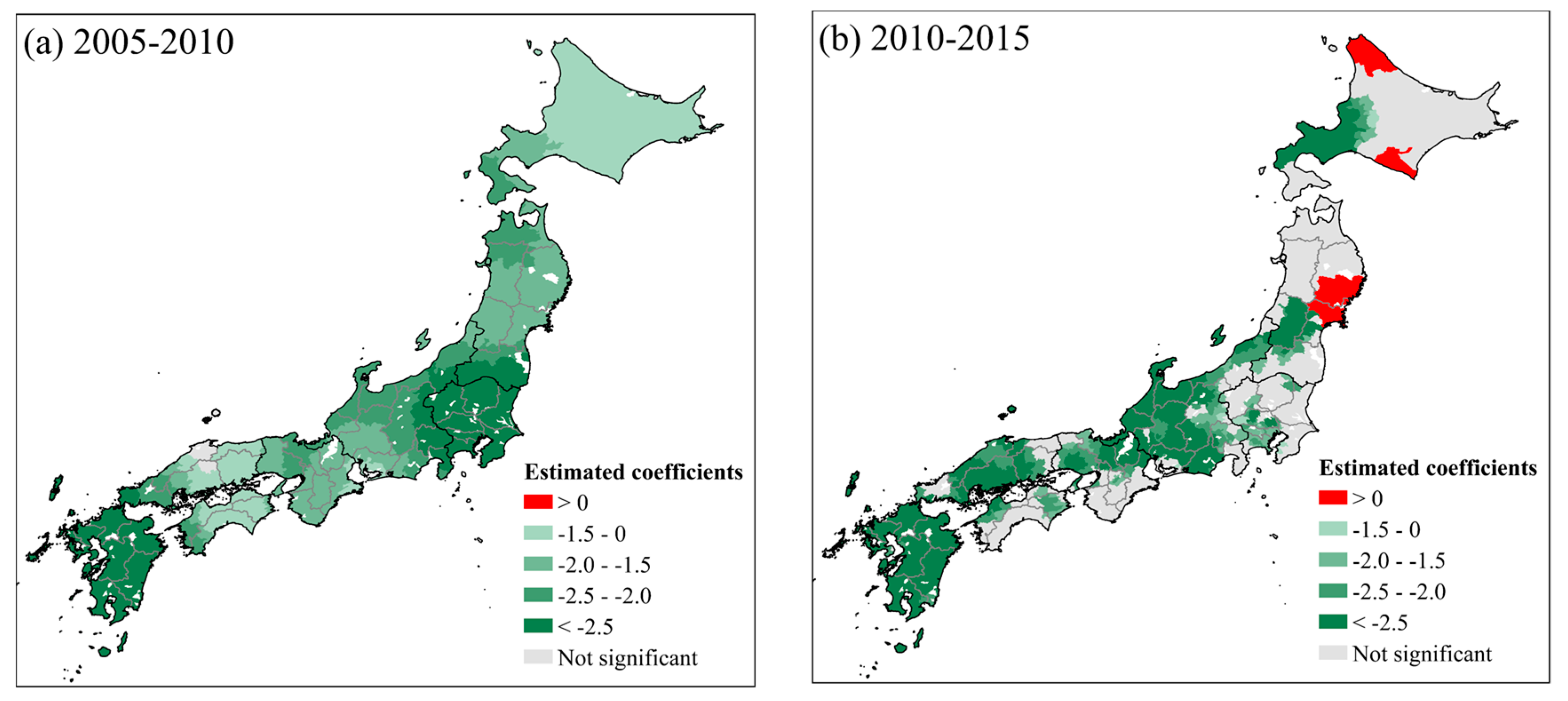
Figure 8 shows the coefficient of the ageing population effect on population change from 2005 to 2010 and from 2010 to 2015. In the first period from 2005 to 2010, only 10 municipalities did not pass the significance test, whereas the other municipalities were found to have a negative correlation between UPR and population change, which suggests the ageing population is correlated with driving city shrinkage nationwide. However, the estimated coefficient of UPR varied between regions. Kyushu and Kanto were the regions with the largest UPR estimated coefficients. The ageing phenomenon in Kyushu was serious, especially in the south, which has aggravated the city’s shrinkage. Conversely, in Kanto, centered in Tokyo, the labor force continuously migrated inward and the proportion of the elderly population continued to decline, which has caused urban expansion in the region. The city shrinkage in the distant periphery and suburban areas occurred due to the ageing populations and infrastructure that has become inadequate [50,51]. From 2010 to 2015, the area of the ageing population effect shrunk and negative coefficients were found in 935 municipalities mainly concentrated in Kyushu, Chubu, and Chugoku. However, positive coefficients were found in 45 municipalities in south Tohoku and south and north Hokkaido, which could be due to the aggregation of the elderly population and population ageing.
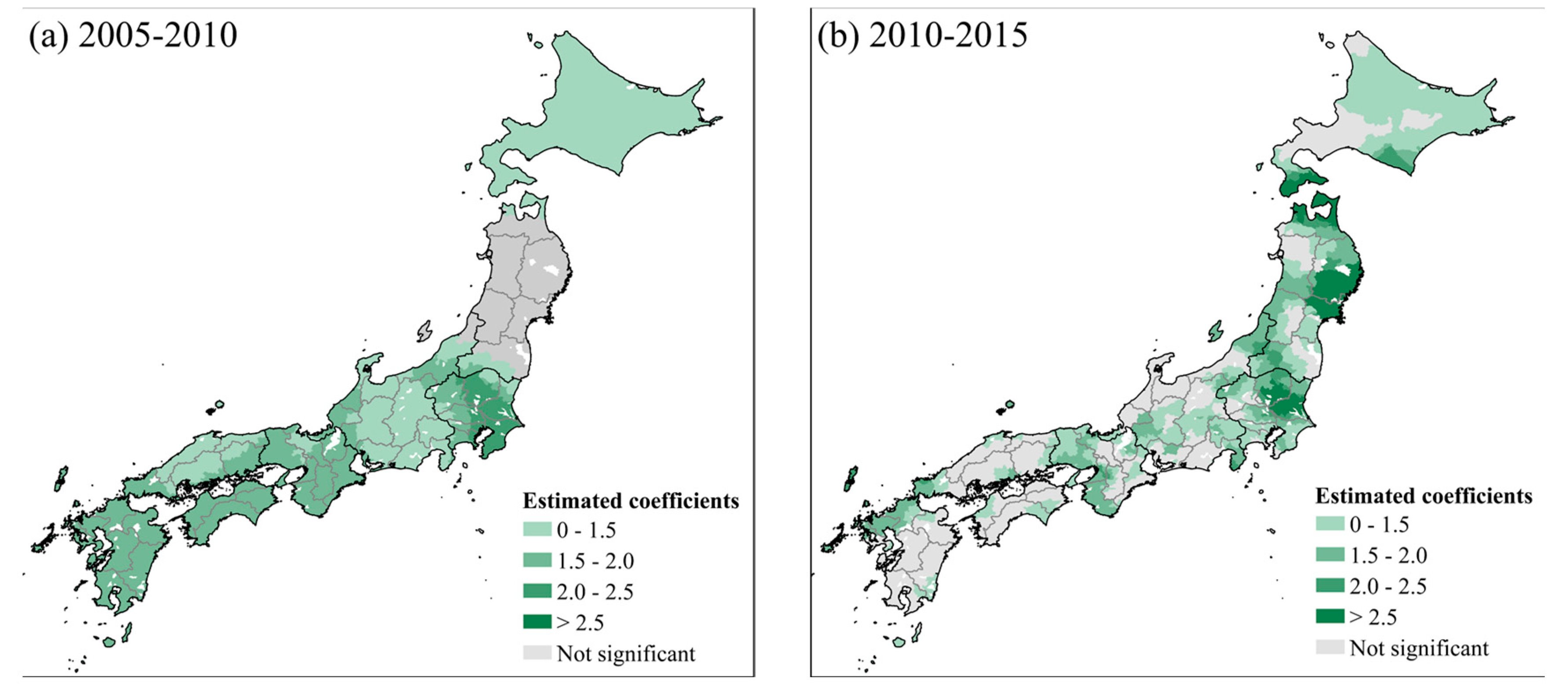
Figure 9 shows the spatial distribution of the local ECR coefficient from 2005 to 2010 and from 2010 to 2015. The local ECR coefficient was found to be spatially non-stationary, and the differences between the two study periods in the region varied. Generally, the economic correlates less impacted city shrinkage than the demographic correlates. From 2005 to 2010, the local ECR coefficient for Kanto was the largest, followed by Kyushu, Shikoku, and Kinki, indicating the population changes in those four regions were strongly correlated with the number of enterprises. However, the non-significant correlation in Tohoku indicated that the population changes in the region were not correlated with the number of enterprises. Comparatively, from 2010 to 2015, the local ECR coefficient for 81.7% of municipalities in Tohoku was significantly positive. The number of enterprises decreased, which was an essential reason for population decline and city shrinkage in the region. The results revealed that the changing numbers of enterprises was significantly correlated with the population change in several main city clusters in Japan, which are also the economic centers, including Tokyo, Osaka, and Fukuoka, for both periods. Urban agglomerations benefit from the increase in the number of enterprises, which appeals to the working population and stimulates population agglomeration and urban expansion [52,53], thus leading to the population loss and city shrinkage in small cities far from metropolises.
Other studies explained city shrinkage in Japan as being due to the ageing population, low fertility, and de-industrialization at a global level [49,54]. However, few studies focused on the quantitative differences of determinates that contribute to city shrinkage. As city shrinkage worldwide refers to the loss of population, it is a severe phenomenon accompanied by economic, social, and cultural decline [55,56]. As the global and local Moran’s I statistics showed spatial aggregation for the population change ratio, we considered the variables to have spatially stationary or non-stationary effects on city shrinkage in Japan, and encouraging us to explore the regional differences in city shrinkage from 2005 to 2015. The results revealed the spatial heterogeneity of shrinking cities, and showed UPR, which refers to low fertility, dominated city shrinkage in Hokkaido, Tohoku, and Kinki; APR, which refers to the ageing population, dominated in Chubu and Kyushu; and ECR had a significantly positive effect in Kanto. In the two study periods, the influence of the local variables in different regions were quite different. Generally, demographic indexes were found to be more correlated with city shrinkage in Japan, which validates that the demographic transition had more of an effect than economic transition. The results showed that APR have the largest absolute value of the estimated coefficients, which indicate ageing population could be a key factor influencing city shrinkage in most municipalities in Japan from 2005 to 2010, whereas low fertility could be the key factor influencing city shrinkage from 2010 to 2015.

4. Conclusions and Prospects

In this study, we developed SGWR models to capture the spatiotemporal differences in determinants affecting city shrinkage in Japan based on national census data from 2005 to 2015. Our findings are as follows: (1) City shrinkage in Japan is a serious national problem, which showed a significant increasing positive spatial autocorrelation; Hokkaido, Tohoku, and Shikoku had the largest shrinking city clusters, and this phenomenon has already occurred in suburban areas around the Tokyo and Nagoya city clusters. (2) Compared with traditional OLS and GWR models, the SGWR models, which consider spatial dependence and heterogeneity, are more interpretive in the explanation of city shrinkage. (3) The correlation between the demographic, economic, and social indexes and city shrinkage was revealed through quantitative analysis. Low fertility, ageing population, and industry changes, expressed by APR, UPR, and ECR, were the critical spatially non-stationary correlates, with large estimated coefficients, affected the city shrinkage in different regions at different times. The findings contribute to improving our understanding of the situation and correlates of city shrinkage, and provide valuable information for governments and planners when developing effective coping strategies for city regeneration.
Due to low fertility and strict immigration policies in Japan [34], which mean city shrinkage may be an irreversible process, determining how to ensure the smart decline of city sizes is an essential issue [57]. The limitation of this study is that specific policies were not considered as an explanatory variable. Future studies are required to analyze the implementation of specific policies and their effect on city shrinkage, and to explore the characteristics of spatial patterns of city shrinkage in each city using more sophisticated data.

Author Contributions

Conceptualization, W.P. and W.G.; formal analysis, W.P. and R.W.; methodology, W.P.; writing—original draft, W.P. and J.J.; writing—review and editing, W.G., X.Y., R.W., and J.J.

Funding

This research received no external funding.

Conflicts of Interest

The authors declare no conflicts of interest.

Appendix A

Table A1. Variance inflation factor (VIF) value of variables selection procedure of the model study period 2005 to 2010.
IterationTPUPRAPRFPRCTGRECRSTIERSTIWRURSNHNDNNEFNNC
1 (keep all)208.95 3.62 4.98 1.28 167.45 33.62 1.25 47.16 2.40 1.84 12.61 25.56 14.10 8.65 4.61
2 (remove CT)52.01 2.98 4.02 1.21 -32.10 1.24 45.64 2.03 1.31 12.44 25.00 13.73 8.29 4.14
3 (remove TP)-2.97 4.01 1.21 -29.75 1.24 30.78 2.02 1.21 12.41 23.99 13.50 8.29 4.09
4 (remove STIER)-2.96 3.91 1.18 -25.10 1.24 -1.78 1.21 12.01 22.84 12.71 7.87 4.08
5 (remove GR)-2.93 3.90 1.18 --1.24 -1.74 1.21 9.10 20.08 12.62 7.66 3.64
6 (remove HN)-2.93 3.77 1.18 --1.21 -1.68 1.20 8.22 -10.08 7.39 3.62
7 (remove DN)-2.91 3.59 1.18 --1.19 -1.51 1.20 6.80 --6.70 3.61
8 (remove SN)-2.88 3.52 1.17 --1.18 -1.49 1.20 ---6.08 3.54
9 (remove NEF)-2.82 3.50 1.16 --1.18 -1.48 1.19 ----1.19
Table A2. Variance inflation factor (VIF) value of variables selection procedure of the model study period 2010 to 2015.
IterationTPUPRAPRFPRCTGRECRSTIERSTIWRURSNHNDNNEFNNC
1 (keep all)211.51 1.51 4.53 1.07 169.83 17.78 2.03 48.41 2.03 1.72 26.22 13.50 15.35 10.24 1.28
2 (remove CT)42.80 1.51 4.46 1.07 -16.12 1.17 42.25 1.81 1.26 11.75 12.78 13.10 9.90 1.28
3 (remove TP)-1.50 4.28 1.07 -15.72 1.15 22.38 1.77 1.16 11.42 11.95 13.02 9.87 1.27
4 (remove STIER)-1.48 4.29 1.07 -15.53 1.14 19.76 1.74 1.16 11.30 11.84 10.13 9.75 1.27
5 (remove GR)-1.44 4.27 1.07 --1.11 -1.64 1.16 10.80 11.11 8.02 9.46 1.26
6 (remove HN)-1.31 4.30 1.07 --1.10 -1.63 1.16 8.82 -7.31 8.84 1.26
7 (remove NEF)-1.28 4.29 1.06 --1.10 -1.62 1.15 7.13 -6.44 -1.25
8 (remove SN)-1.25 4.28 1.06 --1.09 -1.54 1.15 --6.21 -1.25
9 (remove DN)-1.21 4.08 1.06 --1.08 -1.44 1.14 ----1.24

References

  1. UN. 2018 Revision of World Urbanization Prospects; United Nations Department of Economic and Social Affairs: New York, NY, USA, 2018.
  2. Haase, A.; Rink, D.; Grossmann, K.; Bernt, M.; Mykhnenko, V. Conceptualizing urban shrinkage. Environ. Plan. A 2014, 46, 1519–1534. [Google Scholar] [CrossRef] [Green Version]
  3. Mallach, A.; Haase, A.; Hattori, K.J.C. The shrinking city in comparative perspective: Contrasting dynamics and responses to urban shrinkage. Cities 2017, 69, 102–108. [Google Scholar] [CrossRef]
  4. Hattori, K.; Seike, Y.; Yoshida, Z.; Hamaguchi, S.; Yamada, H.; Suzuki, N.; Itami, K.; Kamada, Y.; Inoue, N.; Uchida, T. Shrinkage of tokamak current channel by external ergodization. J. Nucl. Mater. 1984, 121, 368–373. [Google Scholar] [CrossRef]
  5. He, S.Y.; Lee, J.; Zhou, T.; Wu, D.J.C. Shrinking cities and resource-based economy: The economic restructuring in China’s mining cities. Cities 2017, 60, 75–83. [Google Scholar] [CrossRef]
  6. Hospers, G.-J. Coping with shrinkage in Europe’s cities and towns. Urban Des. Int. 2013, 18, 78–89. [Google Scholar] [CrossRef]
  7. Großmann, K.; Bontje, M.; Haase, A.; Mykhnenko, V.J.C. Shrinking cities: Notes for the further research agenda. Cities 2013, 35, 221–225. [Google Scholar] [CrossRef]
  8. Haase, D.; Haase, A.; Kabisch, N.; Kabisch, S.; Rink, D. Actors and factors in land-use simulation: The challenge of urban shrinkage. Environ. Model. Softw. 2012, 35, 92–103. [Google Scholar] [CrossRef]
  9. Haase, D.J.N. Culture. Urban ecology of shrinking cities: An unrecognized opportunity? Nat. Cult. 2008, 3, 1–8. [Google Scholar] [CrossRef]
  10. Rieniets, T.J.N. Culture. Shrinking cities: Causes and effects of urban population losses in the twentieth century. Nat. Cult. 2009, 4, 231–254. [Google Scholar] [CrossRef]
  11. Hospers, G.-J. Policy responses to urban shrinkage: From growth thinking to civic engagement. Eur. Plan. Stud. 2014, 22, 1507–1523. [Google Scholar] [CrossRef]
  12. Syssner, J. Planning for shrinkage? Policy implications of demographic decline in Swedish municipalities. Ager. Revista de Estudios sobre Despoblación y Desarrollo Rural 2016, 20, 7–31. [Google Scholar]
  13. Sadler, R.C.; Lafreniere, D.J. Racist housing practices as a precursor to uneven neighborhood change in a post-industrial city. Hous. Stud. 2017, 32, 186–208. [Google Scholar] [CrossRef]
  14. Wiechmann, T.; Pallagst, K.M. Urban shrinkage in Germany and the USA: A comparison of transformation patterns and local strategies. Int. J. Urban Reg. Res. 2012, 36, 261–280. [Google Scholar] [CrossRef] [PubMed]
  15. Zhang, Y.; Fu, Y.; Kong, X.; Zhang, F. Prefecture-level city shrinkage on the regional dimension in China: Spatiotemporal change and internal relations. Sustain. Cities Soc. 2019, 47, 101490. [Google Scholar] [CrossRef]
  16. Anselin, L. The Moran Scatterplot as An ESDA Tool to Assess Local Instability in Spatial Association: Regional Research Institute; West Virginia University: Morgantown, WV, USA, 1993. [Google Scholar]
  17. Anselin, L. Lagrange multiplier test diagnostics for spatial dependence and spatial heterogeneity. Geogr. Anal. 1988, 20, 1–17. [Google Scholar] [CrossRef]
  18. Brunsdon, C.; Fotheringham, A.S.; Charlton, M. Geographically weighted regression: A method for exploring spatial nonstationarity. Geogr. Anal. 1996, 28, 281–298. [Google Scholar] [CrossRef]
  19. Fotheringham, A.S.; Brunsdon, C.; Charlton, M. Geographically Weighted Regression: The Analysis of Spatially Varying Relationships; John Wiley & Sons: Chichester, UK, 2003. [Google Scholar]
  20. Fotheringham, A.S.; Charlton, M.E.; Brunsdon, C. Geographically weighted regression: A natural evolution of the expansion method for spatial data analysis. Environ. Plan. A 1998, 30, 1905–1927. [Google Scholar] [CrossRef]
  21. Van Donkelaar, A.; Martin, R.V.; Spurr, R.J.; Burnett, R.T. High-resolution satellite-derived PM2. 5 from optimal estimation and geographically weighted regression over North America. Environ. Sci. Technol. 2015, 49, 10482–10491. [Google Scholar] [CrossRef]
  22. Mei, C.L.; He, S.Y.; Fang, K.T. A note on the mixed geographically weighted regression model. J. Reg. Sci. 2004, 44, 143–157. [Google Scholar] [CrossRef]
  23. Jin, C.; Xu, J.; Huang, Z. Spatiotemporal analysis of regional tourism development: A semiparametric Geographically Weighted Regression model approach. Habitat Int. 2019, 87, 1–10. [Google Scholar] [CrossRef]
  24. Li, W.; Cao, Q.; Lang, K.; Wu, J. Linking potential heat source and sink to urban heat island: Heterogeneous effects of landscape pattern on land surface temperature. Sci. Total Environ. 2017, 586, 457–465. [Google Scholar] [CrossRef] [PubMed]
  25. Zhao, Q.; Wentz, E.A.; Fotheringham, S.; Yabiku, S.T.; Hall, S.J.; Glick, J.A.; Dai, J.; Clark, M.; Heavenrich, H. Semi-parametric Geographically Weighted Regression (S-GWR): A Case Study on Invasive Plant Species Distribution in Subtropical Nepal. In Proceedings of the GIScience 2016, Montreal, QC, Canada, 27–30 September 2016. [Google Scholar]
  26. Hattori, K.; Kaido, K.; Matsuyuki, M. The development of urban shrinkage discourse and policy response in Japan. Cities 2017, 69, 124–132. [Google Scholar] [CrossRef]
  27. Frey, W.H. Migration and depopulation of the metropolis: Regional restructuring or rural renaissance? Am. Sociol. Rev. 1987, 52, 240–257. [Google Scholar] [CrossRef]
  28. Pallagst, K. Shrinking cities in the United States of America. In The Future of Shrinking Cities: Problems, Patterns and Strategies of Urban Transformation in a Global Context; University of California: Los Angeles, CA, USA, 2009; pp. 81–88. [Google Scholar]
  29. Long, Y.; Wu, K. Shrinking cities in a rapidly urbanizing China. Environ. Plan. A 2016, 48, 220–222. [Google Scholar] [CrossRef] [Green Version]
  30. Beauregard, R.A. Urban population loss in historical perspective: United States, 1820–2000. Environ. Plan. A 2009, 41, 514–528. [Google Scholar] [CrossRef]
  31. Jacobs, A.J. Japan’s evolving nested municipal hierarchy: The race for local power in the 2000s. Urban Stud. Res. 2011, 2, 1–14. [Google Scholar] [CrossRef] [Green Version]
  32. World Economic Situation and Prospects; United Nations Department of Economic and Social Affairs: New York, NY, USA, 2018.
  33. Xie, Y.; Gong, H.; Lan, H.; Zeng, S. Examining shrinking city of Detroit in the context of socio-spatial inequalities. Landsc. Urban Plan. 2018, 177, 350–361. [Google Scholar] [CrossRef]
  34. Buhnik, S. From shrinking cities to Toshi no Shukushō: Identifying patterns of urban shrinkage in the Osaka metropolitan area. Berkeley Plan. J. 2010, 23, 1. [Google Scholar] [CrossRef] [Green Version]
  35. Tobler, W.R. A computer movie simulating urban growth in the Detroit region. Econ. Geogr. 1970, 46, 234–240. [Google Scholar] [CrossRef]
  36. Anselin, L. Local indicators of spatial association—LISA. Geogr. Anal. 1995, 27, 93–115. [Google Scholar] [CrossRef]
  37. Forey, E.; Lortie, C.J.; Michalet, R. Spatial patterns of association at local and regional scales in coastal sand dune communities. J. Veg. Sci. 2009, 20, 916–925. [Google Scholar] [CrossRef]
  38. Hair, J.F.; Sarstedt, M.; Ringle, C.M.; Mena, J.A. An assessment of the use of partial least squares structural equation modeling in marketing research. J. Acad. Mark. Sci. 2012, 40, 414–433. [Google Scholar] [CrossRef]
  39. Brunsdon, C.; Fotheringham, A.S.; Charlton, M. Geographically weighted summary statistics—A framework for localised exploratory data analysis. Comput. Environ. Urban Syst. 2002, 26, 501–524. [Google Scholar] [CrossRef] [Green Version]
  40. Shi, H.; Laurent, E.J.; LeBouton, J.; Racevskis, L.; Hall, K.R.; Donovan, M.; Doepkere, R.V.; Walters, M.B.; Lupi, F.; Liu, J. Local spatial modeling of white-tailed deer distribution. Ecol. Model. 2006, 190, 171–189. [Google Scholar] [CrossRef]
  41. Yao, J.; Stewart Fotheringham, A. Local spatiotemporal modeling of house prices: A mixed model approach. Prof. Geogr. 2016, 68, 189–201. [Google Scholar] [CrossRef]
  42. Feuillet, T.; Salze, P.; Charreire, H.; Menai, M.; Enaux, C.; Perchoux, C.; Hess, F.; Kesse-Guyot, E.; Hercberg, S.; Simon, C.; et al. Built environment in local relation with walking: Why here and not there? J. Transp. Health 2016, 3, 500–512. [Google Scholar] [CrossRef]
  43. Bozdogan, H. Model selection and Akaike’s information criterion (AIC): The general theory and its analytical extensions. Psychometrika 1987, 52, 345–370. [Google Scholar] [CrossRef]
  44. Sakamoto, Y.; Ishiguro, M.; Kitagawa, G. Akaike Information Criterion Statistics; D. Reidel: Dordrecht, The Netherlands, 1986; p. 81. [Google Scholar]
  45. Nakaya, T.; Fotheringham, S.; Charlton, M.; Brunsdon, C. Semiparametric Geographically Weighted Generalised Linear Modelling in GWR 4.0. In Proceedings of the GeoComputation 10th International Conference on GeoComputation, Sydney, Australia, 30 November–2 December 2009. [Google Scholar]
  46. Burnham, K.P.; Anderson, D.R. Multimodel inference: Understanding AIC and BIC in model selection. Sociol. Methods Res. 2004, 33, 261–304. [Google Scholar] [CrossRef]
  47. Doteuchi, A. The Changing Face of Suburban New Towns: Seeking the Slow Life for an Ultra-Ageing Society. Open files of the NLI Research Institue. Available online: https://www.nli-research.co.jp/files/topics/51113_ext_18_en_0.pdf (accessed on 30 August 2019).
  48. Aveline, N.; Li, L.-H. Property Markets and Land Policies in Northeast Asia The Case of Five Cities: Tokyo, Seoul, Shanghai, Taipei and Hong Kong; Maison Franco-Japonaise: Tokyo, Japan; Center for Real Estate and Urban Economics: Hong Kong, China, 2004. [Google Scholar]
  49. Martinez-Fernandez, C.; Martinez-Fernandez, C.; Kubo, N.; Noya, A.; Weyman, T. Demographic Change and Local Development: Shrinkage, Regeneration and Social Dynamics; OECD publishing: Paris, France, 2012. [Google Scholar]
  50. Fol, S.; Cunningham-Sabot, E. Urban Decline and Shrinking Cities: A Critical Assessment of Approaches to Urban Shrinkage; Annales de géographie; Armand Colin: Paris, France, 2010; pp. 359–383. [Google Scholar]
  51. Sakamoto, K.; Iida, A.; Yokohari, M. Spatial emerging patterns of vacant land in a Japanese city experiencing urban shrinkage. Urban Reg. Plan. Rev. 2017, 4, 111–128. [Google Scholar] [CrossRef] [Green Version]
  52. Ye, J. Stayers in China’s “hollowed-out” villages: A counter narrative on massive rural–urban migration. Popul. Space Place 2018, 24, e2128. [Google Scholar] [CrossRef]
  53. Tian, Y.; Kong, X.; Liu, Y. Combining weighted daily life circles and land suitability for rural settlement reconstruction. Habitat Int. 2018, 76, 1–9. [Google Scholar] [CrossRef]
  54. Schwarz, N.; Haase, D.; Seppelt, R. Design. Omnipresent sprawl? A review of urban simulation models with respect to urban shrinkage. Environ. Plan. B Plan. Des. 2010, 37, 265–283. [Google Scholar] [CrossRef]
  55. Joo, Y.-M.; Seo, B. Dual policy to fight urban shrinkage: Daegu, South Korea. Cities 2018, 73, 128–137. [Google Scholar] [CrossRef]
  56. Zingale, N.C.; Riemann, D. Coping with shrinkage in Germany and the United States: A cross-cultural comparative approach toward sustainable cities. Urban Des. Int. 2013, 18, 90–98. [Google Scholar] [CrossRef]
  57. Hollander, J.B.; Németh, J. The bounds of smart decline: A foundational theory for planning shrinking cities. Hous. Policy Debate 2011, 21, 349–367. [Google Scholar] [CrossRef]
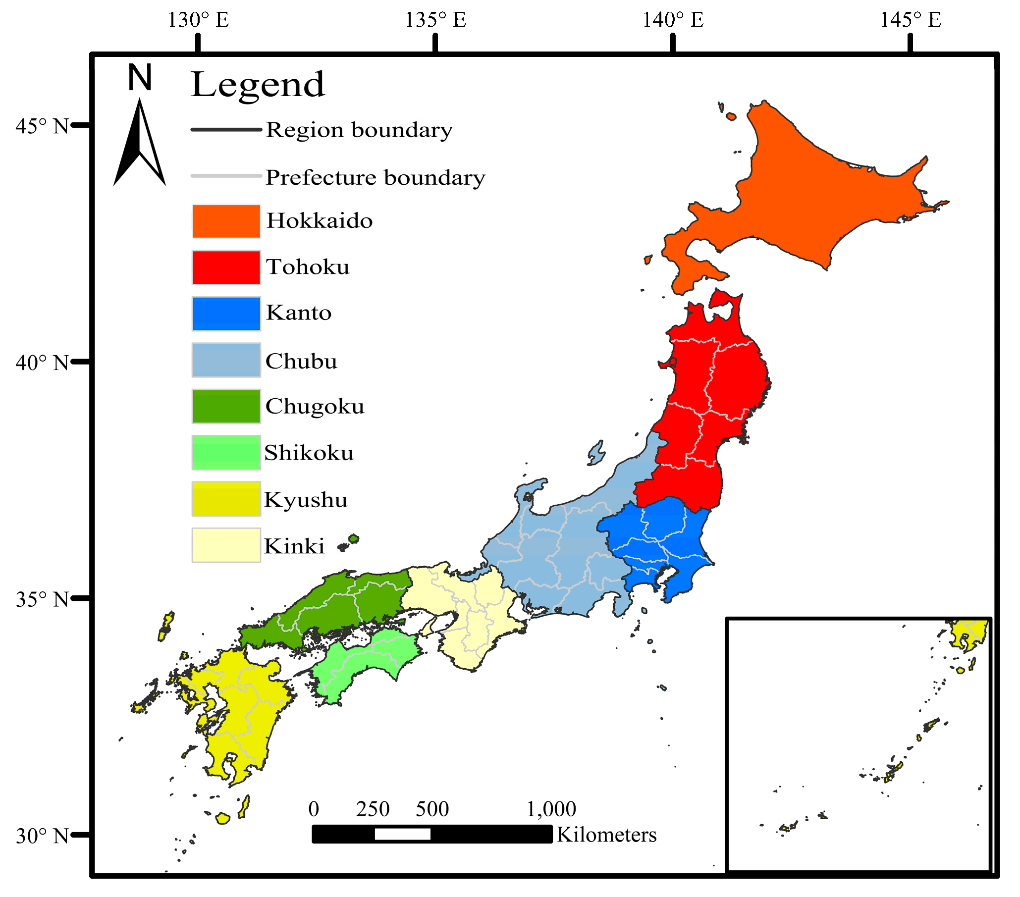
Figure 1. Regions of Japan, from north to south: Hokkaido, Tohoku, Kanto, Chubu, Kinki, Chugoku, Shikoku, and Kyushu.
Sustainability 11 06891 g001
Figure 2. Research flow chart (OLS: ordinary least squares; GWR: geographically weighted regression; SGWR: semiparametric geographically weighted regression).
Sustainability 11 06891 g002
Figure 3. The local indicators of spatial association (LISA) cluster maps of population change (HH: high-high cluster; HL: high-low outlier; LH: low-high outlier LL: low-low outlier) (a) from 2005 to 2010 and (b) from 2010 to 2015.
Sustainability 11 06891 g003
Figure 4. Parameters estimated coefficients for the local model (a) from 2005 to 2010 and (b) from 2010 to 2015.
Sustainability 11 06891 g004
Figure 5. The t-value of the parameters for the local model (a) from 2005 to 2010 and (b) from 2010 to 2015.
Sustainability 11 06891 g005
Figure 6. Local R2 based on SGWR (a) from 2005 to 2010 and (b) from 2010 to 2015.
Sustainability 11 06891 g006
Figure 7. Local estimated coefficient of underage population ratio (a) from 2005 to 2010 and (b) from 2010 to 2015.
Sustainability 11 06891 g007
Figure 8. Local estimated coefficient of ageing population ratio (a) from 2005 to 2010 and (b) from 2010 to 2015.
Sustainability 11 06891 g008
Figure 9. Local estimated coefficient of enterprise change ratio (a) from 2005 to 2010 and (b) from 2010 to 2015.
Sustainability 11 06891 g009
Table 1. Municipalities level classification.
CategoryDescriptionNumber
Large cityPopulation over 700,00021
Medium cityPopulation between 200,000 and 700,00089
Small cityPopulation below 200,000631
Town/villageMunicipality type is town or village906
Table 2. The ratio of shrinking cities classified by municipality size.
Population ChangeMunicipality Level
Large CityMedium CitySmall CityTown/Village
Continuous
shrinkage
14.3%
(3)
27.0%
(24)
70.4%
(444)
80.8%
(732)
Temporal
shrinkage
19.0%
(4)
28.1%
(25)
14.4%
(91)
10.9%
(99)
Continuous
increase
66.7%
(14)
44.9%
(40)
15.2%
(96)
8.3%
(75)
Note: Numbers in bracket refers to the counts of municipalities.
Table 3. The ratio of shrinking cities classified by region.
Population ChangeArea
HokkaidoTohokuKantoChubuKinkiChugokuShikokuKyushu
Continuous89.4%88.2%52.0%66.0%68.4%82.1%90.2%75.0%
shrinkage(160)(194)(146)(225)(134)(87)(83)(174)
Temporal7.3%6.4%19.6%17.9%15.8%8.5%4.4%13.8%
shrinkage(13)(14)(55)(61)(31)(9)(4)(32)
Continuous 3.4%5.5%28.5%16.1%15.8%9.4%5.4%11.2%
increase(6)(12)(80)(55)(31)(10)(5)(26)
Note: Numbers in bracket refers to the numbers of municipalities.
Table 4. Classification, name, and description for explanatory variables.
ClassificationNameDescription
Demographic indexesTPTotal population (people)
UPRUnderage population ratio (age < 15 years)
APRAgeing population ratio (age ≥ 65 years)
FPRForeign population ratio
Economic indexesCTPer capita taxes (JPY/people)
GRGovernment revenue (million JPY)
ECRNumbers of enterprise change ratio
STIERSecondary and tertiary industry enterprises ratio
STIWRSecondary and tertiary industry workers ratio
URUnemployment rate
Social indexesSNNumber of primary and secondary schools
HNNumber of hospitals and clinics
DNNumber of doctors (per 10,000 people)
NEFNumber of elderly facilities
NNCNumber of nursery centers
Note: The variables are computed at later years (for example, TP is the total population in year 2015 for the study period from 2010 to 2015).
Table 5. Global Moran’s I.
Study PeriodGlobal Moran’s IZ-Scorep-Value
2005–20100.46223.10<0.01
2010–20150.61530.67<0.01
Table 6. Municipality parameters estimated coefficient for the global model (R2, Coefficient of determination: AICc: corrected Akaike information criterion).
Study PeriodInterceptUPRAPRFPRECRSTIWRNNCR2Adjusted R2AICc
2005–2010−3.556*1.262*−2.907*0.315*1.029*0.0400.855*0.5250.512−5245.55
2010–2015−5.343*2.147*−1.727*0.1251.204*0.211*0.727*0.7180.715−6761.06
Note: * p < 0.05.
Table 7. Determination of parameters for the SGWR models.
Study PeriodExplanatory Variable
UPRAPRFPRECRSTIWRNNC
2005–2010LocalLocalGlobalLocalGlobalGlobal
2010–2015LocalLocalGlobalLocalGlobalGlobal
Table 8. Accuracy evaluation for the global, local, and SGWR model.
Parameter2005–20102010–2015
OLSGWRSGWROLSGWRSGWR
Bandwidth-341201-8766
Residual squares395.17 373.21 369.09 157.46 80.9477.27
AICc−5245.55 −5282.90 −5292.95 −6761.06 −7176.80 −7288.49
Adjusted R20.5120.5280.5320.7150.8150.818