A Framework for Assessing Benefits of Implemented Nature-Based Solutions

Abstract
:1. Introduction
2. Proposed Framework Overview
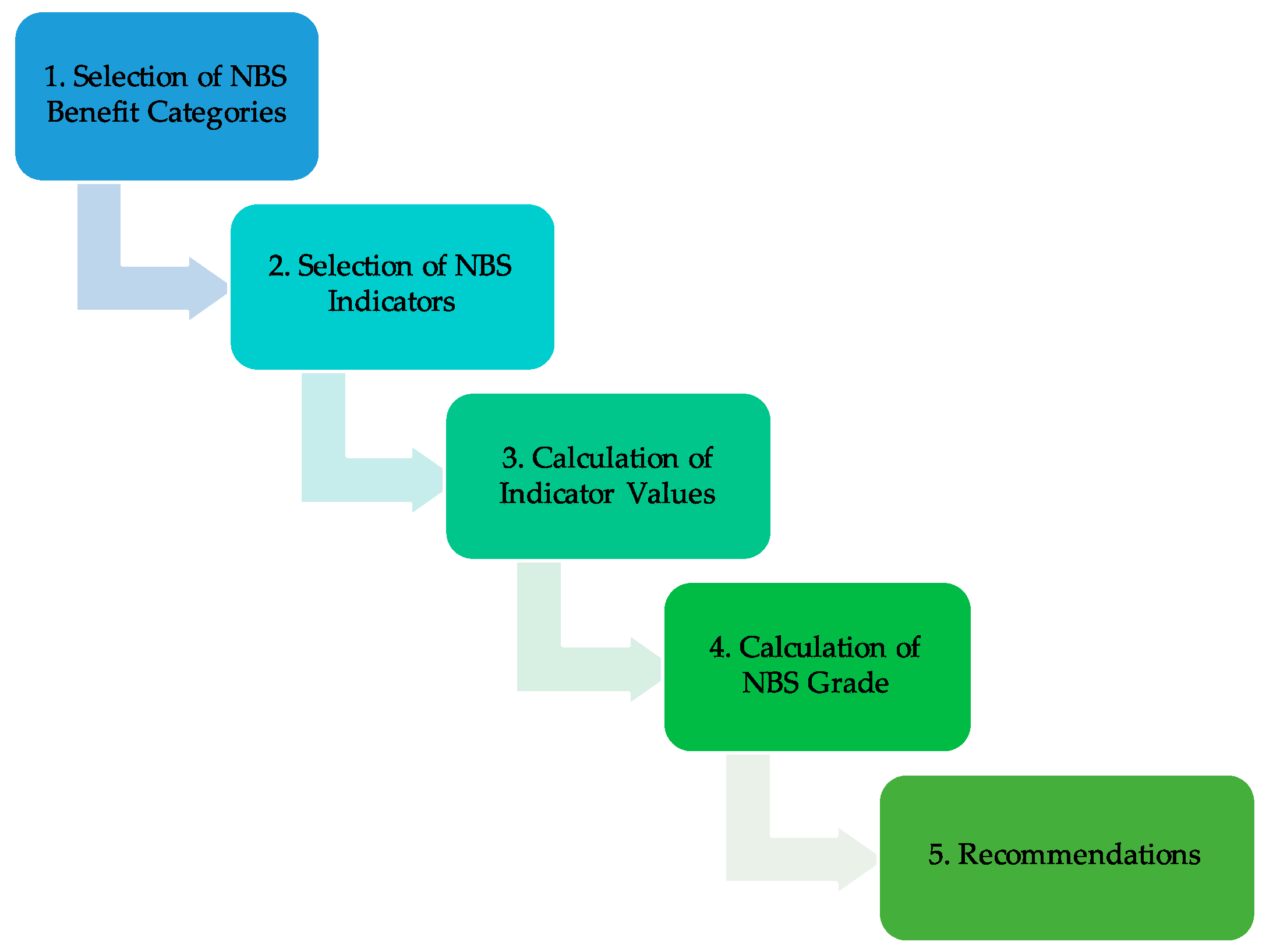
2.1. Framework Steps
2.1.1. Step 1: Selection of Benefit Categories
2.1.2. Step 2: Selection of Indicators
2.1.3. Step 3: Calculation of Indicator Values
- Percent change equation: the difference between Area A and Area B for indicator X.For positive effect, indicator: X = 100 × (A − B) ÷ AFor negative effect, indicator: X = 100 × (B − A) ÷ B
- 2
- Some indicator equations must be developed on an individual basis, these are in the category of Equation 3. These indicators may be evaluated by comparison between the NBS variable (A) and expected values, literature, other case study areas, and other methods.
2.1.4. Step 4: Calculation of NBS Grade
2.1.5. Step 5: Recommendations
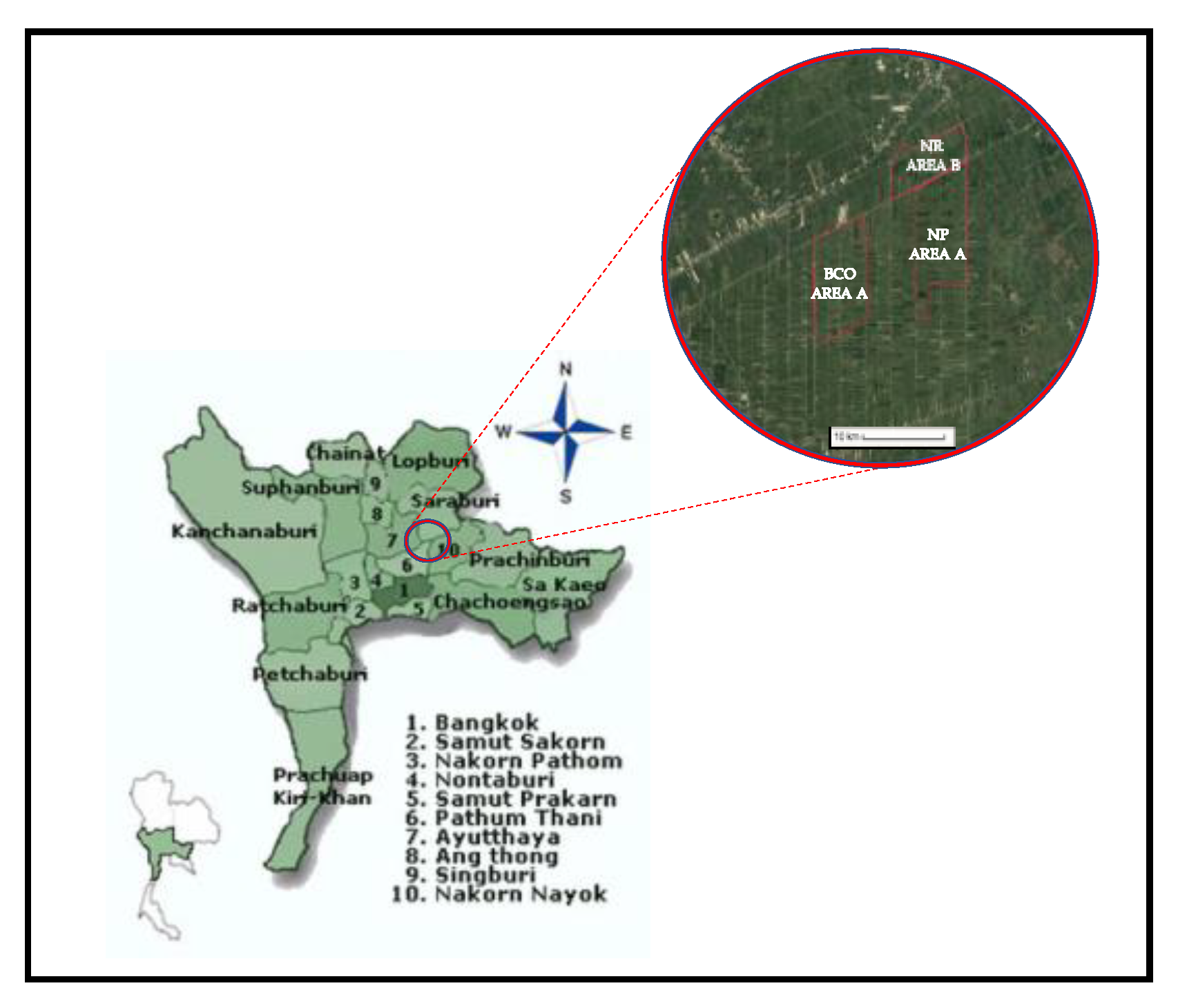
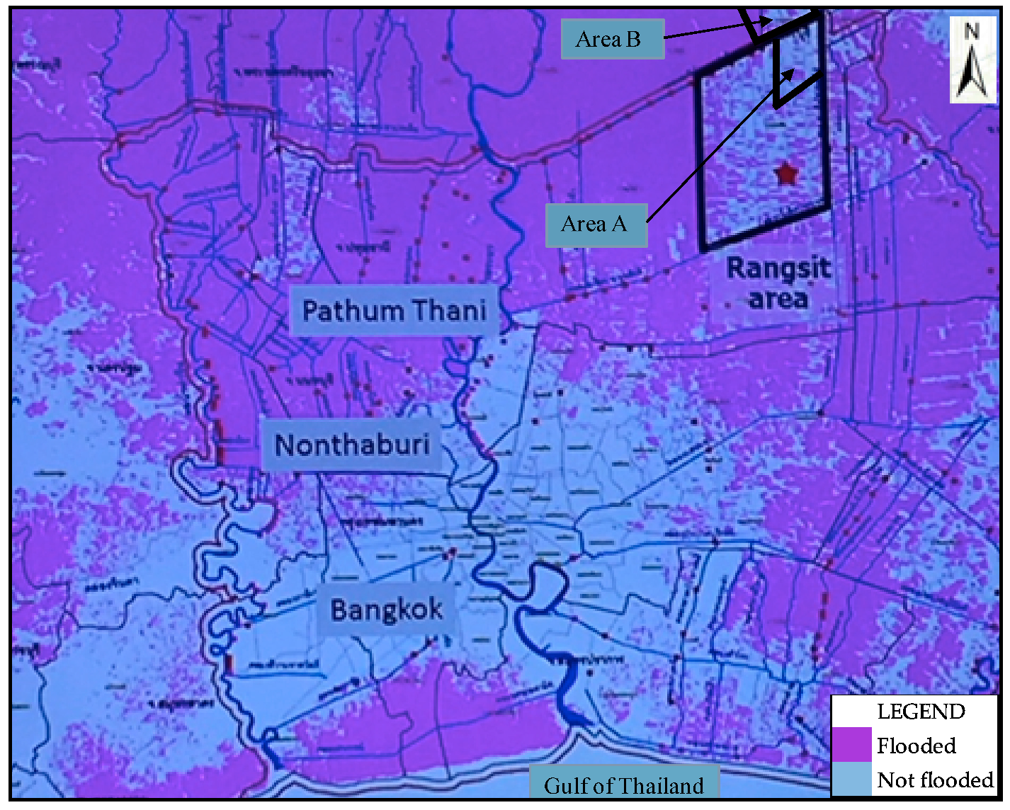
3. Framework Application: Rangsit, Thailand
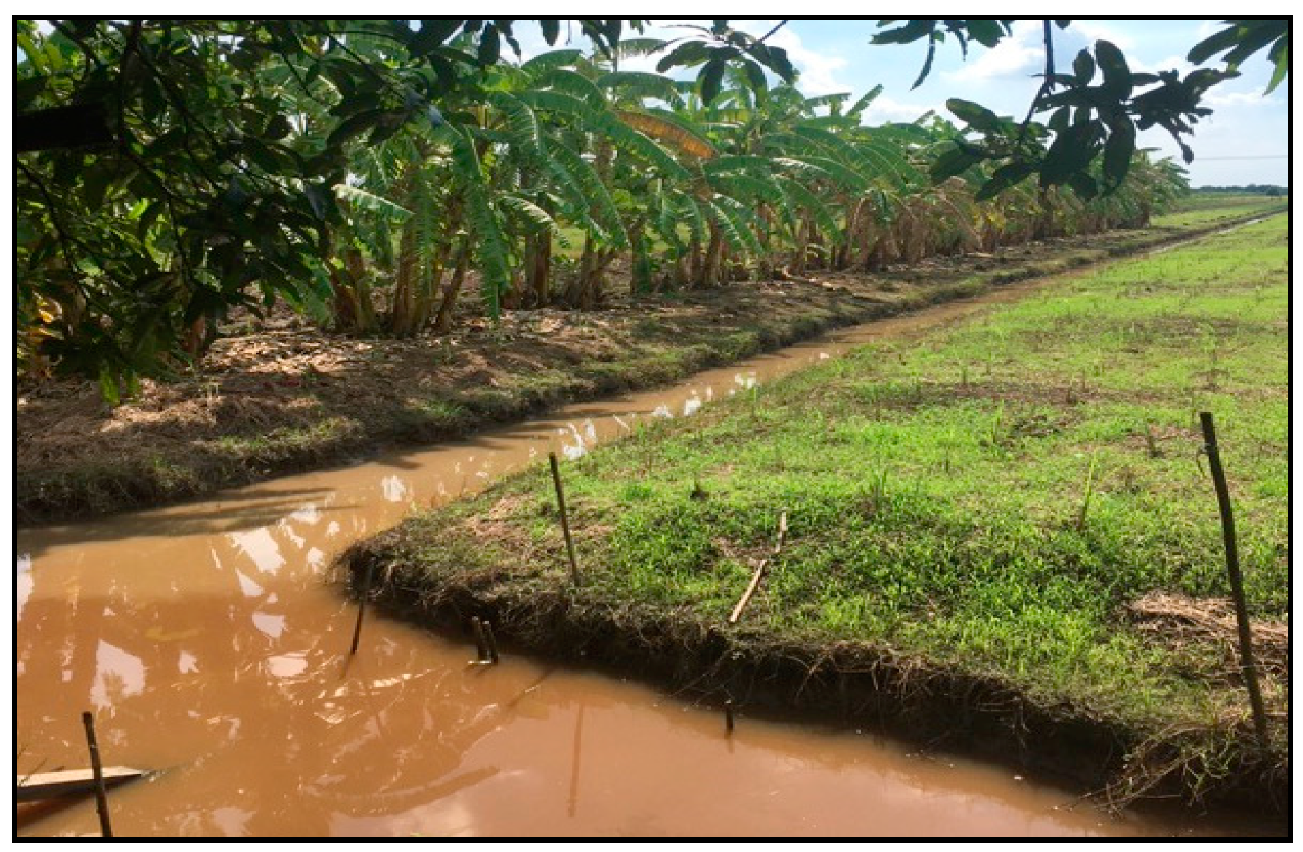
3.1. Case Study Areas
3.2. Framework Application to Rangsit Case Study Areas
3.2.1. Involvement of Stakeholders
3.2.2. Step 1: Selection of Benefit Categories
3.2.3. Step 2: Selection of Indicators
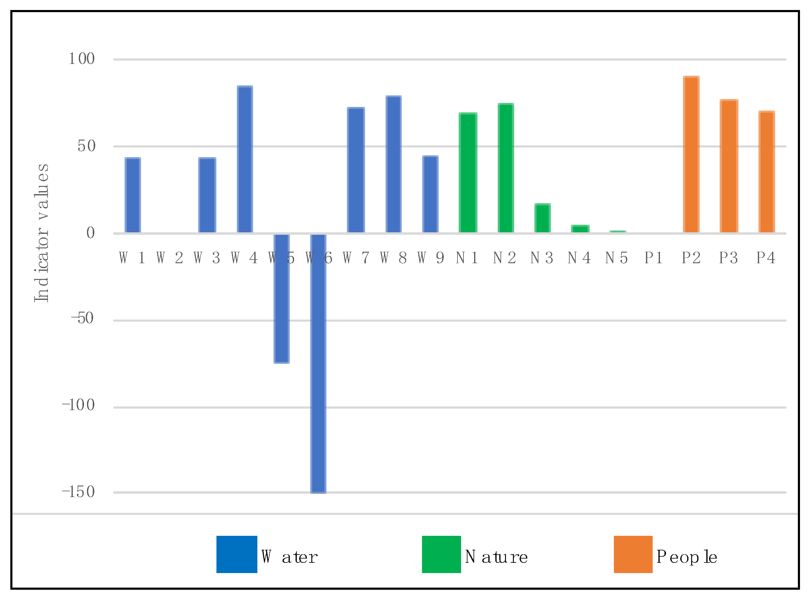
3.2.4. Step 3: Calculation of Indicator Values
3.2.5. Step 4: Calculation of NBS Grade
3.2.6. Step 5: Recommendations
4. Discussion
- Researchers who want to study the impacts from NBS on climate change;
- Water managers and planners who wish to promote, upscale, and implement NBS;
- Decision makers who may want to allocate budget for NBS construction, expansion, maintenance, and monitoring;
- Farmers who may want to improve, maintain, and expand their NBS to optimize the economic benefits;
- All stakeholders who would like to understand the full benefits of NBS.
5. Conclusions
Supplementary Materials
Author Contributions
Funding
Acknowledgments
Conflicts of Interest
References
- EM-DAT, The International Disaster Database, 2019. 2018: Extreme Weather Events Affected 60m People. Available online: https://www.unisdr.org/archive/63267 (accessed on 18 September 2019).
- Alves, A.; Gersonius, B.; Sanchez, A.; Vojinovic, Z.; Kapelan, Z. Multi-criteria approach for selection of green and grey infrastructure to reduce flood risk and increase CO-benefits. Water Resour. Manag. 2018, 32, 2505–2522. Available online: https://www.springerprofessional.de/en/multi-criteria-approach-for-selection-of-green-and-grey-infrastr/15540230 (accessed on 9 August 2019). [CrossRef]
- Dige, G.; Eichler, L.; Vermeulen, J.; Ferreira, A.; Rademaekers, K.; Adriaenssens, V.; Kolaszewska, D. Green Infrastructure and Flood Management; EEA Report; European Environment Agency: Luxembourg, 2017; Volume 14, pp. 1–156. ISBN 978-92-9213-894-3. Available online: https://www.eea.europa.eu/publications/green-infrastructure-and-flood-management (accessed on 9 November 2018).
- Vojinovic, Z.; Keerakamolchai, W.; Weesakul, S.; Pudar, R.S.; Medina, N.; Alves, A. Combining ecosystem services with cost-benefit analysis for selection of green and grey infrastructure for flood protection in a cultural setting. Environments 2017, 4, 3. Available online: https://www.mdpi.com/2076-3298/4/1/3/htm (accessed on 9 July 2019). [CrossRef]
- Alves, A.; Sanchez, A.; Vojinovic, Z.; Seyoum, S.; Babel, M.; Brdjanovic, D. Evolutionary and holistic assessment of Green-Grey infrastructure for CSO reduction. Water 2016, 8, 402. Available online: https://www.mdpi.com/2073-4441/8/9/402 (accessed on 9 July 2019). [CrossRef]
- Zhao, H.; Zhao, J.; Li, X.; Zou, C. Role of Low-Impact developments in generation and control of urban diffuse pollution in a pilot sponge city: A Paired-Catchment study. Water 2018, 10, 852. Available online: https://www.mdpi.com/2073-4441/10/7/852 (accessed on 9 November 2018). [CrossRef]
- Keesstra, S.D.; Kondrlova, E.; Czajka, A.; Seeger, M.; Maroulis, J. Assessing riparian zone impacts on water and sediment movement: A new approach. Neth. J. Geosci. 2012, 91, 245–255. Available online: https://www.cambridge.org/core/journals/netherlands-journal-of-geosciences/article/assessing-riparian-zone-impacts-on-water-and-sediment-movement-a-new-%20approach/62A646C5709A49E3CE6B38A39926A03B (accessed on 21 December 2018). [CrossRef]
- Martinez, C.; Sanchez, A.; Galindo, R.; Mulugeta, A.; Vojinovic, Z.; Galvis, A. Configuring Green Infrastructure for Urban Runoff and Pollutant Reduction Using an Optimal Number of Units. Water 2018, 10, 1528. Available online: https://www.mdpi.com/2073-4441/10/11/1528 (accessed on 9 July 2019). [CrossRef]
- Roy, A.H.; Wenger, S.J.; Fletcher, T.D.; Walsh, C.J.; Ladson, R.A.; Shuster, W.D.; Thurston, H.W.; Brown, R.R. Impediments and solutions to sustainable, watershed-scale urban stormwater management: Lessons from Australia and US. Environ. Manag. 2012, 42, 344–359. Available online: https://link.springer.com/article/10.1007/s00267-008-9119-1 (accessed on 10 November 2018). [CrossRef] [PubMed]
- Dutch Water Sector (DWS). Boskalis Contracted for Dutch Room for the River Project at Veessen-Wapenveld, the Netherlands. Dutch Water Sector. 4 July 2013. Available online: https://www.dutchwatersector.com/news/boskalis-contracted-for-dutch-room-for-the-river-project-at veessen-wapenveld-the-netherlands (accessed on 5 November 2018).
- EPA. Healthy Benefits of Green Infrastructure in Communities. 2017. Available online: https://www.epa.gov/sites/production/files/2017-11/documents/greeninfrastructure_healthy_communities_factsheet.pdf#targetText=Green%20infrastructure%20installments%20also%20provide,overall%20health%20and%20well%2Dbeing (accessed on 5 November 2018).
- Lawson, E.; Thorne, C.; Ahilan, S.; Allen, D.; Arthur, S.; Everett, G.; Fenner, R.; Glenis, V.; Guan, D.; Hoang, L.; et al. Delivering and evaluating the multiple flood risk benefits in blue-green cities: An interdisciplinary approach. WIT Trans. Ecol. Environ. 2014, 184, 113–124. Available online: https://www.witpress.com/elibrary/wit-transactions-on-ecology-and-the-environment/184/28342 (accessed on 12 December 2018).
- Zhang, J.; Yu, Z.; Yu, T.; Si, J.; Feng, Q.; Cao, S. Transforming flash floods into resources in arid China. Land Use Policy 2018, 76, 746–753. Available online: https://www.sciencedirect.com/science/article/abs/pii/S0264837717314102 (accessed on 5 November 2018). [CrossRef]
- World Bank Implementing Nature-Based Flood Protection: Principles and Implementation Guidance. 2017. Available online: http://documents.worldbank.org/curated/en/739421509427698706/%20Implementing-nature-based-flood-protection-principles-and-implementation-guidance (accessed on 21 December 2018).
- Ruangpan, L.; Vojinovic, Z.; Di Sabatino, S.; Leo, L.S.; Capobianco, V.; Oen, A.M.P.; McClain, M.; Lopez-Gunn, E. Nature-Based Solutions for Hydro-meteorological Risk Reduction: A State-of-the-art review of the research area. Nat. Hazards Earth Syst. Sci. 2019. under review. Available online: https://www.nat-hazards-earth-syst-sci-discuss.net/nhess-2019-128/ (accessed on 9 August 2019).
- Alves, A.; Gersonius, B.; Kapelan, Z.; Vojinovic, Z.; Sanchez, A. Assessing the Co-Benefits of Green-blue-grey infrastructure for sustainable flood risk management. J. Environ. Manag. 2019, 239, 244–254. Available online: https://www.deepdyve.com/lp/elsevier/assessing-the-co-benefits-of-green-blue-grey-infrastructure-for-qnphUg7fuW?impressionId=5d059af1a1edf&i_medium=docview&i_campaign=recommendations&i_source=recommendations (accessed on 9 August 2019). [CrossRef] [PubMed]
- Raymond, C.M.; Berry, P.; Breil, M.; Nita, M.R.; Kabisch, N.; de Bel, M.; Enzi, V.; Frantzeskaki, N.; Geneletti, D.; Cardinaletti, M.; et al. An Impact Evaluation Framework to Support Planning and Evaluation of Nature-based Solutions Projects; EKLIPSE Expert Working Group on Nature-based Solutions to Promote Climate Resilience in Urban Areas; Centre for Ecology & Hydrology: Wallingford, UK, 2017; Available online: http://www.eklipse-mechanism.eu/apps/Eklipse_data/website/EKLIPSE_Report1-NBS_FINAL_Complete-08022017_LowRes_4Web.pdf (accessed on 12 September 2018).
- Thorne, C.R.; Lawson, E.C.; Ozawa, C.; Hamlin, S.L.; Smith, L.A. Overcoming uncertainty and barriers to adoption of Blue-Green infrastructure for urban flood risk management. J. Flood Risk Manag. 2018, 11, S960–S972. Available online: https://onlinelibrary.wiley.com/doi/full/10.1111/jfr3.12218 (accessed on 28 October 2018). [CrossRef]
- Shinde, R.; Babel, M.S.; Suttharom, P. Manual on Framework for River Health Assessment in Thailand 2018. Asian Institute of Technology: Bangkok, Thailand. Available online: https://cgspace.cgiar.org/bitstream/handle/10568/92848/Frame%20work%20for%20River%20Health%20in%20Thailand.pdf?sequence=1&isAllowed=y (accessed on 5 November 2018).
- RECONECT Project Objectives. Available online: http://www.reconect.eu/about-reconect/ (accessed on 6 November 2019).
- Suksumek, T. Central Thailand. Weebly 2014. Available online: https://hgq2.weebly.com/central-region. https://hgq2.weebly.com/ (accessed on 18 November 2018).
- Ditthabumrung, S. Nature-Based Solutions for Water Management: A Case Study in The Rangsit Area, Thailand; AIT Thesis No. WEM-18-08; Asian Institute of Technology: Bangkok, Thailand, 2018. [Google Scholar]
- Carr, M.K.V. The Water Relations and Irrigation Requirements of Oil Palm (Elaeis Guineensis): A review. Expl. Agric. 2011, 47, 629–652. Available online: http://agris.fao.org/agris-search/search.do?recordID=US201500053138 (accessed on 22 October 2019). [CrossRef]
- World Bank Group. Climate Data Historical Page. Available online: https://climateknowledgeportal.worldbank.org/country/thailand/climate-data-historical (accessed on 20 October 2019).
- Tantivejkul, S. Application of Science and Technology for Community Water-Related Disaster Risk Reduction; Utokapat Foundation Under the Royal Patronage of H.M. the King; Hydro and Agro Informatics Institute (HAII): Bangkok, Thailand, 2016. [Google Scholar]
- Huizinga, J.; de Moel, H.; Szewczyk, W. Global Flood Depth-Damage Functions. JCR Technical Reports 2017; European Commission. EUR 28552 EN. Available online: https://publications.jrc.ec.europa.eu/repository/bitstream/JRC105688/global_flood_depth-damage_functions__10042017.pdf (accessed on 12 February 2019). [CrossRef]
- Couto, T.B.A.; Zuanon, J.; Olden, J.D.; Ferraz, G. Longitudinal variability in lateral hydrologic connectivity shapes fish occurrence in temporal floodplain ponds. Can. J. Fish. Aquat. Sci. 2017, 72, 319–328. Available online: https://tspace.library.utoronto.ca/bitstream/1807/78869/1/cjfas-2016-0388.pdf (accessed on 2 September 2018).
- The National Committee on Irrigation and Drainage (THAICID). 1999. Thailand. Available online: http://www.rid.go.th/thaicid/_5_article/article_body_1th.php (accessed on 23 November 2018).
- Fornes, J.; Pirarai, K. Groundwater in Thailand. J. Environ. Sci. Eng. 2014, 3, 304–315. Available online: http://www.davidpublisher.org/Public/uploads/Contribute/55078898cb5e0.pdf (accessed on 23 November 2018).
- Sydney Water Corporation. Stage—Primary Treatment; Wastewater Treatment Plant Virtual Tour. 2010. Available online: https://www.sydneywater.com.au/Education/Tours/virtualtour/html/primary-treatment.html (accessed on 18 November 2018).
- Poomkhonsan, N.; Konyai, S. Land Use and Hydrologic Soil Group Classification for the Yang River Basin in Northeast Thailand. KKU Eng. J. 2013, 40, 473–483. Available online: https://www.tci- thaijo.org/index.php/easr/article/view/21735 (accessed on 25 November 2018).
- Rawls, M.; Brakensiek, D.L.; Miller, N. Green-ampt Infiltration Parameters from Soils Data. J. Hydraul. Eng. 1983, 109, 62. Available online: https://ascelibrary.org/doi/pdf/10.1061/%28ASCE%290733-9429%281983%29109%3A1%2862%29 (accessed on 9 December 2018). [CrossRef]
- Chavez, C. (USDA). Soil Infiltration Ability to Take in Water 2010 PowerPoint presentation. Available online: https://prod.nrcs.usda.gov/Internet/FSE_DOCUMENTS/nrcs144p2_068436.pdf (accessed on 8 December 2018).
- Puttaso, A.; Vityakon, P.; Trelo-ges, V.; Saenjan, P.; Cadisch, G. Effect of Long-Term (13 Years) Application of Different Quality Plant Residues on Soil Organic Carbon and Soil Properties of Sandy Soil of Northeast Thailand. KKU Res. J. 2011, 16, 359–370. Available online: https://www.researchgate.net/publication/225968734_Relationship_between_residue_quality_decomposition_patterns_and_soil_organic_matter_accumulation_in_a_tropical_sandy_soil_after_13_years (accessed on 12 November 2018).
- Zhang, W.; Dulloo, E.; Kennedy, G.; Bailey, A.; Sandhu, H.; Nkonya, E. Biodiversity and ecosystem services. In Sustainable Food and Agriculture An Integrated Approach; Campanhola, C., Pandey, S., Eds.; Academic Press: Rome, Italy, 2019; Chapter 8; pp. 137–152. ISBN 978-0-12-812134-4. [Google Scholar]
- Lal, R. Carbon emission from farm operations. Environ. Int. 2004, 30, 981–990. Available online: https://www.sciencebase.gov/catalog/item/5140be35e4b06685e5db9794 (accessed on 21 December 2018). [CrossRef]
- ESA. Sentinel-5P NRTI NO2: Near Real-Time Nitrogen Dioxide Data 2018. Available online: https://sentinel.esa.int/web/sentinel/user-guides/sentinel-5p-tropomi (accessed on 22 January 2019).
- Delshammar, T. NBS Case Study: Malmo. Think Nature Platform Case Studies 2018. Available online: https://platform.think-nature.eu/nbs-case-study/19011 (accessed on 23 November 2018).


| Type of Equation | Related Indicators | |
|---|---|---|
| Equation (1): positive effects | Connectivity GWR Biodiversity Habitat provision Carbon storage Cultural and spiritual | Community interaction and development Aesthetics/property value Agriculture Economic Green jobs |
| Equation (2): negative effects | Historical flood mitigation Coastal flood mitigation Resilience to drought Resilience to flood Irrigation costs | Air quality Water quality Climate control Landslide risk reduction Noise quality |
| Equation (3): comparison of indicator values with the literature or case studies | Research Infiltration Recreational | Education Quality of life Social safety |
| Indicator Value | Score |
|---|---|
| <20 | 1 |
| 20–40 | 2 |
| 40–60 | 3 |
| 60–80 | 4 |
| >80 | 5 |
| NBS Grade | Description | Grade Number |
|---|---|---|
| Very poor | The NBS do not provide any benefits; re-evaluation is necessary. | 0–1 |
| Poor | The NBS are providing very few benefits; improvements may be required; re-evaluation may be necessary. | 1–2 |
| Good | The NBS are providing some added benefits; some improvements may be required. | 2–3 |
| Very good | The NBS are providing added benefits; minor improvements may be required. | 3–4 |
| Excellent | The NBS are adding at least 80% more benefits; continue with regular maintenance. | 4–5 |
| Indicator | Reasons for Selection | Data Source |
|---|---|---|
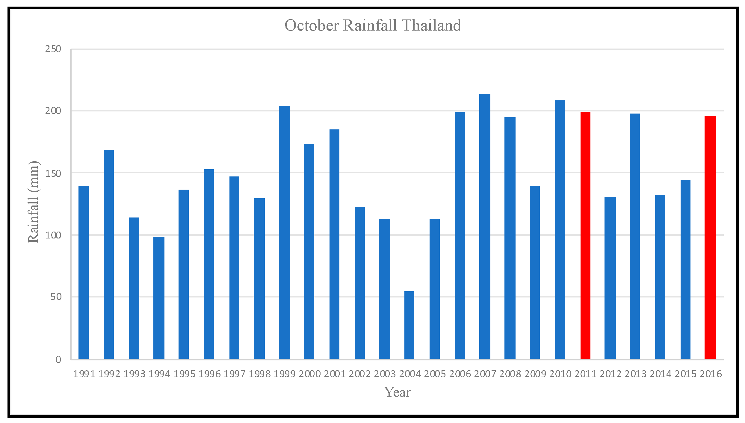
| W1: Local flood mitigation W2: Downstream flood mitigation | Occurrence of past flood event (2016). Hydrodynamic model for Rangsit was available. | World Bank database (rainfall) |
| W3: Historical flood mitigation | Occurrence of past flood event (2011). | 2011 Flood map |
| W4: Water storage and reuse | Dimensions of the furrows, storage capacity, and furrow water use information were available. | Previous research [22] Farmer interviews |
| W5: Irrigation cost | Irrigation costs were available. | Farmer and government expert (irrigation department) interviews |
| W6: Resiliency to drought | Incomes in drought and non-drought years were available. | Farmer interviews |
| W7: Connectivity | Aerial images were available. | Google Earth |
| W8: GWR | Rainfall data and groundwater monitoring well level data were available. Declining groundwater level was a concern in Thailand. | World Bank database (rainfall) Government expert interview (groundwater resources) |
| W9: Water quality | Water sampling locations, and TSS and turbidity measuring equipment were available. | In-situ sampling |
| N1: Infiltration | Test locations and infiltration rings were available. | In-situ sampling |
| N2: Biodiversity | Species information was available. | Farmer and municipality interviews |
| N3: Soil quality | Soil sampling locations and a testing laboratory were available. | In-situ sampling |
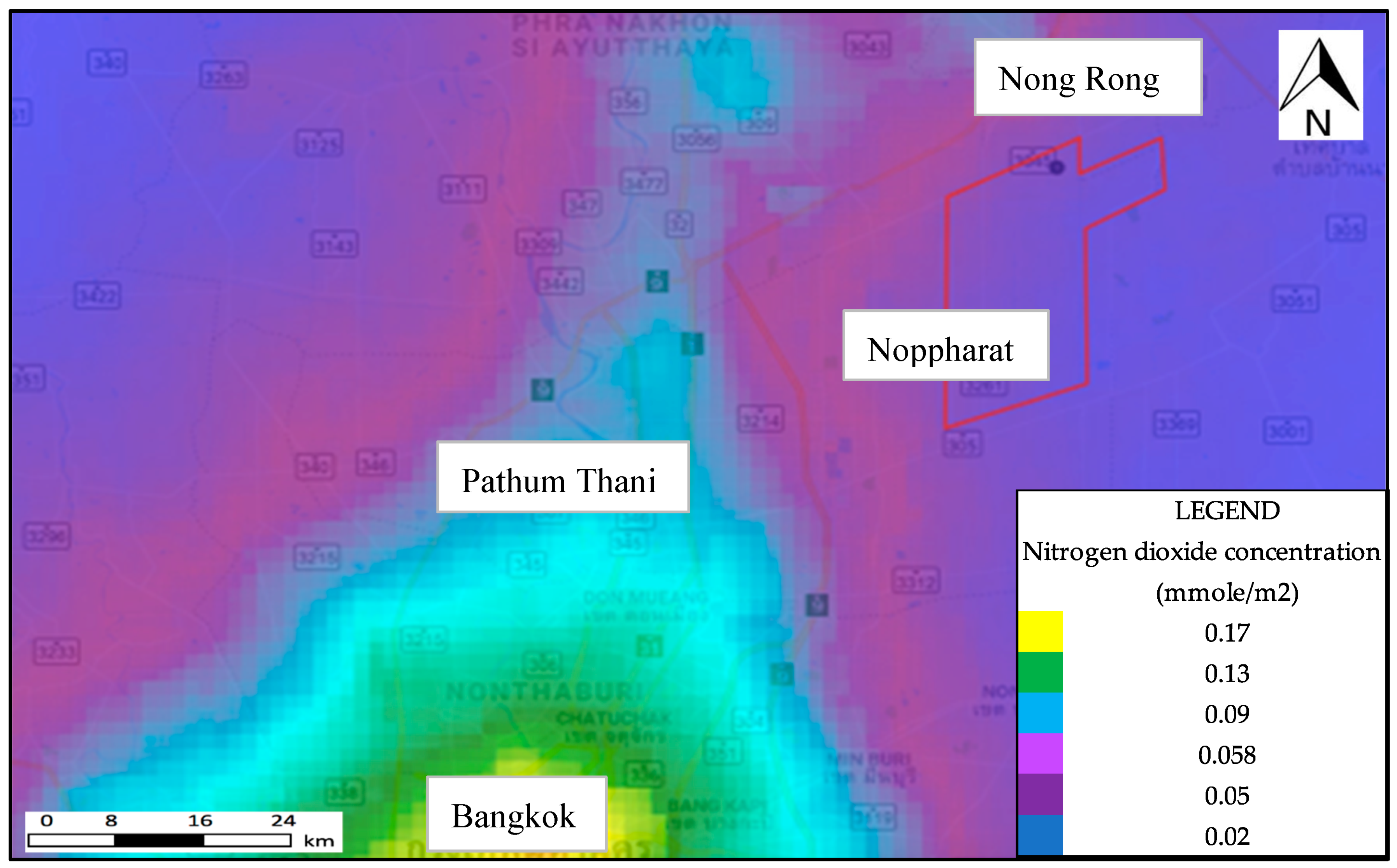
| N4: Fertilizer reduction N5: Air quality | Fertilizer use and carbon emission information were available. | Farmer interviews |
| P1: Cultural and spiritual P2: Education and research | Number of events were available. | Farmer and municipality interviews |
| P3: Economic P4: Agricultural | Annual incomes and expenses information were available. | Farmer interviews |
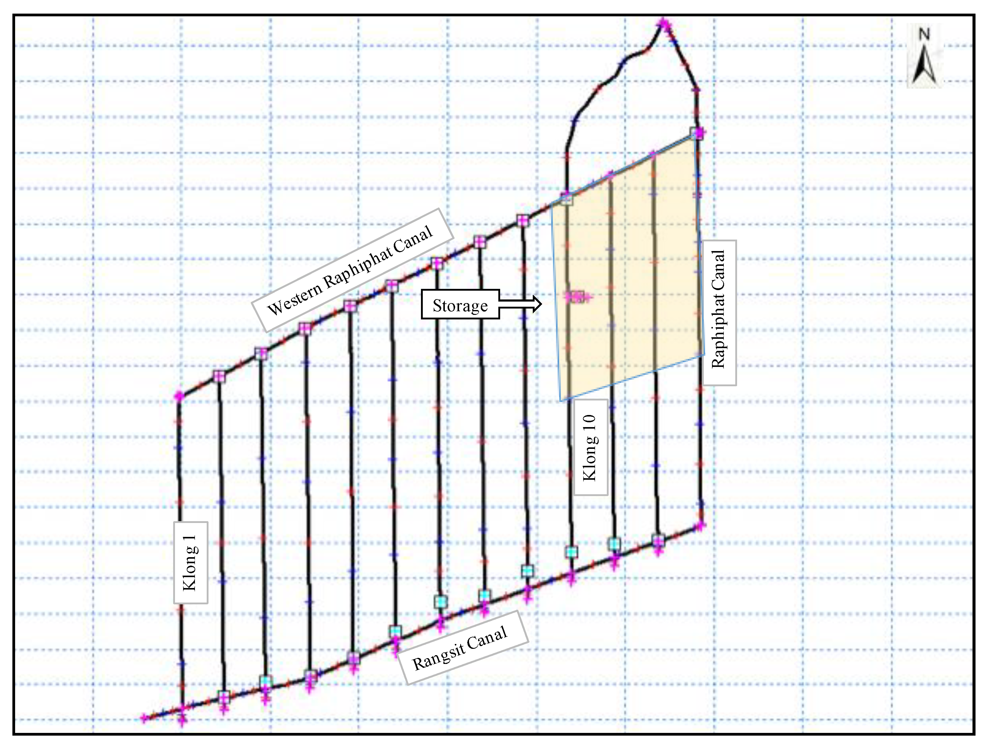
| Cross-Section | A. Top Canal Bank (m) | B. Max Water Level (No Storage) (m) | C. Height Difference (m) A–B | D. Max Water Level (with Storage) (m) | E. Height Difference (m) A–D | Flood Height Reduction (m) C–E |
|---|---|---|---|---|---|---|
| K10-1 | 3.828 | 5.246 | −1.418 * | 5.031 | −1.203 * | −0.215 |
| K10-2 | 3.593 | 5.246 | −1.653 * | 5.03 | −1.437 * | −0.216 |
| K10-3 | 3.6 | 5.246 | −1.646 * | 5.03 | −1.43 * | −0.216 |
| K10-4 | 3.767 | 5.246 | −1.479 * | 5.03 | −1.263 * | −0.216 |
| K10-5 | 3.136 | 5.246 | −2.11 * | 5.03 | −1.894 * | −0.216 |
| Average flood height reduction due to the addition of storage: | −0.216 | |||||
| D (height of maximum damage from depth-damage curve) = 0.5 m Hst (flood height reduction with NBS storage) = 0.216 m | ||||||
| W1 = 100 [1 − (D − Hst) ÷ D] = 100 [1 − (0.5 − 0.216) ÷ 0.5] = 43 | ||||||
| Cross-Section | A. Top Canal Bank (m) | B. Max Water Level (No Storage) (m) | C. Height Difference (m) A–B | D. Max Water Level (with Storage) (m) | E. Height Difference (m) A–D | Flood Height Reduction (m) C–E |
|---|---|---|---|---|---|---|
| K1-1 | 3.684 | 3.392 | 0.292 | 3.392 | 0.292 | 0 |
| K1-2 | 3.684 | 3.286 | 0.398 | 3.286 | 0.398 | 0 |
| K1-3 | 2.319 | 3.004 | −0.685 * | 3.004 | −0.685 * | 0 |
| K1-4 | 2.834 | 1.971 | 0.863 | 1.971 | 0.863 | 0 |
| K1-5 | 1.836 | 1.499 | 0.337 | 1.499 | 0.337 | 0 |
| Average flood height reduction due to the addition of storage: | 0 | |||||
| D (height of maximum damage from depth-damage curve) = 0.5 m Hst (flood height reduction with NBS storage) = 0 m W2 = 100 [1 − (D − Hst) ÷ D] = 100 [1 − (0.5 − 0) ÷ 0.5] = 0 | ||||||
| Farm | Irrigation Cost and Units | Farm Size (Rai) | Irrigation Cost (Baht/year/Rai) |
|---|---|---|---|
| A-3 | 350 Baht/week | 18 | 1011 |
| A-4 | 1750 Baht/month | 18 | 1167 |
| Average Area A farms (A): | 1089 | ||
| B-1 | 12,000 Baht/year | 36 | 333 |
| B-2 | 12,000 Baht/year | 9 | 1333 |
| B-3 | 24,000 Baht/year | 36 | 670 |
| B-4 | 1250 Baht/year | 8.3 | 150 |
| Average Area B farms (B): | 622 | ||
| W5 = 100 [(B − A) ÷ B] = 100 [(622 − 1089) ÷ 622] = −75 | |||
| Farm | Loss of Income (%) |
|---|---|
| A-3 | 0 |
| A-4 | 30 |
| Average Area A farms (A): 15 | |
| B-1 | 50 |
| B-2 | 20 |
| B-3 | 20 |
| B-4 | −67 (gain) |
| Average Area B farms (B): 6 | |
| W6 = 100 [(B − A) ÷ B] = 100 [(6 − 15) ÷ 6] = −150 | |
| Area | (1) Length of Canals (km) | (2) Length of Furrows (km) | (3) Area of Sub-District (km2) | Total Length Per Area (km/km2) [(1) + (2)] ÷ (3) |
|---|---|---|---|---|
| A | 51.12 | 254.80 | 66.1 | 4.63 (A) |
| B | 34.3 | 0 | 26.7 | 1.28 (B) |
| W7 = 100 [(A − B) ÷ A] = 100 [(4.63 − 1.28) ÷ 4.63] = 72 | ||||
| Parameter | Furrows A-1 to A-4 (A) | K12 Canal (K) | [(Wi,K − Wi,A) ÷ Wi,K] |
|---|---|---|---|
| Average TDS (ppm) | 453 | 291 | 0.36 |
| Average turbidity (NTU) | 86 | 39 | 0.55 |
| W9 = average [(Wi,K − Wi,A) ÷ Wi,K] 100 = average (0.36, 0.55) 100 = 45 | |||
| Infiltration Method | Infiltration Rate (mm/hour) | |
|---|---|---|
| Using site parameters (A) | Infiltration rings | 7.5 (average of 6, 9) |
| Green Ampt | 10.2 (see Table S7) | |
| Literature | 10.0 [33] | |
| Average A: | 9.2 | |
| Desired infiltration (L) | Literature | 13.3 [34] |
| N1 = 100 [1 − {(L − A) ÷ L}] = 100 [1 − {(13.3 − 9.2) ÷ 13.3}] = 69 | ||
| Farm | Sample Type | Total Nitrogen (%) | Total Phosphorus (%) | Total Potassium (%) |
|---|---|---|---|---|
| A-3 | Sediment (S) | 0.5 | 0.5 | 0.25 |
| Soil (N) | not detected | 0.6 | 0.22 | |
| A-4 | Sediment (S) | 0.5 | 0.5 | 0.19 |
| Soil (N) | 0.5 | 0.5 | 0.22 | |
| Average sediment (S): | 0.5 | 0.5 | 0.22 | |
| Average soil (N): | 0.25 | 0.5 | 0.22 | |
| [(Zi,S − Zi,N) ÷ Zi,S]: | 50 | 0 | 0 | |
| N3 = average [(Zi,S − Zi,N) ÷ Zi,S]: average (50,0,0) = 17 | ||||
| Farm | Farm Area (Rai) | Baht/Year | Kg Fertilizer/Year | Kg Fertilizer/Year/Rai |
|---|---|---|---|---|
| A-3 | 18 | 5000 | 250 | 14 |
| A-4 | 18 | 30,000 | 1500 | 83 |
| Average Area A farms (A): 49 | ||||
| B-1 | 36 | 28,800 | 1440 | 40 |
| B-2 | 9 | 13,400 | 670 | 74 |
| B-3 | 36 | 32,000 | 1600 | 44 |
| B-4 | 8.3 | 7470 | 374 | 45 |
| Average Area B farms (B): 51 | ||||
| N4 = 100 (B − A) ÷ B = 100 (51 − 49) ÷ 52 = 5 | ||||
| Farm | Income (Baht/Year/km2) |
|---|---|
| A-3 | 27,778 |
| A-4 | 22,222 |
| Average Area A farms (A): 25,000 | |
| B-1 | 4089 |
| B-2 | 12,222 |
| B-3 | 6667 |
| B-4 | 361 |
| Average Area B farms (B): 5835 | |
| P3 = 100 (A − B) ÷ A = 100 (25,000 − 5835) ÷ 25,000 = 77 | |
| Location | Income (Baht/Year/km2) | Expenses (Baht/Year/km2) | Productivity (Income/Expenses) |
|---|---|---|---|
| A-3 | 27,778 | 1667 | 25,000/3611 = 6.9 |
| A-4 | 22,222 | 5556 | |
| Average A: | 25,000 | 3611 | |
| B-1 | 4089 | 4000 | 5835/2848 = 2.0 |
| B-2 | 12,222 | 4444 | |
| B-3 | 6667 | 2778 | |
| B-4 | 361 | 169 | |
| Average B: | 5835 | 2848 | |
| P4 = 100 (A − B) ÷ A = 100 (6.9 − 2.0) ÷ 6.9 = 70 | |||
| Category | Indicators | Weight |
|---|---|---|
| Safety | Local flood mitigation | 0.45 |
| Downstream flood mitigation | ||
| Historical flood mitigation | ||
| Income | Economic | 0.30 |
| Agricultural | ||
| Irrigation cost | ||
| Resiliency to flood | ||
| Environmental improvement | Water storage and reuse | 0.15 |
| Connectivity | ||
| Infiltration | ||
| GWR | ||
| Biodiversity | ||
| Soil quality | ||
| Fertilizer reduction | ||
| Air quality | ||
| Water quality | ||
| Pastime | Cultural/spiritual | 0.10 |
| Education and research |
| Indicator | Name | Calculated Value | Score (Using Table 2) | Average Score | Weight | Weighted Average Score (Average Score × Weight) |
|---|---|---|---|---|---|---|
| W1 | Local flood mitigation | 43 | 3 | 3 | 0.45 | 1.35 |
| W2 | {Downstream flood mitigation} | {0} | {0} | |||
| W3 | Historical flood mitigation | 44 | 3 | |||
| P3 | Economic | 77 | 4 | 4 | 0.3 | 1.2 |
| P4 | Agricultural | 70 | 4 | |||
| W5 | {Irrigation cost} | {−75} | {1} | |||
| W6 | {Resiliency to flood} | {−150} | {1} | |||
| W4 | Water storage and reuse | 85 | 5 | 4 | 0.15 | 0.6 |
| W7 | Connectivity | 72 | 4 | |||
| N1 | Infiltration | 69 | 4 | |||
| W8 | GWR | 79 | 4 | |||
| N2 | Biodiversity | 75 | 4 | |||
| N3 | {Soil quality} | {17} | {1} | |||
| N4 | {Fertilizer reduction} | {4} | {1} | |||
| N5 | {Air quality} | {1} | {1} | |||
| W9 | Water quality | 45 | 3 | |||
| P1 | {Cultural/spiritual} | {0} | {0} | 0.5 | ||
| P2 | Education and research | 90 | 5 | 5 | 0.1 | |
| Furrow grade (sum of weighted scores): | 3.65 | |||||
| Indicator | Recommendations |
|---|---|
| W1 Flood mitigation: local, rural | Flood preparedness
Implement furrows in other areas |
| W2 Flood mitigation: downstream, urban | Increase water storage capacity
|
| W3 Flood mitigation: historical | Improve flood water storage capacity
|
| W4 Water storage and reuse | Increase the storage capacity
Use more efficient irrigation methods |
| W5 Irrigation cost | Reduce irrigation costs
|
| W6 Resiliency | Increase drought resiliency
|
| W7 Connectivity | Improve water connectivity
|
| W8 GWR | Improve GWR
|
| W9 Water quality | Improve water quality
|
| N1 Infiltration | Increase infiltration
|
| N2 Biodiversity | Increase biodiversity
|
| N3 Soil quality: nutrients | Improve soil quality
|
| N4 Soil quality: fertilizer use | Reduce fertilizer use
|
| N5 Air quality | Reduce pollutants
|
| P1 Cultural and spiritual | Discuss the benefits of furrows with community members |
| P2 Education and research | Continue to promote the use of furrows to others |
| P3 Economic: Incomes | Improve crop yield
|
| P4 Agricultural productivity | Improve productivity
|
© 2019 by the authors. Licensee MDPI, Basel, Switzerland. This article is an open access article distributed under the terms and conditions of the Creative Commons Attribution (CC BY) license (http://creativecommons.org/licenses/by/4.0/).
Share and Cite
Watkin, L.J.; Ruangpan, L.; Vojinovic, Z.; Weesakul, S.; Torres, A.S. A Framework for Assessing Benefits of Implemented Nature-Based Solutions. Sustainability 2019, 11, 6788. https://doi.org/10.3390/su11236788
Watkin LJ, Ruangpan L, Vojinovic Z, Weesakul S, Torres AS. A Framework for Assessing Benefits of Implemented Nature-Based Solutions. Sustainability. 2019; 11(23):6788. https://doi.org/10.3390/su11236788
Chicago/Turabian StyleWatkin, Linda J., Laddaporn Ruangpan, Zoran Vojinovic, Sutat Weesakul, and Arlex Sanchez Torres. 2019. "A Framework for Assessing Benefits of Implemented Nature-Based Solutions" Sustainability 11, no. 23: 6788. https://doi.org/10.3390/su11236788
APA StyleWatkin, L. J., Ruangpan, L., Vojinovic, Z., Weesakul, S., & Torres, A. S. (2019). A Framework for Assessing Benefits of Implemented Nature-Based Solutions. Sustainability, 11(23), 6788. https://doi.org/10.3390/su11236788