Car-Following Modeling Incorporating Driving Memory Based on Autoencoder and Long Short-Term Memory Neural Networks


Abstract
:1. Introduction
- We developed a car-following model highlighting driving memory and its impact on driving behavior;
- It identified the significance of different parameters underlying the time-series data in historical driving memory for car-following modeling;
- This paper also investigated three prediction patterns including various driving memory information and span levels in car-following models to predict car-following behaviors.
2. Literature Review
2.1. Mathematical CF Models
2.2. Data-Driven CF Models
2.3. CF Models Considering Historical Driving Memory
3. Data Description and Pre-Processing
- A fake collision (e.g., if the relative distance was too small) or incorrect location.
- Lane changing of the following vehicle during the first or last 1.5 s of an identified trajectory (i.e., this does not reflect CF regimes).
- Identified trajectory lasted less than 1.0 s.
- The leading or following vehicle was a truck or a motorcycle.
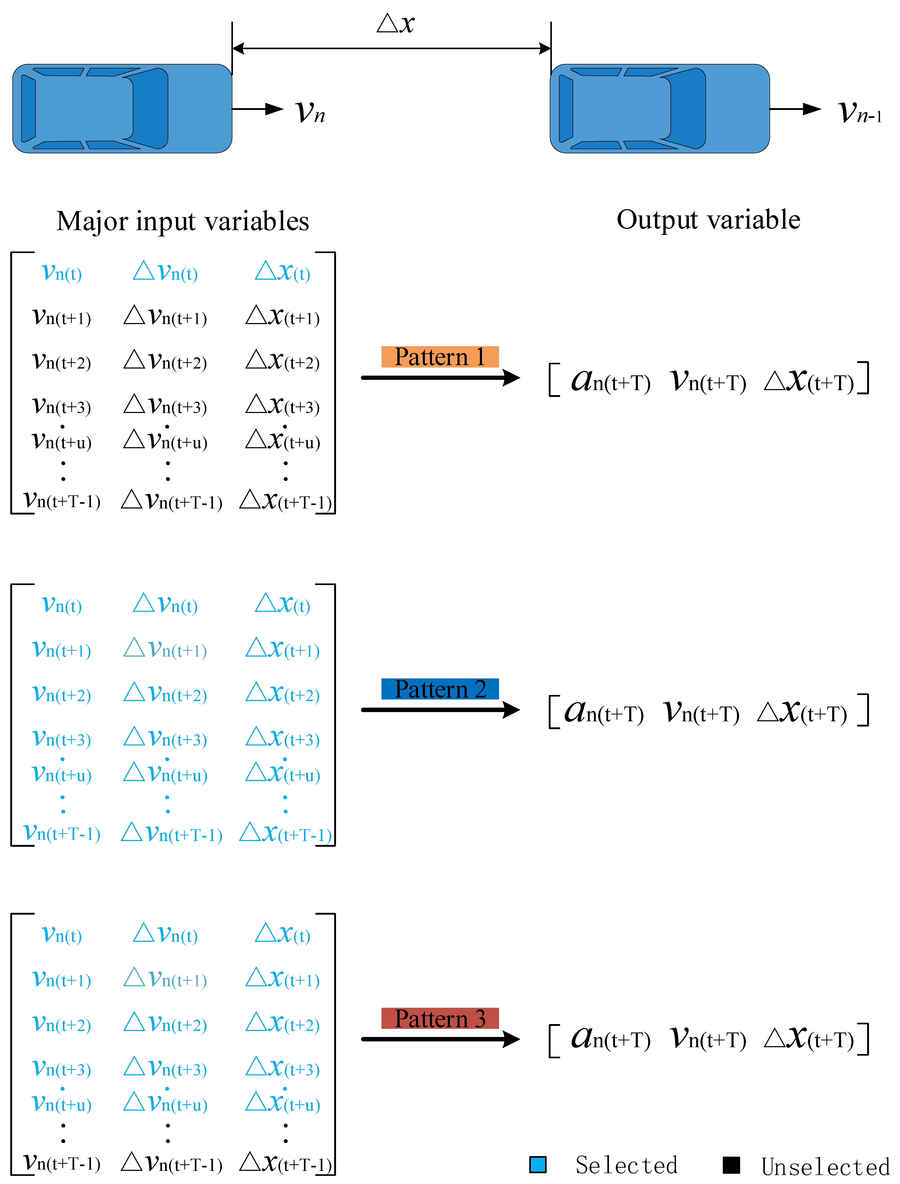
4. Method
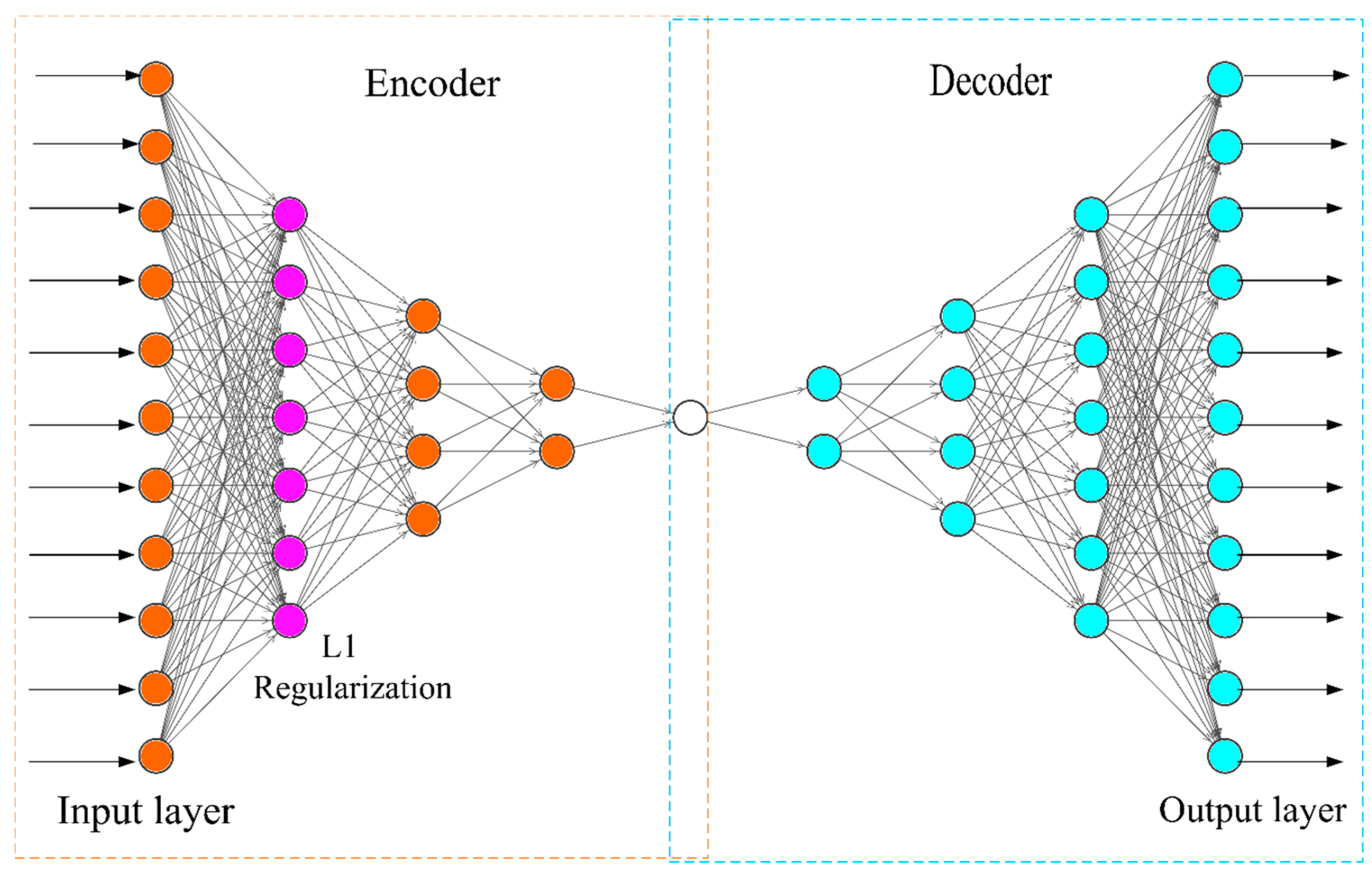
4.1. Extracting Features Using Autoencoder
4.2. Testing on NGSIM Datasets
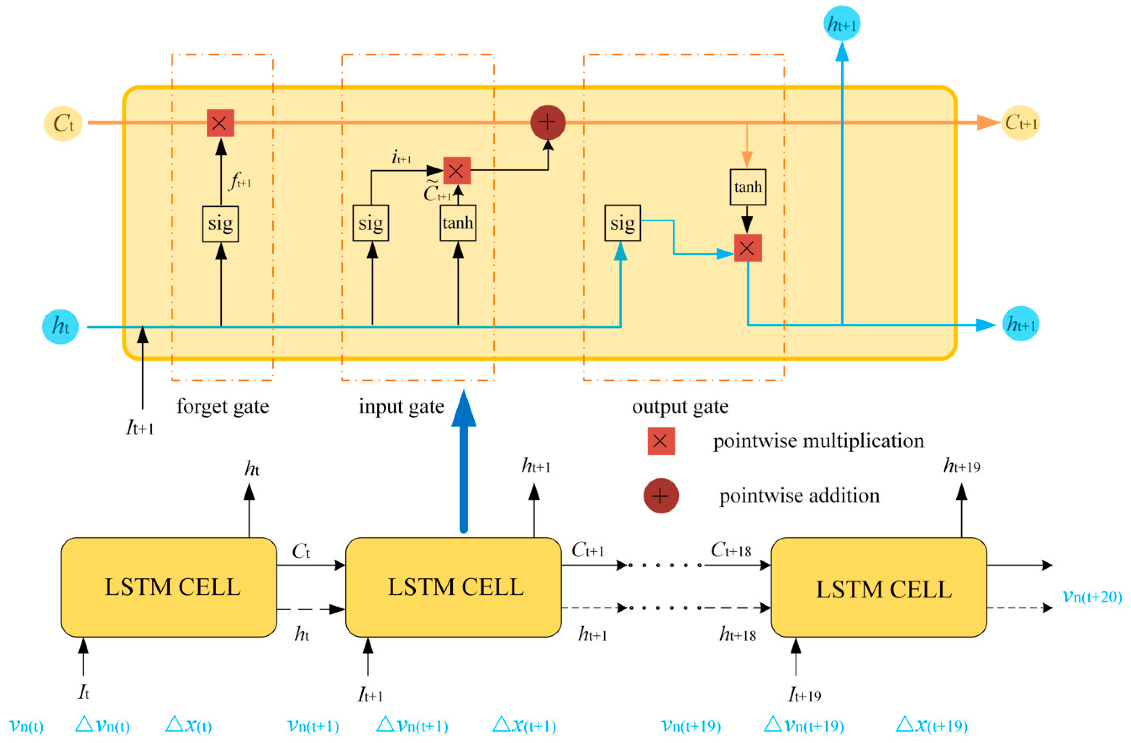
4.3. Car-Following Model Based on LSTM
4.3.1. Long Short-Term Memory Neural Network in CF Models
4.3.2. Model Setups for CF Modeling
5. Results
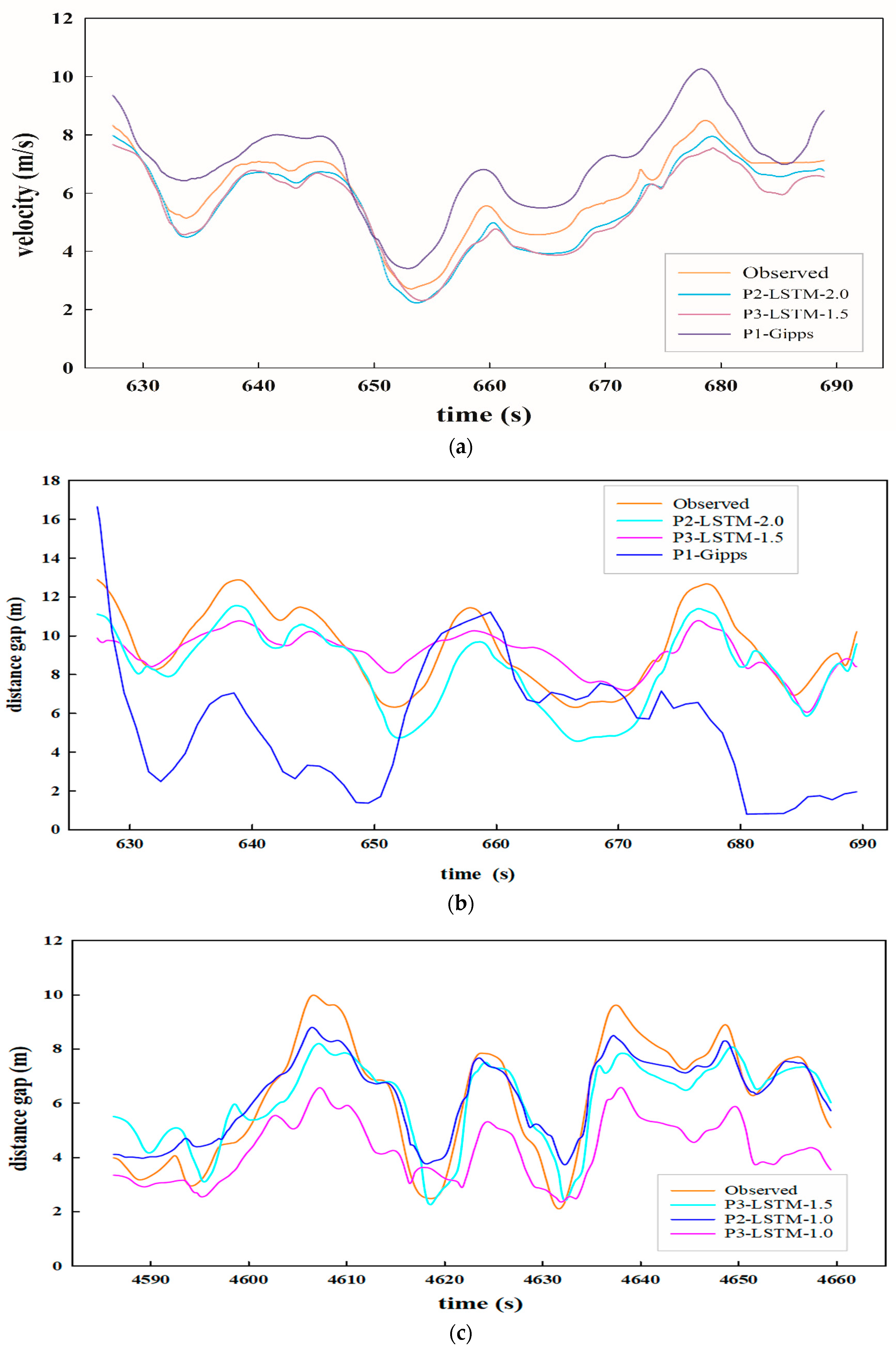
- The LSTM model can learn the driving memory information and describe car-following behaviors with high accuracy especially when using the prediction strategy of pattern 2, because of the LSTM’s unique structure and the incorporation of important temporal information. Figure 6c shows that when v, △v, t were used as inputs, the model did not perform as well in predicting the distance gap. The Gipps model showed acceptable performance in predicting the velocity gap but did not provide good indirect predictions of the distance gap, with estimates substantially lower than the observed value when v, △v, △x were used as inputs (see Figure 6b).
- The time gap parameter ranked highly in the autoencoder analysis, but did not lead to better results, because it is dependent on the velocity parameter. Taking both the time gap and velocity as inputs introduced redundant information and did not improve model performance. Therefore, the variable set of v, △v and △x is recommended instead.
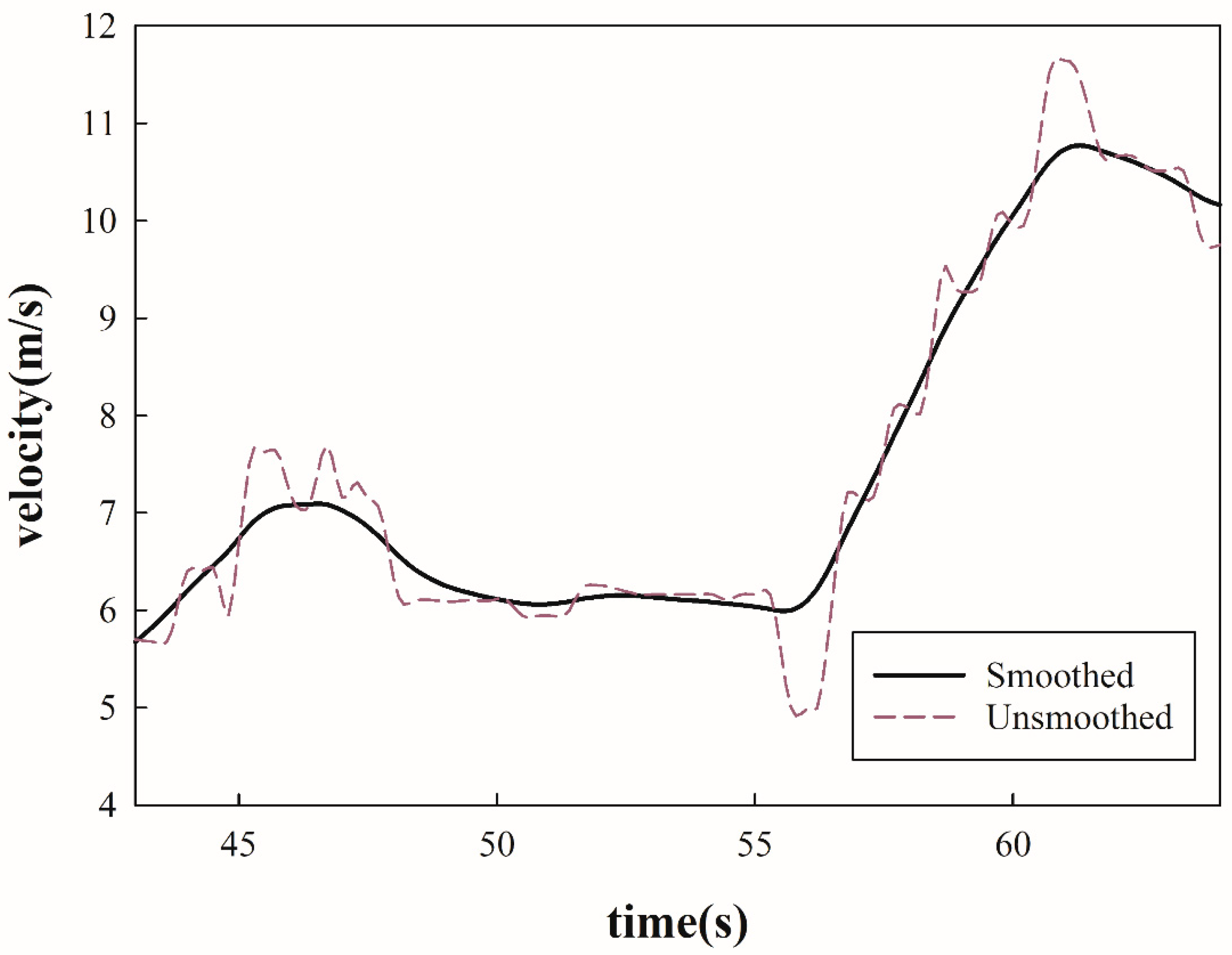
- In most cases, the model showed the best performance with 2.0 s as the time window in pattern 2. Only when predicting the distance gap, the model with a 1.0 s time window and with v, △v, △x as inputs performed better. The optimal time window for predicting velocity and distance gaps needs to be further investigated. A larger time window may lead to better performance, but will also lead to increased computational requirements, increased training time, and (potentially) convergence difficulty during training.
- For pattern 3, the reaction time and the historical driving memory were both considered explicitly, reflecting real driving behaviors. Some key temporal information has been removed, so the predictions are of slightly lower accuracy than using pattern 2 but are still acceptable (see Figure 6c, where v, △v, t are used as inputs). The model showed increased prediction error with 1.0 s time window as a considerable amount of key information was lost. Therefore, incorporating reaction time and historical driving memory at the same time remains challenging for car-following modeling.
- Results show that the prediction accuracy of the proposed LSTM model with patterns 2 and 3 was higher than that of existing models (i.e., the Gipps model).
6. Conclusions
Author Contributions
Funding
Conflicts of Interest
References
- WHO. Global Status Report on Road Safety 2018; World Health Organization: Geneva, Switzerland, 2018. [Google Scholar]
- Wang, J.; Zhang, L.; Lu, S.; Wang, Z. Developing a car-following model with consideration of driver’s behavior based on an Adaptive Neuro-Fuzzy Inference System. J. Intell. Fuzzy Syst. 2015, 30, 461–466. [Google Scholar] [CrossRef]
- Zhou, M.; Qu, X.; Li, X. A recurrent neural network based microscopic car following model to predict traffic oscillation. Transp. Res. Part C Emerg. Technol. 2017, 84, 245–264. [Google Scholar] [CrossRef]
- Jiang, R.; Wu, Q.; Zhu, Z. Full velocity difference model for a car-following theory. Phys. Rev. E 2001, 64, 017101. [Google Scholar] [CrossRef] [PubMed]
- Saifuzzaman, M.; Zheng, Z. Incorporating human-factors in car-following models: A review of recent developments and research needs. Transp. Res. Part C Emerg. Technol. 2014, 48, 379–403. [Google Scholar] [CrossRef]
- Schmidhuber, J. Deep learning in neural networks: An overview. Neural Netw. 2015, 61, 85–117. [Google Scholar] [CrossRef]
- Lee, G. A Generalization of Linear Car-Following Theory. Oper. Res. 1966, 14, 595–606. [Google Scholar] [CrossRef]
- Durrani, U.; Lee, C.; Maoh, H. Calibrating the Wiedemann’s vehicle-following model using mixed vehicle-pair interactions. Transp. Res. Part C Emerg. Technol. 2016, 67, 227–242. [Google Scholar] [CrossRef]
- Gipps, P. A behavioural car-following model for computer simulation. Transp. Res. Part B Methodol. 1981, 15, 105–111. [Google Scholar] [CrossRef]
- Newell, G. A simplified car-following theory: A lower order model. Transp. Res. Part B Methodol. 2002, 36, 195–205. [Google Scholar] [CrossRef]
- Khodayari, A.; Ghaffari, A.; Kazemi, R.; Braunstingl, R. A Modified Car-Following Model Based on a Neural Network Model of the Human Driver Effects. IEEE Trans. Syst. Man Cybern. Part A Syst. Hum. 2012, 42, 1440–1449. [Google Scholar] [CrossRef]
- Chong, L.; Abbas, M.M.; Medina, A. Simulation of Driver Behavior with Agent-Based Back-Propagation Neural Network. Transp. Res. Rec. J. Transp. Res. Board 2011, 2249, 44–51. [Google Scholar] [CrossRef]
- Wei, D.; Liu, H. Analysis of asymmetric driving behavior using a self-learning approach. Transp. Res. Part B Methodol. 2013, 47, 1–14. [Google Scholar] [CrossRef]
- Zhu, M.; Wang, X.; Wang, Y. Human-like autonomous car-following model with deep reinforcement learning. Transp. Res. Part C Emerg. Technol. 2018, 97, 348–368. [Google Scholar] [CrossRef]
- Huang, X.; Sun, J.; Sun, J. A car-following model considering asymmetric driving behavior based on long short-term memory neural networks. Transp. Res. Part C Emerg. Technol. 2018, 95, 346–362. [Google Scholar] [CrossRef]
- Wang, X.; Jiang, R.; Li, L.; Lin, Y.-L.; Wang, F.-Y. Long memory is important: A test study on deep-learning based car-following model. Phys. A Stat. Mech. Appl. 2019, 514, 786–795. [Google Scholar] [CrossRef]
- NGSIM: Next Generation Simulation. FHWA, U.S. Department of Transportation. Available online: www.ngsim.fhwa.dot.gov (accessed on 1 April 2019).
- Thiemann, C.; Treiber, M.; Kesting, A. Estimating Acceleration and Lane-Changing Dynamics from Next Generation Simulation Trajectory Data. Transp. Res. Rec. J. Transp. Res. Board 2008, 2088, 90–101. [Google Scholar] [CrossRef]
- Naseri, H.; Nahvi, A.; Karan, F.S.N. A new psychological methodology for modeling real-time car following maneuvers. Travel Behav. Soc. 2015, 2, 124–130. [Google Scholar] [CrossRef]
- Van Winsum, W. The human element in car following models. Transp. Res. Part F Traffic Psychol. Behav. 1999, 2, 207–211. [Google Scholar] [CrossRef]
- Zaky, A.B.; Gomaa, W. Car following regime taxonomy based on Markov switching. In Proceedings of the 17th International IEEE Conference on Intelligent Transportation Systems (ITSC), Qingdao, China, 8–11 October 2014; pp. 1329–1334. [Google Scholar]
- Ma, X.; Andreasson, I. Behavior Measurement, Analysis, and Regime Classification in Car Following. IEEE Trans. Intell. Transp. Syst. 2007, 8, 144–156. [Google Scholar] [CrossRef]
- Hosseini-Asl, E.; Zurada, J.M.; Nasraoui, O. Deep Learning of Part-based Representation of Data Using Sparse Autoencoders with Nonnegativity Constraints. IEEE Trans. Neural Netw. Learn. Syst. 2016, 27, 2486–2498. [Google Scholar] [CrossRef]
- Chen, J.; Wu, Z.; Zhang, J. Driver identification based on hidden feature extraction by using adaptive nonnegativity-constrained autoencoder. Appl. Soft Comput. 2019, 74, 1–9. [Google Scholar] [CrossRef]
- Guo, J.; Liu, Y.; Zhang, L.; Wang, Y. Driving Behaviour Style Study with a Hybrid Deep Learning Framework Based on GPS Data. Sustainability 2018, 10, 2351. [Google Scholar] [CrossRef]
- Liu, H.; Taniguchi, T.; Tanaka, Y.; Takenaka, K.; Bando, T. Visualization of Driving Behavior Based on Hidden Feature Extraction by Using Deep Learning. IEEE Trans. Intell. Transp. Syst. 2017, 18, 2477–2489. [Google Scholar] [CrossRef]
- Wiedemann, D. Simulation des Straßenverkehrsflusses; Schriftenreihe des Instituts für Verkehrswesen: Karlsruher, Germany, 1974. [Google Scholar]
- Raju, N.; Kumar, P.; Arkatkar, S.; Joshi, G. Determining risk-based safety thresholds through naturalistic driving patterns using trajectory data on intercity expressways. Saf. Sci. 2019, 119, 117–125. [Google Scholar] [CrossRef]
- Wang, F.; Dai, M.; Sun, L.; Jin, S. Mixed distribution model of vehicle headway based on multiclass car following. J. Zhejiang Univ. Eng. Sci. 2015, 49, 1288–1294. [Google Scholar]
- Chollet, F. Keras Document. Available online: https://keras.io (accessed on 15 April 2019).
- Zhang, X.; Bham, G.H. Estimation of driver reaction time from detailed vehicle trajectory data. In Proceedings of the 18th IASTED International Conference on Modelling and Simulation, Montreal, QC, Canada, 30 May–1 June 2007; pp. 574–579. [Google Scholar]
- Vasconcelos, L.; Neto, L.; Santos, S.; Silva, A.B.; Seco, Á. Calibration of the Gipps Car-following Model Using Trajectory Data. Transp. Res. Procedia 2014, 3, 952–961. [Google Scholar] [CrossRef] [Green Version]


| Symbols | Meaning | Upper Bound | Lower Bound | Unit |
|---|---|---|---|---|
| IPT | Instantaneous perception time | 18 | 0.3 | s |
| The average velocity during the time window | 22 | 0 | m/s | |
| The minimum velocity difference during the time window (negative) | 0 | −6 | m/s | |
| The maximal velocity difference during the time window (positive) | 6 | m/s | ||
| The maximal absolute value of all velocity difference values | 6 | 0 | m/s | |
| The minimum distance gap during the time window | 45 | 0.5 | ||
| The maximal distance gap during the time window | 45 | 0.5 | ||
| The average distance gap during the time window | 45 | 0.5 | ||
| The minimum time gap during the time window | 5 | 0.2 | s | |
| The maximal time gap during the time window | 5 | 0.2 | s | |
| The average time gap during the time window | 5 | 0.2 | s |
| Parameters | Value | Parameters | Value |
|---|---|---|---|
| Learning rate | 0.009 | Loss function | See Equation (4) |
| Epochs | 25 | Optimizer | Adam |
| Batch size | 40 | Number of hidden layers | 7 |
| Activation function | tanh | Sparsity penalty (α) | 0.002 |
| Parameter | Model Run 1 | Model Run 2 | Model Run 3 | Average Activation |
|---|---|---|---|---|
| 1.743 | 1.182 | 1.334 | 1.420 | |
| 1.491 | 1.147 | 1.087 | 1.242 | |
| 1.434 | 1.149 | 1.115 | 1.233 | |
| 1.365 | 1.162 | 1.051 | 1.193 | |
| 1.361 | 1.065 | 1.088 | 1.171 | |
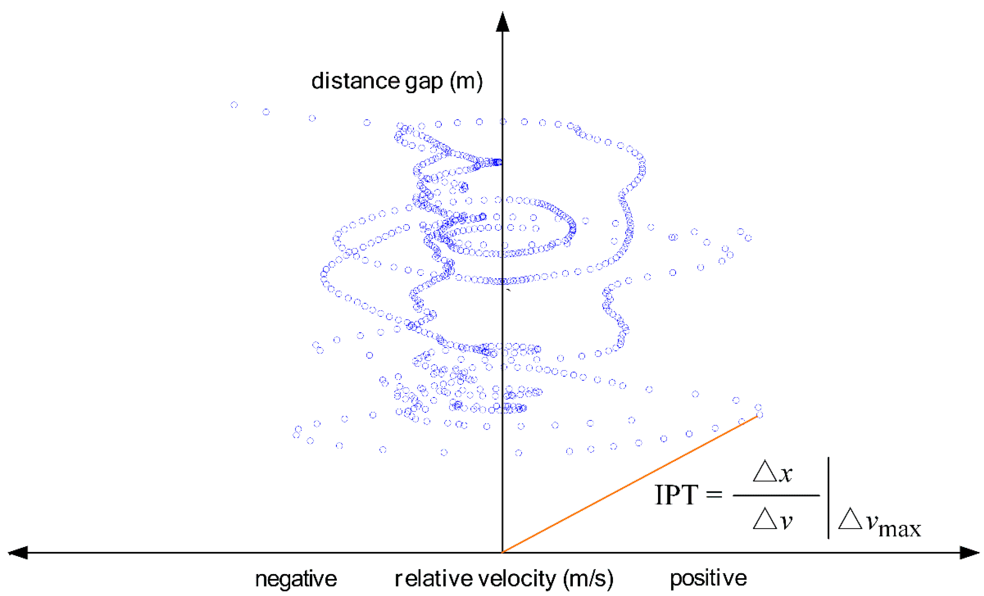
| IPT | 1.295 | 1.134 | 1.032 | 1.154 |
| 1.151 | 1.14 | 0.858 | 1.050 | |
| 0.979 | 1.152 | 0.759 | 0.963 | |
| 0.998 | 1.055 | 0.79 | 0.948 | |
| 0.715 | 0.751 | 0.571 | 0.679 | |
| 0.255 | 0.446 | 0.278 | 0.326 |
| Parameters | Value | Parameters | Value |
|---|---|---|---|
| Learning rate | 0.002 | Loss function | RMSE |
| Epoch | 2 | Optimizer | Adam |
| Number of LSTM cells | 60 | Batch size | ≥587 |
| Activation function | ReLU * | Time steps | 20/10 |
| Number of LSTM layers | 4 | Dropout rate | 0.2 |
| Pattern | Window Length (s) * | Input Variables | Output Variables | |||
|---|---|---|---|---|---|---|
| Velocity | Distance Gap | |||||
| MSE | MAPE (%) | MSE | MAPE (%) | |||
| 1 | 0.1 | 2.494 | 24.396 | − | − | |
| 2 | 2.0 | 0.264 | 6.951 | 3.285 | 16.555 | |
| 2 | 2.0 | 0.589 | 9.689 | 4.855 | 17.192 | |
| 2 | 1.0 | 0.367 | 9.045 | 1.705 | 11.467 | |
| 2 | 1.0 | 1.227 | 16.474 | 2.795 | 14.044 | |
| 3 | 1.0 | 0.986 | 12.942 | 3.065 | 15.076 | |
| 3 | 1.0 | 2.353 | 22.163 | 12.543 | 31.612 | |
| 3 | 1.5 | 0.624 | 10.364 | 4.178 | 16.762 | |
| 3 | 1.5 | 2.148 | 18.337 | 4.954 | 20.771 | |
© 2019 by the authors. Licensee MDPI, Basel, Switzerland. This article is an open access article distributed under the terms and conditions of the Creative Commons Attribution (CC BY) license (http://creativecommons.org/licenses/by/4.0/).
Share and Cite
Fan, P.; Guo, J.; Zhao, H.; Wijnands, J.S.; Wang, Y. Car-Following Modeling Incorporating Driving Memory Based on Autoencoder and Long Short-Term Memory Neural Networks. Sustainability 2019, 11, 6755. https://doi.org/10.3390/su11236755
Fan P, Guo J, Zhao H, Wijnands JS, Wang Y. Car-Following Modeling Incorporating Driving Memory Based on Autoencoder and Long Short-Term Memory Neural Networks. Sustainability. 2019; 11(23):6755. https://doi.org/10.3390/su11236755
Chicago/Turabian StyleFan, Pengcheng, Jingqiu Guo, Haifeng Zhao, Jasper S. Wijnands, and Yibing Wang. 2019. "Car-Following Modeling Incorporating Driving Memory Based on Autoencoder and Long Short-Term Memory Neural Networks" Sustainability 11, no. 23: 6755. https://doi.org/10.3390/su11236755
APA StyleFan, P., Guo, J., Zhao, H., Wijnands, J. S., & Wang, Y. (2019). Car-Following Modeling Incorporating Driving Memory Based on Autoencoder and Long Short-Term Memory Neural Networks. Sustainability, 11(23), 6755. https://doi.org/10.3390/su11236755