Article

Truck Arrivals Scheduling with Vessel Dependent Time Windows to Reduce Carbon Emissions

1
College of Transportation Engineering, Dalian Maritime University, Dalian 116026, China
2
Institute of Transportation Strategy Management and Systematic Planning, Dalian Maritime University, Dalian 116026, China
3
College of Transport and Communications, Shanghai Maritime University, Shanghai 201306, China
*
Author to whom correspondence should be addressed.
Sustainability 2019, 11(22), 6410; https://doi.org/10.3390/su11226410
Submission received: 12 October 2019 / Revised: 10 November 2019 / Accepted: 12 November 2019 / Published: 14 November 2019
(This article belongs to the Special Issue Sustainable Development of Seaports)

Abstract

:
Irregular external truck arrivals at a marine container terminal often leads to long queues at gates and substantial greenhouse gas emissions. To relieve gate congestion and reduce carbon emissions, a new truck arrival pattern called “vessel dependent time windows (VDTWs)” is proposed. A two-phase queuing model is established to describe the queuing process of trucks at gate and yard. An optimization model is established to assign time window and appointment quota for each vessel in a marine container terminal running a terminal appointment system (TAS) with VDTWs. The objective is to minimize the total carbon dioxide emissions of trucks and rubber-tired gantry cranes (RTGCs) during idling. The storage capacity constraints of each block and maximum queue length are also taken into consideration. A hybrid genetic algorithm based on simulated annealing is developed to solve the problem. Results based on numerical experiments demonstrate that this model can substantially reduce the waiting time of trucks at gate and yard and carbon dioxide emissions of trucks and RTGCs during idling.

1. Introduction

Maritime transport, as an economic and environmental friendly transport mode, is playing an increasingly important role in international trade [1]. The UNCTAD report revealed that more than 80% of world merchandise trade in terms of volume is transported by sea and handled at seaports [2]. Maritime transport has also been the backbone of the manufacturing supply chain [3]. According to the research conducted by Munim and Schramm, the quality of port infrastructure has a great effect on logistics performance and national economy [4]. However, daily production activities in seaports may consume a lot of energy and generate a large amount of greenhouse gas (GHG) emissions. The World Resources Institute reports that transportation accounts for approximately 15% of total global GHG emissions. The third IMO GHG study revealed that international shipping generates approximately 2.2% of global CO2 emissions [5]. Continuous rise of average temperatures due to CO2 emissions may result in disastrous consequences at a global level [6]. Climate change is one of the most urgent challenges faced by all regions in the world. Sustainable development of transportation has become a hot topic from both industrial and social perspectives. Governments and industries are under an increasing pressure to put forward more climate-friendly strategies. The Paris Climate Agreement (COP21) was adopted in December 2015 to reduce the emission of GHG. It was signed by 197 countries and ratified by 185 in January 2019. In August 2015, the Environmental Protection Agency (EPA), an independent agency of the United States’ federal government for environmental protection, announced the Clean Power Plan. Many European countries also adopted some national policies aimed at reducing emissions. Members-States adopted the 2030 EU Climate plan and Energy Package in October 2014. In June 2015, China submitted a document to the Intergovernmental Panel on Climate Change (IPCC) and became the 15th party to submit its own independent contribution. Port is an important logistic hub, but is also a major energy consumer. Therefore, reducing carbon emissions and energy consumption at port is crucial to achieve the climate goal [7]. The No. 94 document released by China in 2016 set a target of reducing carbon dioxide emissions and energy consumption per unit of port throughput by 2% in 2020, compared with 2015.
The emergence of the container has changed the method of freight transport through sea routes. Containerization has greatly improved port handling efficiency and lowered freight rates [8]. After the development of more than half a century, container liner shipping has become one of the most important transportation modes in international trade. Statista reported that approximately 60% of all world seaborne trade in terms of value is carried by container ships [9]. Nowadays, maritime container terminals have to face increasingly rough requirements by shipping companies which claim real-time services [10]. In order to be selected as hub ports or origin-destination points in shipping routes, marine container terminals have to improve their management capabilities and productivity [11,12,13]. In marine container terminals, handling operations can be divided into three types: Vessel operations, receiving/delivery operations by trucks, container handling and storage operations in the terminal yard. During the receiving operation, an outbound container arrives at the marine container terminal via an external truck and is inspected at the gate, and the stored location for this outbound container is informed to the truck driver. Then the external truck arrives at the transfer point, a yard crane receives the container from the truck [14]. The process of delivery operation is carried out in an opposite direction. The external trucks and yard cranes are the main contributors of GHG emission during the receiving/delivery operations. Global container throughput is generally growing. Furthermore, many liner shipping companies continue to increase the scale of deep-sea container vessels, as larger vessels can lower voyage costs per container due to economies of scale. The carrying capacity of container ships has increased significantly over the last 50 years [15]. Generally, the external trucks arrive at the marine container terminal randomly and nonuniformly, which leads to a large number of trucks get in and out of the terminal during peak hours. Truck arrivals exceeding the capacity of gate and yard can lead to heavy congestion. Long truck queues directly affect the operational efficiency of terminals. Meanwhile, truck and yard cranes idling due to congestion may lead to more fuel consumption and carbon dioxide emissions. Therefore, how to decrease the length of truck queues and increase handling efficiency of yard cranes in the terminal considering energy consumption is an important issue for the terminal operator, truck fleet, and government regulators. In recent years, marine container terminals have adopted some measures to alleviate congestion. According to the conceptual framework of queuing theory, these congestion alleviation measures can be classified into three categories. The first category of measures increases the number of gate lanes and yard cranes, or extends working hours at the gate. The second category of measures controls the truck arrival rate by truck arrival management (TAM). The third category of measures improve gate service rate by introducing an IT system [16]. Owing to the scarcity of port land, shoreline resources, and construction funds, it can be very difficult for marine container terminals to expand. Moreover, the required investments of purchasing yard cranes are generally very large. Furthermore, China’s marine container terminals already work in a 24/7 schedule. Therefore, the second category of congestion control measures are relatively effective approaches to solve the congestion problem and have been commonly used. TAM, mainly including tariff/toll pricing policies (TTPP), a terminal appointment system (TAS), and vessel dependent time windows (VDTWs), has received much attention. The TTPP motivates truckers to shift their arrival times by charging a higher traffic mitigation fee (or toll fee) for trucks entering the marine container terminal during peak hours. The TAS was first introduced in the Vancouver port of Canada, and many marine container terminals in North America followed. At present, the ports of Los Angeles and Long Beach in America [17] and Tianjin port in China have implemented TAS. By assigning hourly entry quotas and the maximum amount of trucks that can be accepted per time window, the TAS can reduce truck arrivals in peak periods, alleviate congestion, and improve operation efficiency at the marine container terminal. In addition, a reasonable yard working plan can be made to enhance the utilization rate of yard cranes. After these, both truck fleet and terminal operator can benefit from TAS. VDTWs assign time windows to each vessel, and trucks delivering/picking-up containers for/from the same vessel share one time window.
All these TAM measures are capable of alleviating congestion. However, both TTPP and TAS ignore the relationship between truck arrivals and vessel arrivals. The truck traffic flows in a marine container terminal are triggered by vessel arrival. The outbound/inbound containers for/from the same vessel are centrally allocated to some certain allowable blocks according to the well determined storage space allocation plan. Therefore, the distribution of trucks in each block is not uniform after entering the terminal gate. If the appointment quota is not related to a certain vessel, it is impossible to accurately calculate the truck arrivals in each block. The truck arrivals are also uncontrollable and it is difficult to effectively solve the congestion problem in the container terminal yard. In this paper, we try to fill this gap by combining TAS with VDTWs. At the same time, other constraints that exist in practical application are considered, including the storage space of each block and the maximum queue length. As a significant contributor of GHG emissions, the marine container terminals have responsibilities for energy saving and emission reduction. Therefore, this paper considers not only trucks waiting time but also CO2 emissions produced by idling trucks and rubber-tired gantry cranes (RTGCs).
The remainder of this paper is organized as follows. In Section 2, a literature review of terminal congestion alleviation is provided. Problem description and an optimization model for container delivery are given in Section 3. A hybrid genetic algorithm based on simulated annealing is developed to solve the problem in Section 4. Section 5 presents the results from numerical experiments. Conclusions are provided in Section 6.

2. Literature Review

A number of studies propose approaches to solve terminal congestion. These approaches can be classified into four types: Publishing terminal congestion information, TTPP, VDTWs, and the TAS. Mani and Fischer [18] proposed the methods of charging in peak periods and extending working hours to reduce peak-period congestion based on the Ports of Long Beach and Los Angeles, and indicated the implementation of TAS can improve the operation efficiency of terminal through relative analysis. Zeng et al. [19] considered the game-theoretical relationship between terminal operators, truckers, and government regulators and developed a bi-level programming model to determine the optimal congestion toll rates. Regarding terminal congestion information publication, Sharif et al. [20] studied the effect of terminal congestion information on the decision of truck drivers, and a simulation model is developed to simulate the decision-making process of truck drivers, which demonstrates that terminal congestion information can contribute to reducing the average turn time of trucks at the marine container terminal.
For VDTWs, Chen et al. [21] estimated the queue length at the gate based on a truck arrival pattern in each time window and optimized the time window of each vessel by using the non-stationary queuing theory to minimize the truck-side cost and the terminal-side cost. Wei [22] constructed a function of subsidies to terminal operators and a function of rehandling cost to truck fleet operators, and optimized the pickup time window based on the distribution of pickup times to reduce the rehandling operation. Chen and Jiang [23] systematically discussed the practical application of three alternative time windows optimized strategies, including fixed ending-point strategy (FEP), variable end-point strategy, and greedy algorithm strategy. Guo et al. [24] put forward an optimization model for vessel dependent truck appointment considering the total waste cost of truck fleet and yard cranes.
Some studies focused on the performance of TAS. In this respect, Morais and Lord [25] found that truck appointment can effectively alleviate port congestion, reduce the engine idling cost of trucks and the emissions of GHG, and improve operating efficiency based on TAS of the Canadian port. Huynh and Walton [26] simulated the operation process of trucks in container terminal yards to obtain the average turn time of trucks, then a mathematical formulation is applied to appoint truck number, which indicates that TAS can reduce the average turn time and improve the utilization of yard cranes. Namboothiri and Erera [27] studied the potential impact of the appointment system on drayage fleet efficiency, and a drayage operation plan is developed based on a port access control system to minimize transportation cost.
Moreover, some studies analyzed truck queuing behavior based on queuing theory and focused on the design and implementation of TAS. For example, Kim and Kim [28] found that the arrival process of outside trucks follows Poisson process and the service time of transfers is independent of each other, so the transfer operation can be formulated by the M/G/1 queuing model. Guan and Liu [29] took gate operating cost and the trucker’s cost associated with excessive waiting time into account, and a stationary M/Ek/C queuing model is applied to calculate the queue length at gate and optimize the appointment quota of different periods. However, due to the changing of truck arrivals and terminal service ability over time, it is not accurate to use stationary queuing models to estimate queue length. To fix this problem, Chen et al. [8] proposed a point-wise stationary approximation model to analyze time-dependent truck queuing processes at gate lanes and yard zones viewed as M/M/1 and M/G/1 queues, respectively, and a two phase optimization approach is used to compute a system optimal truck arrival pattern and a desirable pattern of time-varying tolls. Zeng [30] and Zhang [31] developed an optimization model for truck appointment to optimize the appointment quota based on the BCMP queuing network, and the M/Ek/C queuing model is applied to describe the queuing process of trucks at gate lanes and yard zones. Xu et al. [32] used queue theory and the stationary backlog-carryover approach to build the two-phase multi-objective queuing model at gate and yard, which can deal with the case when truck arrival rate exceeds gate service rate. Zhang et al. [33] proposed an optimization model of truck appointment considering coordinated service of inner and outer container trucks based on the vacation queuing system. Jiang et al. [34] optimized the appointment quota of different periods for each vessel according to the shipping schedule and the number of export containers. However, the yard crane scheduling generally affects the queuing model of the terminal yard and the waiting time of trucks in the terminal yard. Therefore, Yang et al. [35] proposed a new mechanism of appointment considering dynamic deployment of yard crane based on the two-way transmission of information between truck drivers and the marine container terminal. Ma et al. [36] developed a bi-level programming model integrating truck appointment and crane deployment.
From the above literature review, we find that existing researches on the measures to alleviate truck queuing mostly focused on the performance, design, and implementation of TAS. Most studies divide the decision period into several sub-periods and determine the appointment quota of each period, and truckers can choose their preferred appointment period. It can provide more choices for truckers. However, if the arrival time distribution of trucks that deliver containers for the same vessel is too scattered, it will affect the organizational efficiency of yard operation. In addition, the appointment optimization models in current literature paid little attention to the relationship between truck arrivals and vessel arrivals. Although the model proposed by Jiang [34] can determine the appointment quota of different periods for each vessel, the ratio of export containers of the same vessel stored at each certain block has not been considered. Because of this, the truck arrivals are still uncontrollable and it is difficult to effectively solve the congestion problem in a container terminal yard. In addition, the storage capacity of each block is limited. Obviously, existing appointment optimization models do not take this situation into account.
As a significant contributor of GHG emissions, marine container terminals have responsibilities for energy saving and emission reduction. A number of researches have investigated carbon emissions generated from various activities related to seaports. Carbon emissions are typically generated from container ships, equipments that are used to load, unload, and transport containers in the marine container terminal, and external trucks transporting containers between the marine container terminal and its hinterland. Some studies investigated generated air emissions during a container vessel’s maneuver and berth process. Goldsworthy [37] analyzed the impact of ship type, ship size, operating mode, and machinery type on air emissions in ports. Some studies calculated various emissions, air pollutants (NOx, PM10, SO2), and greenhouse gases (GHGs; CO2, CH4, N2O) of ships in different ports [38,39]. Some studies analyzed the air emissions generated from the equipment used in port operation. Yu et al. [40] evaluated the emissions from two states of yard tractors during loading, i.e., moving at normal speed and suffering from congestion. Liu and Ge [41] optimized the number of QCs in order to minimize emission from QCs and AGVs at idling state in queue during an unloading process of containers from QCs to AGVs. The Inventory of Air Emissions 2018 by POLA revealed that RTGCs accounted for approximately 10% of total CO2 emissions generated from cargo handling equipment in the terminal [42]. The RTGCs are sometimes in idling situation, waiting without work, during operation. Therefore, Li [43] introduced a reforming plan of RTGs’ engine with double speed unit to meet the need of continuous power supply and energy conservation. Yang and Chang [44] compared the performance of rubber-tired gantry cranes (RTGCs) and electric rubber-tired gantry cranes (E-RTGCs) from the perspective of energy savings and CO2 reduction. External trucks also contributed a large amount of air emissions during receiving/delivery operations from hinterland to port [45,46]. However, these studies only consider the air emissions of 1–2 operation processes related to vessels. Sim [47] used a system dynamics approach to calculate the total amount of carbon emissions produced during the entire processes in a container terminal related to a vessel. Previous studies only focused on truck idling emissions and did not take yard crane idling emissions into account.
In this study, we try to fill these gaps by proposing a new terminal appointment system with VDTWs, which designates a truck arrival time window for each vessel, divides the time window into several appointment periods, and determines the appointment quota of each period for each vessel to minimize the total carbon dioxide emissions of truck fleet and RTGCs. This paper makes the following main contributions: (1) It combines TAS with VDTWs, which can make truck arrivals at the terminal yard more controllable; (2) it considers the storage of export containers from the same vessel in different blocks, so that it can be guaranteed that the storage capacity limit is not exceeded under an optimized truck arrival pattern; (3) as a yard system is typically a bottleneck, this paper considers the constraint of the maximum queue length, so as to effectively control the congestion in the terminal yard; (4) considering the external trucks and RTGCs are both contributors of GHG emission during the receiving/delivery operations, this paper aims to reduce CO2 emissions produced by idling trucks and RTGCs.

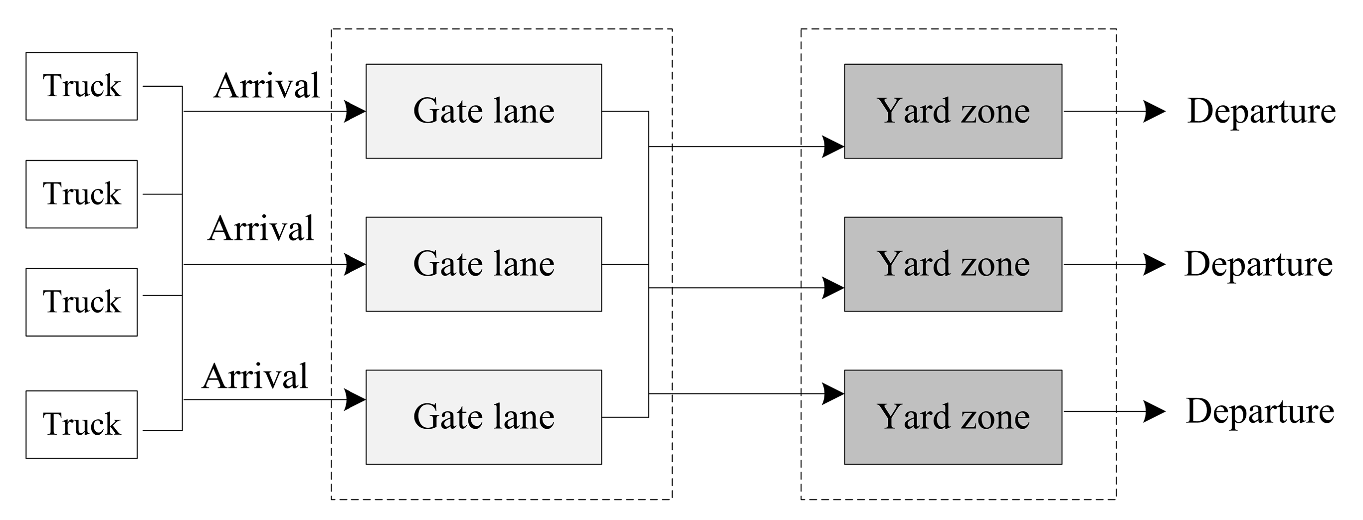
3. Problem Description

Determining the truck arrival time window for each vessel and the appointment quota of each period is the key to the implementation of TAS. The truck arrival time window for each vessel consists of the starting point and ending point of the time window. Each time window is equally divided into several appointment periods, and the appointment quota is the maximum amount of trucks of each appointment period. In this paper, the proposed a truck arrival pattern based on VDTWs establishing an effective connection between the terminal and the outside yard. For each vessel calling at the terminal, the terminal firstly releases the time window and determines the appointment quota of each period. Next, the outside yards choose the appropriate appointment period and make an appointment for export drop-offs according to their transport capacity. Then, the terminal confirms the final truck arrival planning and informs each yard, and yards arrange trucks to deliver containers. The process of truck entering the port is as follows: A truck picks up containers in the outside yard and delivers containers to the port, and it has to wait for entering the port when the gate is busy; then, the truck arrives at the predetermined block waiting for the unloading operation of RTGC after the gate checks containers and prints the admission ticket; the truck leaves the yard with containers unloaded, and then leaves the gate after finishing the departure formalities. Therefore, a two-phase queuing system is developed to describe the queuing process of trucks at gate and yard, as is shown in Figure 1.
The number of hourly truck arrivals in one week is shown in Figure 2. It can be seen that the arrival pattern of the delivery trucks is obviously uneven. That is to say, the arrival rate of the delivery trucks varies with time. Therefore, some studies assume that the arrival of the delivery trucks is a non-homogeneous Poisson process (NHPP) [8,31,48]. It is important to apply statistical tests to determine if an NHPP is actually appropriate for the arrival pattern of the delivery trucks. To solve this problem, Brown et al. [49,50] converted it into a standard statistical test to determine whether data can be regarded as a sample from a sequence of independent and identically distributed random variables with a specified distribution. Because of the continuous and slow change of the arrival rate with time, NHPP can be transformed into a piecewise-constant non-homogeneous Poisson process (PC NHPP). Thus, the arrival rate of the delivery trucks is constant in a sufficiently short interval. Therefore, the NHPP test can be divided into two steps. The first step is to divide a day into several short intervals, so that the arrival rate of the delivery trucks in each interval does not change significantly. The second step is to test whether the arrival of the delivery trucks is homogeneous in the subset of these short intervals. For example, the intervals at the same time of multiple days or multiple continuous intervals in a day. The commonly used NHPP statistical test models are: CU KS test and Log KS test.
(1)
CU KS test
One day is divided into B short intervals, n b delivery trucks arrive at the marine container terminal within the b th ( b = 1 , 2 , , B ) interval [ 0 , L ] . Let T a b denote the arrival time of the a th delivery trucks arriving at the marine container terminal within the b th interval, T 1 b T 2 b T n b b . Applying the CU transformation to transform random variable T a b into random variable U a b = T a b / L , { U a b } U ( 0 , 1 ) . The KS test is based on the maximum difference between the empirical cumulative distribution function F n b ( x ) and underlying cumulative distribution function F ( x ) [50]:
D n b = m a x x { | F n b ( x ) F ( x ) | } ,
F n b ( x ) = 1 n b a = 1 n b I ( U a b x ) 0 x 1 ,
F ( x ) = x 0 x 1 ,
where I ( · ) is the indicator function.
(2)
Log KS test
Brown [49,50] constructed an exponential random variable R a b with parameter 1 through the log transformation.
R a b = ( n b + 1 a ) ( l o g ( L T a b L T a 1 , b ) ) a = 1 , 2 , n b
F n b ( x ) = 1 n b a = 1 n b I ( R a b x ) 0 x 1
F ( x ) = 1 e x
Kim et al. [50] indicated that the sample size of each subset about 200–300 is sufficient and reasonable. Therefore, the short intervals are set, according to Table 1, to reach the sample size. We set L = 1 h and L = 0.5 h, respectively, the test results of CU KS test and Log KS test are shown in Table 1. We compare the p-value of the test to the significance level α = 0.05 . If the p-value is less than 0.05, we reject the null hypothesis that the arrival of the delivery trucks is a non-homogeneous Poisson process. For L = 1 h, only 27 subsets’ p-values of the CU KS test are greater than 0.05, and 24 subsets’ p-values of the Log KS test are greater than 0.05. However, when we set L = 0.5 h, 40 subsets’ p-values of the CU KS test are greater than 0.05, and 31 subsets’ p-values of the Log KS test are greater than 0.05. These four subsets that fail to pass the CU KS test pass the Log KS test. Moreover, on the whole, E ( P C U ) = 0.3631 and E ( P L o g ) = 0.1908 . The results show that the arrival of the delivery trucks is a non-homogeneous Poisson process.
The service time of the terminal gate during six consecutive hours is counted, and the frequency distribution histogram is shown in Figure 3. The Chi-square goodness of fit test is a most commonly used technique for testing whether a sample of data comes from a population with a specific distribution. The Chi-square statistic is defined as:
χ 2 = i = 1 k ( N i e i ) 2 e i ,
e i = n [ F ^ ( C i ) F ^ ( C i 1 ) ] ,
where N i represents the observed frequency in category i; e i represents the expected frequency in category i; [ C i 1 , C i ) represents the range of category i; F ^ ( x ) represents the cumulative distribution function of terminal gate service time.
Under the null hypothesis that the terminal gate service time follows the exponential distribution, the critical value at the 0.05 significance level is 18.31. According to formula (7) and (8), we calculated the Chi-square statistic χ 2 = 17.778 . Chi-square statistic is less than the critical value, therefore, we do not reject the hypothesis that the service time of the terminal gate follows the exponential distribution. The gate lanes with single waiting lines can be viewed as multiple independent M(t)/M/1.
According to Burke’s theorem, the M/M/1 queuing system in the stationary state has a departure process identical to the arrival process, so the departure process of customers is viewed as a Poisson process and the discharge rate is equal to the arrival rate [51]. Therefore, the arrival process of trucks to yard zone can be regarded as a Poisson process. The service time of the RTGCs during six consecutive hours is counted, and the frequency distribution histogram is shown in Figure 4. Under the null hypothesis that the service time of RTGCs follows the exponential distribution, the critical value at the 0.05 significance level is 37.68. According to formula (7) and (8), we calculated the Chi-square statistic χ 2 = 602.947 . Chi-square statistic is larger than the critical value, therefore, we reject the hypothesis that the service time of RTGCs follows the exponential distribution. Under the null hypothesis that the service time of RTGCs follows the Erlang distribution, the critical value at the 0.05 significance level is 36.42. According to formula (7) and (8), we calculated the Chi-square statistic χ 2 = 139.2506 . Chi-square statistic is larger than the critical value, therefore, we reject the hypothesis that the service time of RTGCs follows the Erlang distribution. Furthermore, the service time of the RTGCs can be easily affected by the operating habits of the operators, the stacking rules of the export containers, and other factors. Therefore, it is assumed that the service time of the RTGCs follows the general distribution. The yard blocks can be viewed as multiple independent M(t)/G/K.
Since truck arrivals change over time, the queuing process of trucks at the gate and yard are non-homogeneous Poisson processes. A point wise stationary fluid flow approximation (PSFFA) [52,53] approach is applied to convert the non-homogeneous process into a sequence of time intervals, so that stationary approximations can be used to calculate the queuing length, while the arrival rate of delivery trucks at each yard block is different. In order to reasonably appoint the delivery of trucks, it is necessary to consider the limitation of yard capacity and queue length of each yard block.

4. Truck Appointment Model for Container Delivery

4.1. Model Assumptions

The following assumptions are used in the model:
  • Container vessels provide weekly liner service, so the planning period is one week;
  • The service capacity of each gate lane is the same, and the service capacity of each RTGC is the same;
  • The export containers on each vessel are centralized stores at several designated blocks in a certain proportion;
  • The gate lanes for delivery trucks and pickup trucks are set separately. Moreover, the export containers and import containers are stored at different blocks. Therefore, the influence of pickup trucks on delivery trucks is not considered;
  • Each block deploys K RTGCs, which only serve outside delivery trucks without inside trucks. RTGCs scheduling between different blocks is not considered. Since there will be containers arriving at the port on each vessel in each period, RTGCs have no time to serve other blocks with higher utilization rate;
  • In the gate layer, the gate lanes with single waiting lines can be viewed as multiple independent M(t)/M/1 queuing processes. In the yard layer, the yard blocks can be viewed as multiple independent M(t)/G/K queuing processes;
  • The ending point of the truck arrival time window for each vessel has to be earlier than the corresponding vessel arrival time so that the terminal has enough time to arrange shipment;
  • Considering the capacity limitation of the yard, when the queue length of trucks at a yard block reaches the upper limit, the delivery trucks are not allowed to enter the gate.

4.2. Variable Definitions

In this model, all the input variables, derived variables, and decision variables are listed.
Input variables:
  • z : Index of vessel, z = 1 , 2 , , Z , where Z is the number of vessels;
  • T z A : The estimated time of arrival of vessel z (h);
  • T z D : The estimated time of departure of vessel z (h);
  • V z : The volume of export containers related to vessel z (natural container);
  • c o : The CO2 emission factor of a delivery truck per hour while idling (kg/h);
  • c R : The CO2 emission factor of a RTGC per hour while idling (kg/h);
  • N: Planning horizon (day);
  • p: Index of appointment periods, where the planning horizon is divided into P periods, p = 1 , 2 , , P ;
  • t: Index of fluid-based modeling time intervals, where the planning horizon is divided into T time intervals t = 1 , 2 , , T ;
  • α : The average loading rate of delivery trucks;
  • i: Index of gate lane, i = 1 , 2 , , I , where I is the number of gate lanes;
  • j: Index of yard block, j = 1 , 2 , , J , where J is the number of yard blocks;
  • k : Index of RTGC deployed to one block, k = 1 , 2 , , K ;
  • β z j : The ratio of export containers of vessel z stored at block j;
  • Z j : The set of vessels whose export container are stored at block j;
  • u i t g : The service rate of gate lanes i at interval t (truck/h);
  • u j k t y : The service rate of the RTGC k deployed to block j at interval t (natural container/h);
  • C s : The coefficient of variation of service time distribution of a RTGC;
  • T l : The minimum length of time window for export containers on an arriving vessel;
  • T k : The maximum length of time window for export containers on an arriving vessel;
  • Y j : The maximum storage capacity of block j;
  • γ : The maximum of containers waiting in the queue at each block.
Derived variables:
  • m : The number of time intervals included in one appointment period;
  • λ z p : The appointment quota of export containers related to vessel z (arriving at terminal gate) at appointment period p;
  • λ z t g : The number of trucks related to vessel z arriving at terminal gate at interval t;
  • λ i t g : The number of trucks arriving at gate lane i at interval t;
  • l i t g : The average number of trucks waiting in queue at gate lane i at interval t;
  • d i t g : The actual discharge rate of gate lane i at interval t (truck/min);
  • ρ i t g : The capacity utilization rate of gate lane i at interval t;
  • w p g : The average waiting time of trucks at terminal gate during appointment period p (min);
  • w g : The average waiting time of trucks at terminal gate during the planning horizon (min);
  • λ t y : The number of export containers arriving at yard at interval t;
  • λ j t y : The number of export containers arriving at block j at interval t;
  • l j t y : The number of export containers waiting at block j at interval t;
  • d j k t y : The discharge rate of RTGC k deployed to block j at interval t (natural container/min);
  • ρ j k t y : The average utilization rate of RTGC k deployed to block j at interval t;
  • w j p y : The average waiting time of trucks at block j in appointment period p (min);
  • w y : The average waiting time of trucks at yard in the planning horizon (min);
  • d z p : d z p = 1 , if vessel z has departed at appointment period p; d z p = 0 , if vessel z is berthing in the marine container terminal at appointment period p.
Decision variables:
  • P z S : The starting appointment period for delivery trucks related to vessel z;
  • P z E : The ending appointment period for delivery trucks related to vessel z.

4.3. Optimization Model

4.3.1. Objective Function

The objective function (9) is to minimize the total CO2 emissions of truck fleet and RTGCs during idling. The first summation in the objective function corresponds to the CO2 emissions of truck fleet while waiting in line at the terminal gate and yard. The CO2 emissions of truck fleet during idling are calculated by multiplying the total waiting time at the terminal gate and yard by the CO2 emission factor of a delivery truck per hour during idling. The second summation describes the CO2 emissions of RTGCs during idling. RTGCs may wait without work during operation. The CO2 emissions of RTGCs during idling are calculated by multiplying the total idling time of all RTGCs by the CO2 emission factor of a RTGC per hour during idling.
m i n [ ( t = 1 T l t g + t = 1 T j = 1 J l j t y ) 24 N T c o + t = 1 T k = 1 K j = 1 J ( 1 ρ j k t y ) 24 N T c R ]

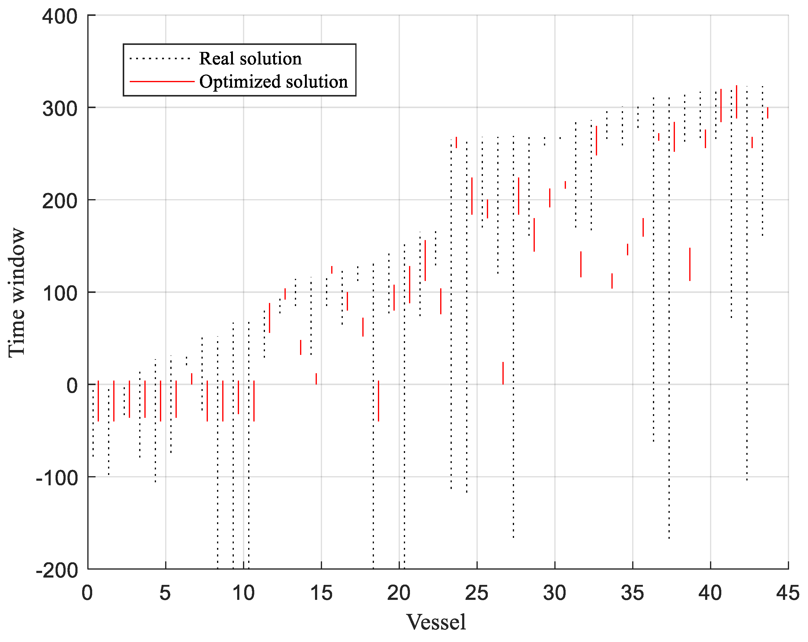
4.3.2. Time Window Optimization

Each vessel calling at the marine container terminal is assigned a truck arrival time window. Constraints (10) and (11) indicate that the length of time window for export containers on a delivering vessel must be longer than T l h and shorter than T k h. As a practical requirement of ship loading operation, constraint (12) requires that the ending point of a time window for export containers on each vessel has to be earlier than the estimated time of arrival of the corresponding vessel. Constraint (13) calculates the number of containers related to vessel z arriving at the terminal gate at appointment period p. Constraint (14) judges whether the vessel z has left the port during the appointment period p. Constraint (15) states the number of export containers arriving at each block should meet the storage capacity constraints of each block during the appointment period. After all the export containers related to vessel z have been loaded on board and vessel z departed the container terminal, the occupied stacking space can be released. Constraint (16) ensures that the starting and ending appointment period for delivery trucks related to vessel z are integer.
( p z E p z S + 1 ) 24 N P T l z
( p z E p z S + 1 ) 24 N P T k z
p z E 24 N P T z A z
λ z p = V z ( p z E p z S + 1 ) z , p
d z p = { 1   ,   ( p 1 ) 24 N P T z D 0   ,   ( p 1 ) 24 N P < T z D z , p
z Z j ( p = 1 p λ z p V z d z p ) β z j Y j j , p
p z E , p z S   is   integer

4.3.3. Constraints at Gate

The gate follows the FCFS principle, and the gate system can be described in a multiple server M(t)/M/1 queuing process. Constraint (17) calculates the number of time intervals included in one appointment period. As required by PSFFA, truck arrivals during appointment period p are converted into a sequence of arrivals for each interval. The number of trucks related to vessel z arriving at gate during interval t can be calculated with constraint (18). The aggregated truck arrivals are evenly distributes among gate lanes. Constraint (19) calculates the number of trucks arriving at gate lane i at interval t. Constraint (20) is the flow balance function based on the fluid-based approximation approach, which means that changes in the queue length at gate are equal to arrivals minus departures. Constraint (21) calculates the discharge rate of trucks at gate lane i at interval t. Constraint (22) indicates the relationship between the queue length at gate lane and the utilization rate of gate lane. Constraint (23) estimates the average waiting time of trucks at gate in appointment period p. Constraint (24) estimates the average waiting time of trucks at gate in the planning horizon.
m = T P
λ z t g = λ z p m α z , t = ( p 1 ) m + 1 , ( p 1 ) m + 2 , , p m
λ i t g = z = 1 Z λ z t g / I i , t
l i ( t + 1 ) g = max ( l i t g + λ i t g 24 · 60 N T d i t g , 0 ) i , t
d i t g = u i t g 60 ρ i t g i , t
l i t g = ρ i t g 1 ρ i t g i , t
w p g = t = ( p 1 ) m + 1 p m i = 1 I l i t g / t = ( p 1 ) m + 1 p m i = 1 I d i t g p
w g = t = 1 T i = 1 I l i t g / t = 1 T i = 1 I d i t g

4.3.4. Constraints at Yard

The yard system can be described in a multiple server M(t)/G/K queuing process. Constraint (25) calculates the number of trucks arriving at yard at interval t, which are determined by discharge rates of all the gate lanes. Constraint (26) calculates the number of export containers arriving at block j at interval t, which are determined by the number of trucks arriving at yard at interval t and a predefined yard destination proportion. Constraint (27) is the flow balance requirement based on the fluid-based approximation approach, which states that changes in the queue length at block j is equal to arrivals minus departures. Constraint (28) calculates the discharge rate of RTGC k deployed to block j at interval t. Constraint (29) estimates the number of export containers waiting at block j at interval t. Constraint (30) ensures that the number of export containers waiting at each block at any interval should not exceed the maximum of containers waiting in the queue. Constraint (31) estimates the average waiting time of trucks at block j in appointment period p. Constraint (32) estimates the average waiting time of trucks at yard in the planning horizon.
λ t y = 24 · 60 N T i = 1 I d i t g t
λ j t y = λ t y α z Z j β z j ( λ z t g / i = 1 I λ i t g ) j , t
l j ( t + 1 ) y = max ( l j t y + λ j t y 24 · 60 N T k = 1 K d j k t y , 0 ) j , t
d j k t y = u j k t y 60 ρ j k t y j , t , k
l j t y = ρ j k t y [ 1 + C s 2 ] 2 ( K ρ j k t y ) [ 1 + n = 0 K 1 ( K 1 ) ! ( K ρ j k t y ) n ! ρ j k t y K n ] 1 + ρ j k t y j , t , k
l j t y γ j , t
w j p y = t = ( p 1 ) m + 1 p m l j t y / t = ( p 1 ) m + 1 p m k = 1 K d j k t y j , p
w y = t = 1 T j = 1 J l j t y / t = 1 T j = 1 J k = 1 K d j k t y

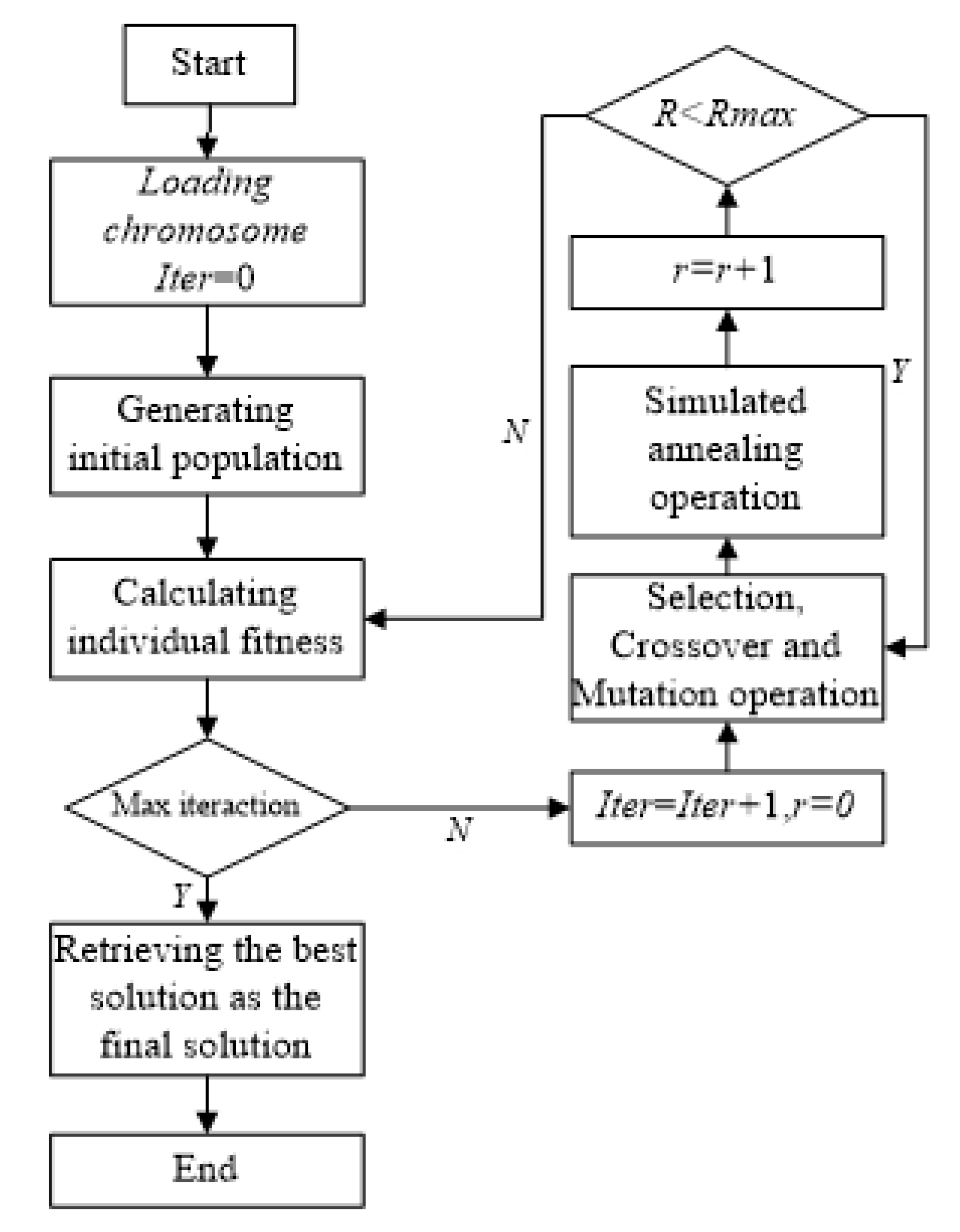
5. Solution Methodology

The above optimization model is nonlinear based on the discrete independent variables and the number of variables is big in a real case. Therefore, heuristic algorithms are needed to solve the problem. Genetic algorithm is a well-known meta-heuristic algorithm that can effectively find near-optimum solutions of scheduling problems [42,43,54,55]. It can avoid the shortcomings that exist in classical local search algorithms on difficult search spaces [56]. It has the advantage of flexibility that there is no special requirement to the form of the problem. It can also be easily combined with exact solution algorithms and local search algorithm to improve the convergence patterns [48]. Considering the characteristics of this model, a hybrid genetic algorithm based on simulated annealing (SAGA) is designed to solve the model. The idea of simulated annealing is introduced into the evolution process of genetic algorithm to alleviate the selection pressure of genetic algorithm and enhance the global search ability of genetic algorithm. The implementation procedure of adaptive genetic algorithm is shown in Figure 5, and the main steps are as follows.
Step1: Coding method and population initialization. The chromosome is composed of the starting and ending points of the truck arrival time window of vessels, and each is coded by integer numbers. A chromosome can be represented as ( p 2 S , p 2 S , , p Z S , p 1 E , p 2 E , , p Z E ) . This paper adopts the approach of initializing individuals randomly under the constraint of constraints (10)–(12), ensuring that every individual is feasible.
Step 2: Fitness evaluation and parent selection. Calculate the total carbon dioxide emissions of truck fleet and RTGCs during idling, taking the reciprocal value of total carbon dioxide emissions of truck fleet and RTGCs during idling as the fitness value. To select a parent, a roulette wheel approach is applied. The highest fitness individual of current population is retained to the next generation to ensure that the final outcome of GA is the highest fitness individual of all generations.
Step 3: Crossover. In this paper, the multi-point crossover is employed, and the specific process is shown in Figure 6.
Step 4: Mutation. In this study, the single-point mutation operator is applied. The gene values at the variation points are regenerated randomly according to the method of initial population generation.
Step 5: Offspring acceptance. After implementing the mutation operation, some offspring might don’t meet the constraints (15) and (30). These individuals are replaced by feasible ones, which are randomly generated.
Step 6: Simulated annealing operation. Simulated annealing operation is conducted after cross-mutation. Using the cooling operation T e m p = T e m p 0 d I t e r 1 , T e m p is the current temperature, T e m p 0 is the initial temperature, d is the cooling coefficient, and I t e r is the genetic algebra. Each temperature is iterated R max times. Calculating the maximal fitness in the new population m a x ( F i t n e w ) and in the original population m a x ( F i t o l d ) , respectively. If m a x ( F i t n e w ) m a x ( F i t o l d ) , the new population is taken as the initial population of the next annealing iteration. If m a x ( F i t n e w ) < m a x ( F i t o l d ) , the new population is accepted as the initial population of the next annealing iteration by probability e m a x ( F i t n e w ) m a x ( F i t o l d ) T e m p .
Step 7: Stoppage rules. An experimentally-determined maximum elapsed generation is used as the termination rule. The optimal individual of each generation is regarded as the result of genetic algorithm.

6. Numerical Experiments

In this section, the proposed optimization model is tested using the data provided by the Dalian container terminal (DCT), which has seven special container berths, 18 gate lanes, and 38 RTGCs. The DCT is a quay-type container terminal. Its layout is shown in Figure 7. This paper takes 44 vessels, calling at the port during the period 21–27 July 2014, as an example, and collects the related export containers and trucks information to conduct the research on the gate–yard queuing system by using the established queuing model in the paper. The export containers of 44 vessels were stored at 19 blocks, respectively. Since the container vessels almost provide weekly liner service, the planning horizon is set to seven days. With the travel time of trucks from the outside yard to the terminal considered, the length of appointment period is set to 0.5 h, and then the number of appointment periods is set to P = 336 . When m is set to 60, the accuracy of the model can be well ensured and is almost the same with m = 600 , but when m is smaller than 60, the accuracy falls sharply [8]. In order to guarantee the accuracy and calculation efficiency of the model, T is set to T = 5040 . The other input variables and the input values are shown in Table 2. Note that the emission factor c o comes from the Inventory of Air Emissions 2018 by POLA [57]. A RTGC consumed 5 kg/h of diesel oil while idling [58]. The emission factor c R is calculated by multiplying the diesel oil consumption, 5 kg/h, by the carbon density of diesel oil, 3.0959 kg CO2-e/kg. The estimated arrival and departure time of vessels and storage position of export containers are shown in Table 3. The maximum storage capacity of each block is shown in Table 4.

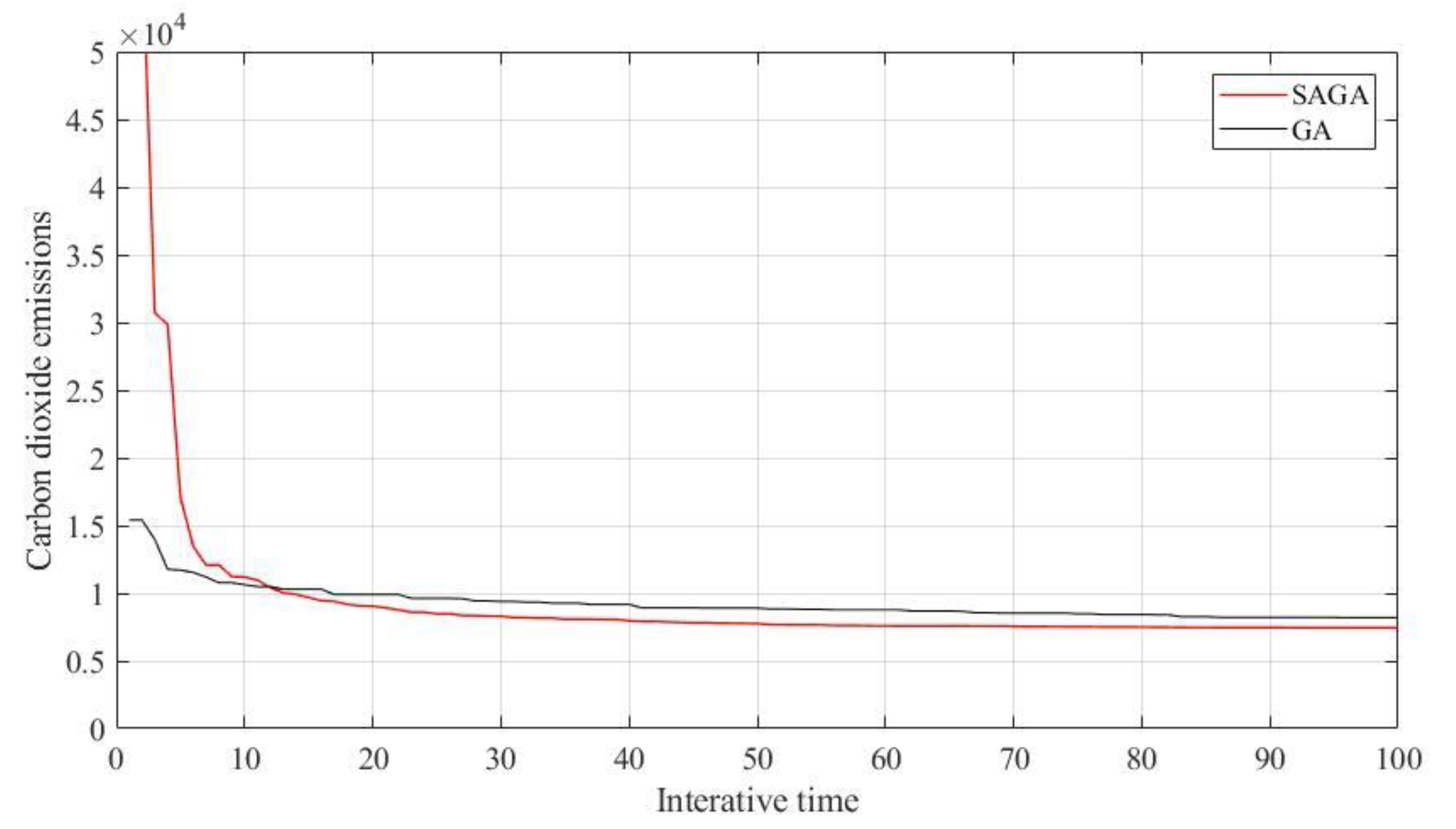
6.1. Algorithms Comparison

To test the applicability of the adopted M(t)/M/1 and M(t)/G/K truck queuing model and the proposed genetic algorithm, the simulation code is implemented in Matlab R2014a and performed based on a PC with four Intel Core i7 @ 3.2 GHz processors and 8 GB RAM. SAGA algorithm and GA algorithm use the same example and genetic parameters. The maximum length of time window for export containers of one vessel delivering T k is set to 24 h. The number of RTGCs deployed to one block is set to K = 1.
The GA parameters population size, crossover probability, mutation probability, and maximum elapsed generation are set as 160, 0.6, 0.3, and 100, respectively. The simulated annealing parameters are set to T e m p 0 = 2000 , d = 0.9 , and R max = 10 . Population size, maximum elapsed generation, and temperature iterated times are determined by trying some pilot calculations in which it is observed that these parameters are set sufficient. We carried out 12 groups of experiments to discuss the effect of parameter settings of crossover probability and mutation probability on the performance. Each setting of parameters is run for 10 times, and the average results of experiments are shown in Table 5. It is obvious that the best parameter settings of crossover probability and mutation probability for the algorithm are 0.6 and 0.3.
The convergence process of the population optimal value of SAGA and GA are shown in Figure 8. The population optimal value of SAGA reaches convergence in 92 generations where the minimum objective value 8599.843 is obtained. The population optimal value of GA reaches convergence in 96 generations where the minimum objective value 9473.68 is obtained. We can see that SAGA algorithm has faster convergence speed and can converge to a better solution. The introduction of simulated annealing makes the algorithm maintain the diversity of population in the evolution process and enhances the global convergence of genetic algorithm. Therefore, SAGA is chosen for solving the problem.

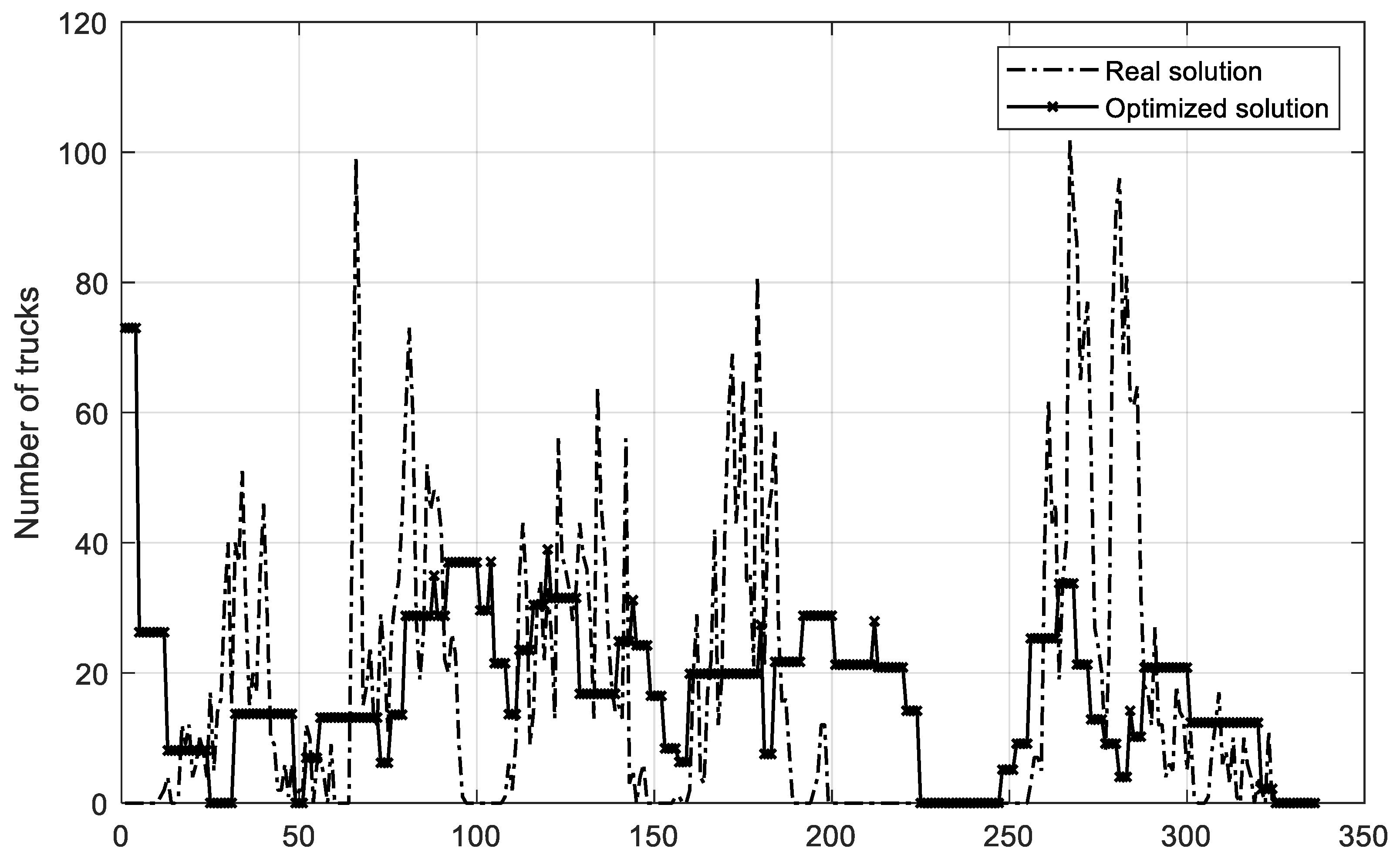
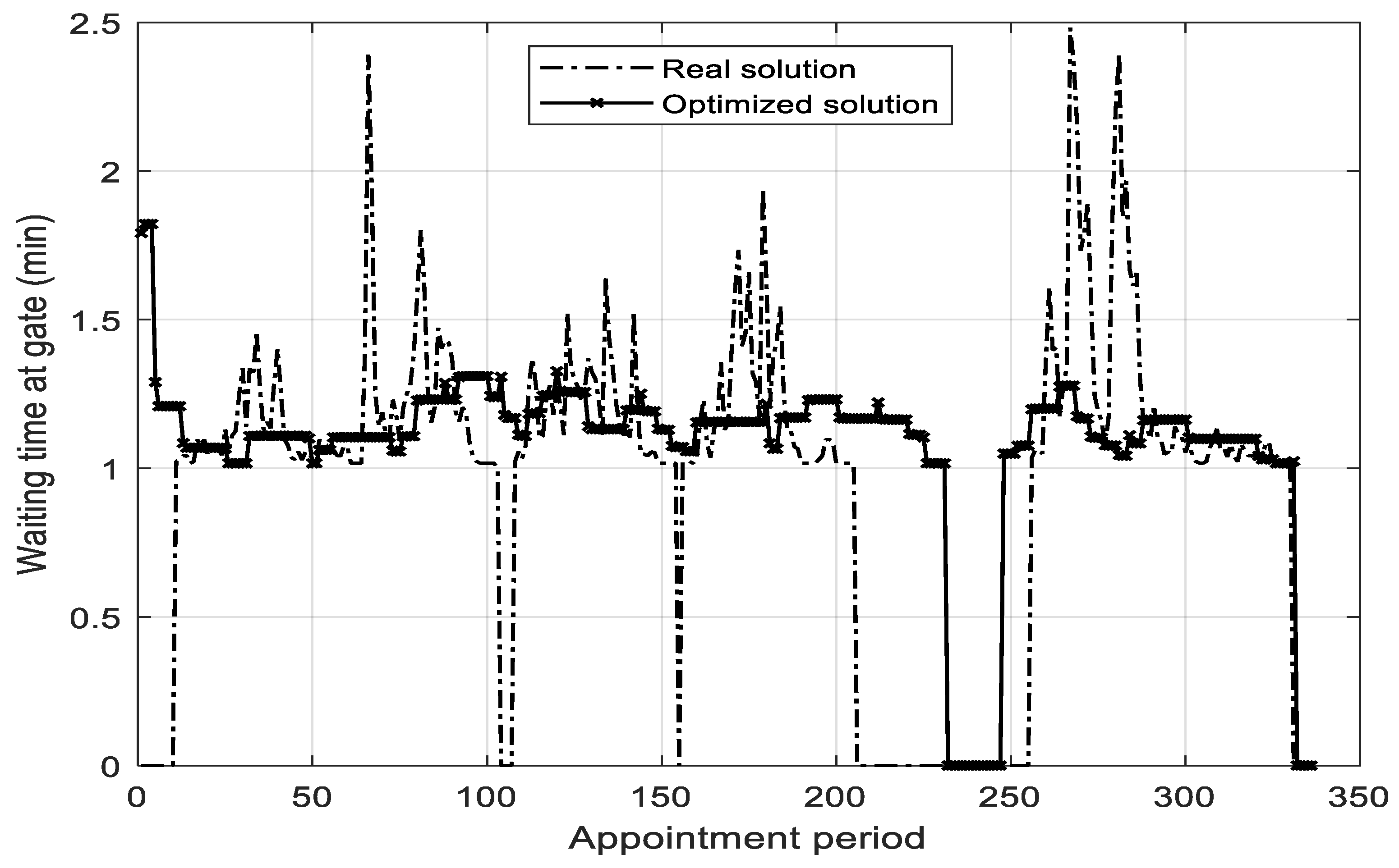
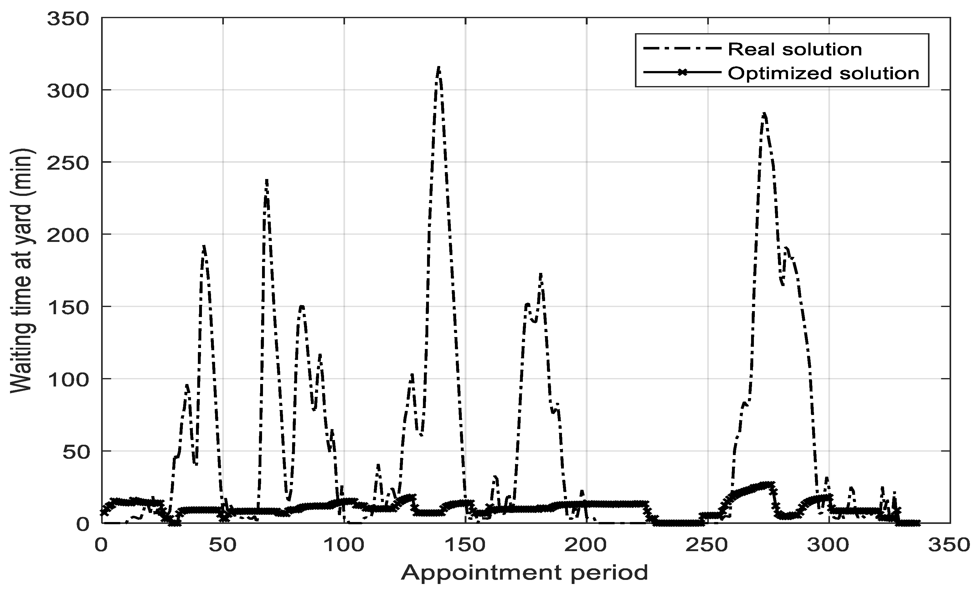
6.2. Optimization Result

Figure 9 shows the comparison between the optimized time windows and the real ones. The result indicates that the overlapping time window of vessels are greatly reduced, the total length of time windows decreases from 3410.5 h to 706 h, and the average length of time windows decreases from 77.51 h to 16.05 h. This illustrates the proposed truck arrival pattern based on the VDTWs in this paper can significantly reduce the total length of time windows and realize the concentrated arrival of vessel containers. Figure 10 compares the truck arrivals in the real and optimized solution. The result shows that the optimized truck arrival pattern based on the VDTWs can reduce the regularity of the truck arrivals and flatten the peaks of hourly truck arrivals.
Figure 11 shows the variation of average waiting time of trucks at gate. The average waiting time of trucks at gate is reduced from 1.492 min to 1.2142 min, and the longest waiting time decreases from 2.481 min to 1.8218 min, which illustrates the optimized truck arrival pattern can substantially reduce the waiting time of trucks at gate. The results show that the number of gate lanes in the DCT is sufficient to meet the needs of truck arrivals. When the terminal does not take control measures, it is not an obvious phenomenon for trucks to queue at gate. Therefore, this optimization model is not obvious to reduce the queuing length of trucks at the terminal gate. However, due to the uneven distribution of truck arrivals in the different blocks after entering the gate and the lack of RTGCs at yard, queuing at the yard is the bottleneck of affecting the truck arrivals. Figure 12 shows the variation of average waiting time of trucks at the busiest block after using the optimized truck arrival pattern. The average waiting time of trucks at yard is reduced from 54.9811 min to 9.3241 min, and the longest waiting time of the busiest block decreases from 316.2273 min to 26.7109 min, which illustrates the optimized truck arrival pattern can significantly cut down the waiting time of trucks at yard. Under the optimized truck arrival pattern, the arrival flow of trucks at the yard zone tends to be more stationary, which can effectively alleviate the yard congestion. However, due to the unbalanced distribution of truck arrivals in the different blocks, there are still some very busy blocks that trucks need to wait for a long time there.
In addition, the total carbon dioxide emissions of truck fleet and RTGCs while idling of original solution is 31493.225 kg, the total carbon dioxide emissions of truck fleet and RTGCs while idling of optimized solution is 8599.843 kg. Especially, the carbon dioxide emissions of RTGCs while idling decreases from 7804.073 kg to 3075.997 kg.

6.3. Scenario Analysis

Under the optimized truck arrival pattern, truck fleet and container terminal both benefit from the cooperative game relationship, and a container terminal gains much more profit than truck fleet. The number of RTGCs deployed to each block directly determines the model of the yard queuing system and has a great influence on the queuing time of trucks at the yard. Moreover, the appointment quota of each period depends on the length of time window. To check the influence of K and T k on the optimization result, we assume that the value of K can vary from 1 to 2 and the value of T k can vary from 8 to 48. This assumption generates 12 scenarios. The SAGA runs for all these scenarios, and the optimization results are shown in Table 6. The results indicate that increasing the length of time window for export containers delivering and the number of RTGCs can effectively cut down the waiting time of trucks at yard and reduce carbon dioxide emissions of trucks at yard significantly. However, this will lead to a reduction in the utilization rate of the RTGCs and an increase in the carbon dioxide emissions of the RTGCs. Especially, due to the uneven distribution of truck arrivals in the different blocks, an indiscriminate increase in the number of RTGCs will result in more serious idle problem of the block with very few truck arrivals. Therefore, it is necessary for the marine container terminals to control the maximum length of time window for export containers of one vessel delivering and the number of RTGCs deployed to each block.
In order to alleviate the congestion in the terminal yard effectively, we present constraints on the permissible maximum queue length γ . To check the influence of γ on the optimization result, we set different values for γ and generate 16 scenarios. The optimization results that are shown in Table 7 indicate that restraining the permissible maximum queue length can effectively control the congestion in the terminal yard. Furthermore, decreasing the value of γ can cut down the waiting time of trucks at yard and reduce carbon dioxide emissions of trucks at yard. In order to reduce the waiting time of trucks at each block, a longer time window should be set up for vessels with a large number of truck arrivals. Therefore, this will lead to a reduction in the utilization rate of the RTGCs and an increase in the carbon dioxide emissions of the RTGCs.

7. Conclusions

The irregular arrival of trucks is a key factor that leads to the congestion at gate and yard and affects the efficiency of receiving and delivery operations at the marine container terminal. Considering that container arrivals are triggered by vessel arrival process, this paper proposes a new terminal appointment system with VDTWs. On the basis of existing studies about TAS, this paper establishes an optimization model for container delivery to determine the truck arrival time window for each vessel and the appointment quota of each period for each vessel to minimize the total carbon dioxide emissions of truck fleet and RTGCs. The storage space constraints of each block and the constraint of maximum queue length are taken into account according to reality. A hybrid genetic algorithm based on simulated annealing is developed to solve this model. In the genetic algorithm, the application of the simulated annealing operation can accelerate the search process and ensure that the algorithm eventually converges to the global optimal solution. Taking Dalian container terminal as an example, a numerical experiment is conducted. The result indicates that without terminal expansion and purchase of additional machinery, implementing the optimized truck arrival pattern can significantly alleviate congestion at gate and yard and reduce carbon dioxide emissions trucks at yard significantly. Increasing the number of RTGCs and the length of the time window for export containers delivering can effectively reduce the waiting time of trucks at yard and reduce carbon dioxide emissions of trucks. However, this will reduce the utilization rate of the RTGCs and increase the carbon dioxide emissions of the RTGCs. Therefore, it is necessary for marine container terminal operators to control the maximum length of the time window for export containers delivering by one vessel and the number of RTGCs deployed to each block. The outcomes can provide decision-making basis for TAS development in marine container terminals.
In the model built in this paper, the number of RTGCs deployed to each block is fixed. However, the distribution of truck arrivals between different blocks is uneven. If we blindly adopt the method of purchasing RTGCs and increase the number of RTGCs deployed to each block to reduce the waiting time of delivery trucks, it does not only need a lot of money to be invested in, but also causes waste of crane capacity. In future research, we can utilize the advantage of the RTGC that it can be moved from one block to another flexibly. We can determine the number of RTGCs to be deployed in each block and a scheduling plan of RTGCs according to the workload of each block under the optimized truck arrival pattern. It can both reduce the queuing and improve the utilization rate of the RTGCs. Therefore, further research needs to consider the scheduling problem of RTGCs and determine the appropriate number of RTGCs deployed to the yard.

Author Contributions

Data curation, Z.G.; investigation, X.J.; formal analysis, X.J. and Z.G.; methodology, M.M.; validation, M.M. and H.F.; supervision, H.F.; writing—original draft, M.M.; writing—review & editing, H.F. and X.J.

Funding

National Natural Science Foundation of China: 61473053, 71971035. Liaoning Social Science Planning Fund: L19BGL006.

Acknowledgments

The authors gratefully acknowledge the financial support received from the National Natural Science Foundation of China grant coded: 61473053. In addition, the authors would like to thank the Dalian container terminal for providing data for this research. The authors also would like to thank the strong administration support rendered by the MDPI editorial team.

Conflicts of Interest

The authors declare no conflicts of interest.

References

  1. Wan, C.; Yan, X.; Zhang, D.; Qu, Z.; Yang, Z. An advanced fuzzy Bayesian-based FMEA approach for assessing maritime supply chain risks. Transp. Res. E-Logist. 2019, 125, 222–240. [Google Scholar] [CrossRef]
  2. UNCTAD. Review of Maritime Transport; United Nations Conference on Trade and Development: New York, NY, USA; Geneva, Switzerland, 2019. [Google Scholar]
  3. Xiang, X.; Liu, C.; Miao, L. Reactive strategy for discrete berth allocation and quay crane assignment problems under uncertainty. Comput. Ind. Eng. 2018, 126, 196–216. [Google Scholar] [CrossRef]
  4. Munim, Z.H.; Schramm, H.J. The impacts of port infrastructure and logistics performance on economic growth: The mediating role of seaborne trade. J. Ship. Trade 2018, 3, 1–19. [Google Scholar] [CrossRef]
  5. IMO. Third IMO GHG Study 2014. Available online: http://www.imo.org/en/OurWork/Environment/PollutionPrevention/AirPollution/Pages/Greenhouse-Gas-Studies-2014.aspx (accessed on 2 November 2018).
  6. Dulebenets, M.A. Green vessel scheduling in liner shipping: Modeling carbon dioxide emission costs in sea and at ports of call. Int. J. Transp. Sci. Technol. 2018, 7, 26–44. [Google Scholar] [CrossRef]
  7. Peng, Y.; Wang, W.; Song, X.; Zhang, Q. Optimal allocation of resources for yard crane network management to minimize carbon dioxide emissions. J. Clean. Prod. 2016, 131, 649–658. [Google Scholar] [CrossRef]
  8. Chen, X.; Zhou, X.; List, G.F. Using time-varying tolls to optimize truck arrivals at ports. Transp. Res. E-Logist. 2011, 47, 965–982. [Google Scholar] [CrossRef]
  9. Wagner, I. Container Shipping—Statistics & Facts. Available online: https://www.statista.com/topics/1367/container-shipping/ (accessed on 2 November 2018).
  10. Lalla-Ruiz, E.; Expósito-Izquierdo, C.; Melián-Batista, B.; Moreno-Vega, J.M. A set-partitioning-based model for the berth allocation problem under time-dependent limitations. Eur. J. Oper. Res. 2016, 250, 1001–1012. [Google Scholar] [CrossRef]
  11. Ursavas, E.; Zhu, S.X. Optimal policies for the berth allocation problem under stochastic nature. Eur. J. Oper. Res. 2016, 255, 380–387. [Google Scholar] [CrossRef]
  12. Zhen, L.; Liang, Z.; Zhuge, D.; Lee, L.H.; Chew, E.P. Daily berth planning in a tidal port with channel flow control. Transp. Res. B-Methodol. 2017, 106, 193–217. [Google Scholar] [CrossRef]
  13. Fonseca, G.B.; Nogueira, T.H.; Ravetti, M.G. A hybrid Lagrangian metaheuristic for the cross-docking flow shop scheduling problem. Eur. J. Oper. Res. 2019, 275, 139–154. [Google Scholar] [CrossRef]
  14. Lee, B.K.; Kim, K.H. Comparison and evaluation of various cycle-time models for yard cranes in container terminals. Int. J. Prod. Econ. 2010, 126, 350–360. [Google Scholar] [CrossRef]
  15. Dulebenets, M.A. The vessel scheduling problem in a liner shipping route with heterogeneous fleet. Int. J. Civ. Eng. 2018, 16, 19–32. [Google Scholar] [CrossRef]
  16. Motono, I.; Furuichi, M.; Ninomiya, T.; Suzuki, S.; Fuse, M. Insightful observations on trailer queues at landside container terminal gates: What generates congestion at the gates? Res. Transp. Bus. Manag. 2016, 19, 118–131. [Google Scholar] [CrossRef]
  17. Giuliano, G.; O’Brien, T. Reducing port-related truck emissions: The terminal gate appointment system at the Ports of Los Angeles and Long Beach. Transp. Res. D-TR. E 2007, 12, 460–473. [Google Scholar] [CrossRef]
  18. Mani, A.; Fischer, M.J. FHWA Operations Support-Port Peak Pricing Program Evaluation; Federal Highway Administration: Washington, DC, USA, 2009.
  19. Zeng, Q.; Chen, W.; Huang, L. A model and its algorithms for truck congestion toll at container terminals. J. Dalian Univ. Technol. 2015, 55, 73–80. [Google Scholar]
  20. Sharif, O.; Huynh, N.; Vidal, J.M. Application of El Farol model for managing marine terminal gate congestion. Res. Transp. Econ. 2011, 32, 81–89. [Google Scholar] [CrossRef]
  21. Chen, G.; Govindan, K.; Yang, Z. Managing truck arrivals with time windows to alleviate gate congestion at container terminals. Int. J. Prod. Econ. 2013, 141, 179–188. [Google Scholar] [CrossRef]
  22. Wei, H. Optimal pickup time windows allocation at container terminal. J. Manag. Sci. China 2011, 14, 21–36. [Google Scholar]
  23. Chen, G.; Jiang, L. Managing customer arrivals with time windows: A case of truck arrivals at a congested container terminal. Ann. Oper. Res. 2016, 244, 349–365. [Google Scholar] [CrossRef]
  24. Guo, Z.; Fan, H.; Ma, M.; Li, Y. Optimization model for appointment of delivery trucks based on vessel dependent time windows. Ind. Eng. Manag. 2017, 22, 24–30. [Google Scholar]
  25. Morais, P.; Lord, E. Terminal Appointment System Study; Canada Csa Final Report Copy: Montreal, QC, Canada, 2006.
  26. Huynh, N.; Walton, C.M. Robust scheduling of truck arrivals at marine container terminals. J. Transp. Eng. 2008, 134, 347–353. [Google Scholar] [CrossRef]
  27. Namboothiri, R.; Erera, A.L. Planning local container drayage operations given a port access appointment system. Transp. Res. E-Logist. 2008, 44, 185–202. [Google Scholar] [CrossRef]
  28. Kim, K.H.; Kim, H.B. The optimal sizing of the storage space and handling facilities for import containers. Transp. Res. B-Methodol. 2002, 36, 821–835. [Google Scholar] [CrossRef]
  29. Guan, C.; Liu, R.R. Container terminal gate appointment system optimization. Marit. Econ. Logist. 2009, 11, 378–398. [Google Scholar] [CrossRef]
  30. Zeng, Q.C.; Zhang, X.J.; Chen, W.H.; Zhu, X.C. Optimization model for truck appointment based on BCMP queuing network. J. Syst. Eng. 2013, 28, 592–599. [Google Scholar]
  31. Zhang, X.; Zeng, Q.; Chen, W. Optimization Model for Truck Appointment in Container Terminals. Proc.-Soc. Behav. Sci. 2013, 96, 1938–1947. [Google Scholar] [CrossRef]
  32. Xu, Q.L.; Sun, L.J.; Hu, X.P.; Wu, R.L. Optimization model for appointment of container trucks with non-stationary arrivals. J. Dalian Univ. Technol. 2014, 54, 589–596. [Google Scholar]
  33. Zhang, X.; Zeng, Q.; Chen, W. Optimization model of terminal container truck appointment based on coordinated service of inner and outer container trucks. J. Traffic Transp. Eng. 2016, 16, 115–122. [Google Scholar]
  34. Jiang, M.; Zhang, X.; Feng, D.; Cai, Q.; Wang, Z. Study on appointment scheduling model of container port truck based on poisson process. J. Zhejiang Univ. Technol. 2016, 44, 292–298. [Google Scholar]
  35. Yang, H.; Shao, Q.; Geng, F.; Jin, Z. Collaborative optimization of yard crane deployment and truck appointment based on two-way transmission of information. J. Dalian Maritime Univ. 2017, 43, 29–38. [Google Scholar]
  36. Ma, M.; Fan, H.; Ji, M.; Guo, Z. Integrated Optimization of Truck Appointment for Export Containers and Crane Deployment in a Container Terminal. J. Transp. Syst. Eng. Inf. Technol. 2018, 18, 202–209. [Google Scholar]
  37. Goldsworthy, L.; Goldsworthy, B. Modelling of ship engine exhaust emissions in ports and extensive coastal waters based on terrestrial AIS data—An Australian case study. Environ. Model. Softw. 2015, 63, 45–60. [Google Scholar] [CrossRef]
  38. López-Aparicio, S.; Tønnesen, D.; Thanh, T.N.; Neilson, H. Shipping emissions in a Nordic port: Assessment of mitigation strategies. Transport. Res. D-TR. E 2017, 53, 205–216. [Google Scholar] [CrossRef]
  39. Nunes, R.A.O.; Alvim-Ferraz, M.C.M.; Martins, F.G.; Sousa, S.I.V. Assessment of shipping emissions on four ports of Portugal. Environ. Pollut. 2017, 231, 1370–1379. [Google Scholar] [CrossRef] [PubMed]
  40. Yu, H.; Ge, Y.E.; Chen, J.; Luo, L.; Tan, C.; Liu, D. CO2 emission evaluation of yard tractors during loading at container terminals. Transp. Res. D-TR. E 2017, 53, 17–36. [Google Scholar] [CrossRef]
  41. Liu, D.; Ge, Y.E. Modeling assignment of quay cranes using queueing theory for minimizing CO2 emission at a container terminal. Transp. Res. D-TR. E 2018, 61, 140–151. [Google Scholar] [CrossRef]
  42. Hu, X.; Guo, J.; Zhang, Y. Optimal strategies for the yard truck scheduling in container terminal with the consideration of container clusters. Comput. Ind. Eng. 2019, 137, 106083. [Google Scholar] [CrossRef]
  43. Han, X.L.; Wang, Q.; Huang, J.W. Scheduling cooperative twin automated stacking cranes in automated container terminals. Comput. Ind. Eng. 2019, 128, 553–558. [Google Scholar] [CrossRef]
  44. Yang, Y.C.; Chang, W.M. Impacts of electric rubber-tired gantries on green port performance. Res. Transp. Bus. Manag. 2013, 8, 67–76. [Google Scholar]
  45. Berechman, J.; Tseng, P.H. Estimating the environmental costs of port related emissions: The case of Kaohsiung. Transp. Res. D-TR. E 2012, 17, 35–38. [Google Scholar] [CrossRef]
  46. Gibbs, D.; Rigot-Muller, P.; Mangan, J.; Lalwani, C. The role of sea ports in end-to-end maritime transport chain emissions. Energy Policy 2014, 64, 337–348. [Google Scholar] [CrossRef] [Green Version]
  47. Sim, J. A carbon emission evaluation model for a container terminal. J. Clean. Prod. 2018, 186, 526–533. [Google Scholar] [CrossRef]
  48. Chen, G.; Govindan, K.; Golias, M.M. Reducing truck emissions at container terminals in a low carbon economy: Proposal of a queueing-based bi-objective model for optimizing truck arrival pattern. Transp. Res. E-Logist. 2013, 55, 3–22. [Google Scholar] [CrossRef]
  49. Brown, L.; Gans, N.; Mandelbaum, A.; Sakov, A.; Shen, H.; Zeltyn, S.; Zhao, L. Statistical analysis of a telephone call center: A queueing-science perspective. J. Am. Stat. Assoc. 2005, 100, 36–50. [Google Scholar] [CrossRef] [Green Version]
  50. Kim, S.H.; Whitt, W. Choosing arrival process models for service systems: Tests of a nonhomogeneous Poisson process. Nav. Res. Log. 2014, 61, 66–90. [Google Scholar] [CrossRef]
  51. Stewart, W.J. Probability, Markov Chains, Queues, and Simulation: The Mathematical Basis of Performance Modeling; Princeton University Press: Princeton, NJ, USA, 2009; pp. 560–562. [Google Scholar]
  52. Ji, X.; Zhang, J.; Ran, B.; Ban, X.G. Fluid Approximation of Point-queue Model. Proc.-Soc. Behav. Sci. 2014, 38, 470–481. [Google Scholar] [CrossRef] [Green Version]
  53. Wang, W.P.; Tipper, D.; Banerjee, S. A simple approximation for modeling nonstationary queues. In Proceedings of the Fifteenth Annual Joint Conference of the IEEE Computer Societies, San Francisco, CA, USA, 24–28 March 1996. [Google Scholar]
  54. Homayouni, S.M.; Tang, S.H.; Motlagh, O. A genetic algorithm for optimization of integrated scheduling of cranes, vehicles, and storage platforms at automated container terminals. J. Comput. Appl. Math. 2014, 270, 545–556. [Google Scholar] [CrossRef]
  55. Yang, Y.; Zhong, M.; Dessouky, Y.; Postolache, O. An integrated scheduling method for AGV routing in automated container terminals. Comput. Ind. Eng. 2018, 126, 482–493. [Google Scholar] [CrossRef]
  56. Skinner, B.; Yuan, S.; Huang, S.; Liu, D.; Cai, B.; Dissanayake, G.; Lau, H.; Bott, A.; Pagac, D. Optimisation for job scheduling at automated container terminals using genetic algorithm. Comput. Ind. Eng. 2013, 64, 511–523. [Google Scholar] [CrossRef]
  57. Starcrest Consulting Group, LLC. Inventory of Air Emissions for CY 2018; Starcrest Consulting Group, LLC: Port of Los Angeles, CA, USA, 2019. [Google Scholar]
  58. Li, T. A research of the power-saving unit for the engine with double speed on the shore based container. Port Sci. Technol. 2008, 8, 40–41. [Google Scholar]
Figure 1. A two-phase queuing system in a marine container terminal.
Sustainability 11 06410 g001
Figure 2. The number of hourly truck arrivals.
Sustainability 11 06410 g002
Figure 3. The histogram of frequency distribution of gate service time.
Sustainability 11 06410 g003
Figure 4. The histogram of frequency distribution of rubber-tired gantry cranes (RTGCs) service time.
Sustainability 11 06410 g004
Figure 5. Implementation procedure of simulated annealing (SAGA).
Sustainability 11 06410 g005
Figure 6. Representation of crossover.
Sustainability 11 06410 g006
Figure 7. The layout of the Dalian container terminal (DCT).
Sustainability 11 06410 g007
Figure 8. Convergence process of SAGA and genetic algorithm (GA).
Sustainability 11 06410 g008
Figure 9. The time window assignment in the real and optimized cases.
Sustainability 11 06410 g009
Figure 10. The truck arrivals in the real and optimized cases.
Sustainability 11 06410 g010
Figure 11. The truck waiting time at gate in the real and optimized cases.
Sustainability 11 06410 g011
Figure 12. The truck waiting time at the busiest block in the real and optimized cases.
Sustainability 11 06410 g012
Table 1. The p-values of the CU KS test and Log KS test of a non-homogeneous Poisson process (NHPP).
Time n b CU KS TestLog KS Test
L = 0.5 h L = 1 h L = 0.5 h L = 1 h
14 July 00:00–14 July 18:002560.1313 0.1477 0.5864 0.0013
14 July 18:00–15 July 10:002790.0893 0.0338 0.1224 0.3453
15 July 10:00–15 July 14:002600.6514 0.2116 0.0393 0.0414
15 July 14:00–15 July 18:002390.1959 0.0882 0.1418 0.0499
15 July 18:00–16 July 8:002420.2667 0.0000 0.0235 0.0069
16 July 8:00–16 July 12:002400.1226 0.0104 0.1052 0.0034
16 July 12:00–16 July 18:002590.1545 0.7477 0.4571 0.7642
16 July 18:00–16 July 24:002010.3556 0.1693 0.0371 0.0003
16 July 24:00–17 July 12:002750.3341 0.6114 0.0000 0.0533
17 July 12:00–17 July 16:002570.2871 0.6779 0.5132 0.2111
17 July 16:00–17 July 24:002910.4680 0.0142 0.0831 0.0005
17 July 24:00–18 July 12:001890.1157 0.1052 0.2708 0.1346
18 July 12:00–18 July 16:004090.0015 0.0589 0.0871 0.0864
18 July 16:00–18 July 18:002960.6989 0.9450 0.0003 0.0001
18 July 18:00–18 July 20:002800.6393 0.8370 0.0073 0.0027
18 July 20:00–19 July 8:001960.6027 0.0004 0.6730 0.2958
19 July 8:00–19 July 10:003340.6304 0.4638 0.0101 0.0011
19 July 10:00–19 July 12:003200.1582 0.0196 0.0454 0.0576
19 July 12:00–19 July 14:002700.8721 0.7229 0.1451 0.0711
19 July 14:00–19 July 24:002490.1398 0.0347 0.2931 0.1547
19 July 24:00–20 July 12:003590.1922 0.0107 0.1247 0.0481
20 July 12:00–20 July 16:003050.5903 0.0871 0.2279 0.5239
20 July 16:00–21 July 12:002170.4831 0.0394 0.1008 0.0043
21 July 12:00–21 July 18:002480.3520 0.4404 0.6264 0.6919
21 July 18:00–22 July 8:002090.1533 0.2846 0.4561 0.0497
22 July 8:00–22 July 14:003870.0024 0.0058 0.5323 0.1792
22 July 14:00–22 July 18:003320.1614 0.0382 0.0904 0.0764
22 July 18:00–22 July 24:002740.0027 0.0007 0.0679 0.4879
22 July 24:00–23 July 12:002360.8998 0.3438 0.2641 0.0173
23 July 12:00–23 July 16:002200.8784 0.8289 0.1710 0.2525
23 July 16:00–23 July 20:002710.1168 0.0209 0.0891 0.0663
23 July 20:00–24 July 10:002470.0931 0.0042 0.2227 0.2424
24 July 10:00–24 July 14:002320.3408 0.0660 0.0036 0.0074
24 July 14:00–24 July 18:003680.9951 0.0867 0.5613 0.1891
24 July 18:00–25 July 2:001920.1361 0.1686 0.0923 0.3122
25 July 2:00–26 July 13:002810.00000.0024 0.0778 0.8467
26 July 13:00–26 July 15:003160.9903 0.3096 0.0190 0.0134
26 July 15:00–26 July 18:002650.4963 0.4893 0.4485 0.3692
26 July 18:00–26 July 21:004790.0669 0.1102 0.0000 0.0000
26 July 21:00–26 July 23:002770.2232 0.0386 0.2257 0.2848
26 July 23:00–27 July 8:003010.8806 0.1596 0.0013 0.0048
27 July 8:00–27 July 10:003430.5620 0.5131 0.0021 0.0029
27 July 10:00–27 July 12:002450.2238 0.2189 0.1113 0.1704
27 July 12:00–27 July 24:002690.2197 0.0403 0.2381 0.0446
Table 2. Values of the input variables in the optimization model.
Input Variable c o
(kg/h)
c R
(kg/h)
u i t g
(truck/h)
u j k t y
(container/h)
C s T l
(h)
α I
Value5.72815.4859190.4268761.44
Table 3. The estimated arrival and departure time of vessels and storage position of export containers.
Vessel No. T z A T z D Block No.Number of Containers Stacked (Natural Container)
121 July 2014 5:0021 July 2014 15:309100
221 July 2014 1:0021 July 2014 10:301111
321 July 2014 10:0021 July 2014 22:301234
421 July 2014 14:3022 July 2014 1:009159
521 July 2014 19:3022 July 2014 9:3014239
621 July 2014 21:3022 July 2014 8:3012224
721 July 2014 23:3022 July 2014 8:001186
822 July 2014 8:3022 July 2014 23:307273
922 July 2014 9:0023 July 2014 2:0016247
1022 July 2014 16:0023 July 2014 7:0015135
1694
1122 July 2014 17:0023 July 2014 13:00286
1222 July 2014 23:0023 July 2014 13:004204
1323 July 2014 5:3023 July 2014 15:004107
1423 July 2014 15:0024 July 2014 7:0012123
17110
1523 July 2014 17:0024 July 2014 7:30385
565
1623 July 2014 17:0024 July 2014 1:001977
1723 July 2014 19:3024 July 2014 7:0010155
1823 July 2014 22:0024 July 2014 8:0017146
1924 July 2014 1:0024 July 2014 13:00592
2024 July 2014 5:0024 July 2014 17:0011227
2124 July 2014 13:0025 July 2014 0:008253
2224 July 2014 16:3025 July 2014 5:30194
2324 July 2014 17:3025 July 2014 5:0018214
2426 July 2014 19:0027 July 2014 11:008109
2527 July 2014 10:3028 July 2014 0:0011157
16253
2626 July 2014 20:0027 July 2014 6:006158
2726 July 2014 21:3027 July 2014 14:0013202
2826 July 2014 20:3027 July 2014 9:3011171
2926 July 2014 21:0027 July 2014 9:3017233
3026 July 2014 22:3027 July 2014 12:3010149
3126 July 2014 22:3027 July 2014 12:301460
3227 July 2014 8:3028 July 2014 0:00344
9157
3327 July 2014 6:0028 July 2014 0:004169
3427 July 2014 10:0028 July 2014 0:007127
3527 July 2014 12:3027 July 2014 22:0014105
3627 July 2014 13:0028 July 2014 3:0010155
13130
3727 July 2014 18:3028 July 2014 8:001576
3827 July 2014 19:0028 July 2014 6:002132
3927 July 2014 20:0028 July 2014 10:001160
3127
4027 July 2014 21:3028 July 2014 6:00478
4127 July 2014 22:0028 July 2014 12:3016180
18197
4227 July 2014 22:3028 July 2014 13:301680
4327 July 2014 23:3028 July 2014 14:30253
4427 July 2014 23:3028 July 2014 10:009110
Table 4. The maximum storage capacity of each block.
Block No.12345678910
Maximum storage capacity500500500500500500500500500550
Block No.111213141516171819
Maximum storage capacity550550550550520520520520300
Table 5. The performance comparison of different parameters setting.
No.Crossover ProbabilityMutation ProbabilityAverage Results
10.60.17887.253
20.60.27858.244
30.60.37791.335
40.70.17843.657
50.70.27845.88
60.70.37791.428
70.80.17822.194
80.80.27807.571
90.80.37802.982
100.90.17852.937
110.90.27817.444
120.90.37837.182
Table 6. The effect of K and T k on the queuing system.
Scenario No.Number of RTGCs Deployed to Each Block
K
The Maximum Length of Time Window
T k
The Total Carbon Dioxide Emissions
(kg)
The Carbon Dioxide Emissions of Trucks at Gate
(kg)
The Carbon Dioxide Emissions of Trucks at Yard
(kg)
The Carbon Dioxide Emissions of RTGCs
(kg)
11855,361.431926.0751,819.581615.78
211218,913.05576.5716,224.772111.71
31188751.04488.795646.062616.19
41248599.837470.175053.673075.9974
51368593.95461.384494.953637.62
61488333.68457.514059.663816.51
72876,642.46622.474,139.151880.91
821245,763.35613.3742,331.92818.08
921824,638.44606.8819,184.194847.37
1022421,694.44610.514,458.026625.92
1123623,846.06606.4213,031.5910,208.05
1224823,802.27604.6812,930.6410,266.95
Table 7. The effect of γ on the queuing system.
Scenario No.Number of RTGCs Deployed to Each Block
K
The Maximum Length of Time Window
T k
The Maximum of Containers Waiting in the Queue at Each Block
γ
The Total CO2 Emissions
(kg)
The CO2 Emissions of Trucks at Gate
(kg)
The CO2 Emissions of Trucks at Yard
(kg)
The CO2 Emissions of RTGCs
(kg)
111879008.47491.445778.032739
211889093.25500.485836.822755.95
311899174.19496.626049.632627.94
4118109435.02505.436324.612604.98
5124310264.66530.824659.65074.24
612448561.13472.075202.562886.5
712459038.74483.445747.722807.58
812469100.43478.146019.022603.27
913628433.52470.534258.93704.09
1013638593.95461.384494.953637.62
1113648710.17461.484997.843250.85
1213658411.766464.0565049.132898.58
1314828333.68457.514059.663816.51
1414838920.38455.395280.413184.58
1514848826.11459.65400.462966.05
1614858848.025465.875524.0352858.12

