An Extensive Investigation of an Eco-Approach Controller under a Partially Connected and Automated Vehicle Environment

Abstract

This study evaluated the performance of an eco-approach control system at signalized intersections under a partially connected and automated vehicle (CAV) environment. This system has the first eco-approach controller able to function with the existence of surrounding human-driven traffic. A previous evaluation only confirmed its benefits. The purpose of this study was to conduct a further extensive test on the controller to identify room for improvement. Two different networks were tested, including an isolated signalized intersection and a corridor with two signalized intersections. The measures of effectiveness (MOEs) adopted were throughput and fuel consumption. All the before-and-after MOEs were compared using t-tests. The results indicate that the controller generally improved the fuel efficiency without harm to the mobility, and its environmental performance was affected by the minimum CAV speed, green ratio, congestion level, and marker penetration rate of CAVs. A detailed investigation revealed that no significant environmental benefit was generated under high congestion levels when the minimum speed of CAVs was more than 20 mph, and the shockwaves caused by the eco-approach control may result in a gating effect that reduces the throughput at the upstream intersection of the corridor under high congestion levels.

1. Introduction

As the transportation sector is a main source of greenhouse gas (GHG) emissions [1], many governments and researchers around the world have focused on fuel efficiency improvement and emission reduction [2]. A variety of approaches, including the development of clean energy and power technology [3], the improvement of traffic management and control [4], and the enhancement of vehicle operation [5], have been proposed, with some achievements made. With emerging connected and automated vehicle (CAV) technology, a brand new fuel efficiency improvement technology known as “eco-driving” has become an emerging research focus [6]. Most existing eco-driving research can be categorized into eco-driving on the freeway [7,8,9,10,11] and eco-driving on signalized arterials [12,13,14,15,16,17,18,19]. Eco-driving on the freeway mainly focuses on smoothing the vehicles’ speed profile to reduce traffic oscillations which can cause extra energy consumption and emissions. Eco-driving on signalized arterials optimizes the vehicle speed profile to avoid idling at traffic signals and reduces acceleration and deceleration maneuvers while approaching or departing intersections. The present research relates to the category of eco-driving on signalized arterials.

Most previous eco-driving strategies on signalized arterials were developed for a completely connected and automated vehicle environment, which means that these eco-driving controllers could obtain the kinematics information of all vehicles in real time and accurately control their motions [12,13,14,15]. These strategies are not feasible for real-world implementation in the near future due to their poor robustness against the impedance from conventional vehicles and the randomness of traffic [16]. To overcome this drawback, queue theory and car following theory were introduced into some eco-driving studies on signalized arterials to predict the location and motion of conventional vehicles [16,17,18,19,20,21]. It is expected that these eco-driving controllers will be functional in a partially connected and automated vehicle environment and can be implemented as long as CAV technology is introduced in the near future [17]. However, it is still difficult to affirm the limitations, risks, or benefits of these eco-driving controllers in mixed traffic flow [22]. The influences of factors on the performance of eco-driving controllers implemented on signalized arterials under a partially connected and automated vehicle environment is one of the most meaningful topics to explore [23].

Some eco-driving controllers on signalized arterials under a partially connected and automated vehicle environment have been developed for individual vehicles, and the optimization of speed profiles aims to maximize the fuel efficiency of a single CAV [12,13,14,15]. The evaluation results indicated that these controllers could generate considerable fuel consumption benefits under low saturation conditions but cause significant harm to mobility and even have some negative effects on the vehicle fuel efficiency under high saturation conditions [16]. To eliminate this limitation, some pure “win” eco-driving controllers were developed to reduce the total fuel consumption of traffic systems while doing no harm to the throughput of intersections, if not benefitting them, which could indirectly control conventional vehicles by utilizing car-following models [16,17]. The existing brief evaluations on these controllers only confirm the benefits, few limitations, and feasible conditions that they may provide for further improvement and implementation [23].

To bridge this gap, this study conducted an extensive investigation on an eco-approach controller under a partially connected and automated vehicle environment. It is the first representative controller designed for isolated signalized intersection in mixed traffic conditions which consist of CAVs and conventional human-driven vehicles [16]. The “eco-approach” refers to one of the eco-driving applications on signalized arterials, which optimizes the speed trajectories of CAVs with real-time Signal Phase and Timing (SPaT) information [12].

The objective of this research is to further investigate the impacts of various factors on the mobility and environmental performance of the eco-approach controller in multiple simulation networks to identify the feasible implementation conditions of the controller at an isolated signalized intersection, analyze the adaptation of the controller to a signalized corridor with multiple intersections, discuss the limitations and shortcomings of the controller, and provide useful information for further improvement. This research established a general investigation framework of eco-driving on signalized arterials, which could help the researchers find a further development direction for eco-driving on signalized arterials under a partially connected and automated vehicles environment.

The reminder of the paper is organized as follows: Section 2 “Literature Review” summarizes the related studies of eco-driving investigation; Section 3 “Eco-Approach Control System” briefly introduces the principles of this eco-approach controller; Section 4 “Experiment Design and Setup” describes the simulation setup and experiment design in detail; Section 5 “Results” and Section 6 “Discussion” present the simulation results and analysis process; and Section 7 “Conclusions and Future Research” entails the conclusions and guidance for future work.

2. Literature Review

To evaluate the benefits of implementing eco-driving approaches on signalized arterials, many past studies adopted simulation or field tests [2,3,13,14]. Almost every study confirmed the environmental benefits (improvements in fuel efficiency and emission reduction) of implementing eco-driving approaches on signalized arterials. In order to guide the implementation or test the robustness of these eco-driving approaches in complex traffic conditions, some studies attempted to establish a relationship between their environmental benefits and traffic-related factors [16]. Typical traffic-related factors include the congestion level (CL) and market penetration rate (MPR) of vehicles controlled by eco-driving controllers [18,20].

The results indicate that most eco-driving approaches that have attempted to minimize the fuel consumption and emissions of individual vehicles have shown decreasing trends in environmental benefits with an increase in the congestion level, and eco-driving approaches focused on improving global fuel efficiency and emission reduction could generate larger environmental benefits with an increase in the congestion level [16,17]. Under a partially connected and automated vehicles environment, the impact of the MPR of CAVs on the environmental benefits of eco-driving is relatively straightforward. Most approaches show a better performance under a higher MPR level for controlled vehicles [14,15,16,17,18,19]. Some advanced eco-driving approaches can even generate significant benefits as long as there are CAVs [16,17], which indicates that these approaches can be implemented with a low CAV MPR and could be implemented in the near future. The interactions between human-driven vehicles and CAVs show that CAVs have a positive effect on following conventional vehicles [24,25]. That is to say, the conventional vehicles could obtain approximately optimal speed profiles by following their preceding CAVs to reduce fuel consumption and emissions [16,17]. This further confirms that it is feasible to predict the motions of conventional vehicles by using car following models [16,17,18,20].

However, few studies have focused on the impacts of infrastructure-related factors on the benefits of eco-driving approaches on signalized arterials. The signal timing plan, speed limit, and link length between adjacent intersections are the most important infrastructure-related factors in the evaluations [4,5]. Most existing studies adopted a single timing plan for the fixed-time control intersections [6,14,26] or random signal phase and timing for actuated control intersections [5] to assess the effectiveness of eco-driving approaches, but no clear relationship has been established between the environmental benefits and signal control parameters (cycle length or green ratio). Some studies have constructed signalized arterials with different length links as simulation networks and have evaluated and confirmed the benefits of eco-driving along whole arterials but have paid little attention to analyzing the impact of the link length on the benefits. No benefits have been measured for individual links, so no correlation has been found between environmental benefits and link length in these studies [5,13]. Besides, most eco-driving approaches on signalized arterials adopted the posted speed limit as the maximum speed limit for CAVs [10,14,16]. Only a few of them took the minimum speed limit into consideration to avoid excessively low speeds, which would cause fuel efficiency reduction and safety degradation [6,10,16,27]. No study evaluated the impact of the minimum speed limit on the environmental benefits of eco-driving control. These limits were mostly attributable to the cost of field tests and the complexity of simulations [28,29,30] The limited evaluations may skew the benefits of these eco-driving approaches on signalized arterials and also mislead the future implementation and improvement of these existing approaches [31].

In addition, current investigations generally lack an analysis on the mobility benefits of eco-driving on signalized arterials [16] due to most approaches being developed for individual vehicles and tested under low congestion levels [5,6,12,15]; non-congested roads can easily handle all vehicles, so eco-driving control has little effect on the throughput of signalized intersections [32,33,34]. Only a few investigations indicated that these eco-driving approaches on signalized arterials designed for individual vehicles would do harm to mobility under high congestion levels, which would further lead to an increase in total fuel consumption and traffic system emissions [16,17,19,35].

This review of literature reveals a number of trends. First, despite the fact that simulations and field tests have confirmed the benefits of implementing eco-driving approaches on signalized arterials under different congestion levels and market penetration rates of CAVs, few studies have focused on analyzing the impacts of infrastructure-related factors on the benefits and determining whether there is a clear correlation between them, so it is unclear which infrastructure-related factors are most important to consider in future implementations. Second, most of the existing studies only selected the fuel consumption and emissions as measures of effectiveness (MOEs) to confirm the environmental benefits, while less focus was put on mobility. However, the mobility should have a high priority to allow congestion reduction, the primary objective under high congestion levels. The evaluation of both environmental and mobility benefits can more comprehensively reflect the performance of eco-driving approaches.

3. Eco-Approach Control System

The control structure of this eco-approach control system is shown in Figure 1. There are two advantages of the optimal controller (Module 2). First, since it puts mobility at a higher priority than ecology to maintain the optimal mobility status for the intersection, the CAVs are forced to pass through the intersection with the smallest headway with their preceding vehicle and travel at the posted speed limit. Second, as it optimizes the speed trajectories of CAVs to optimize the entire mixed traffic flow (both CAVs and conventional human-driven vehicles), the conventional vehicles can be indirectly controlled by CAVs due to their car-following behavior. This eco-approach control system is activated by vehicle arrival, detected by the loop detector installed upstream of the interested intersection. If the vehicle is a CAV, Module 2 will be activated to optimize its speed trajectories. If the vehicle is a conventional vehicle, Module 1 will be activated to predict its trajectory. All the outputs from Module 1 and Module 2 will be stored in the database and be used as inputs for computation of the following vehicle.

In this control system, turning and weaving maneuvers are not allowed, and no communication issues are considered. All the CAVs adopt the optimized speed advisory generated by the eco-approach controller as the desired speed and adjust their speed accordingly. This means that each CAV attempts to minimize the difference between the actual speed and advisory speed unless impeded by its preceding vehicles.

In Module 1, the Intelligent Driver Model (IDM) is adopted to predict the acceleration trajectories of conventional vehicles. Signal timing could over-rule the car-following model. The conventional vehicle stops at the stop bar if its spatial-temporal trajectory predicted by IDM has a conflict with red phases. Interested readers can refer to [16] for the complete model.

In Module 2, the optimal controller is used to minimize the total fuel consumption and emissions while maintaining the throughput at its optimal level. This optimization problem is constructed in the Pontryagin Minimum Principle (PMP) structure and solved using a numerical PMP approach. The optimization method is briefly introduced in the following equations [16]. All the indices and parameters are shown in

Table 1. Indices and parameters in Module 2.

Symbol	Definition
$x_{1,n}\left(t\right)$	Location of vehicle n (m), the coordinate is the distance from the loop detector
$x_{2,n}\left(t\right)$	Speed of vehicle n (m/s)
$u_n\left(t\right)$	Acceleration of vehicle n (m/s2)
$k_n\left(t\right)$	Jerk of vehicle n (m/s3)
$v_{lim}$	Posted speed limit of the road segment (m/s)
$v_{min}$	Minimum speed limit of the CAV (m/s)
$v_n^0$	Initial speed of vehicle n at the loop detector in module 2 (m/s)
${\overline{u}}_n$	Maximum acceleration of vehicle n (m/s2)
${\underset{\_}{u}}_n$	Minimum acceleration of vehicle n (m/s2)
${\overline{k}}_n$	Maximum jerk of vehicle n (m/s2)
${\underset{\_}{k}}_n$	Minimum jerk of vehicle n (m/s2)
$L$	Distance from loop detector to stop line (m)
$t_n^0$	Initial time when vehicle n reaches the loop detector (s)
$t_n^L$	Terminal time when vehicle n reaches the stop line (s)
$t_n^{L,c}$	Candidate terminal time of vehicle n (s)
$t_n^{L,e}$	Earliest time of vehicle n drives pass the stop line without preceding vehicle and signal control (s)
$t_h$	Pre-set headway of two consecutive vehicles (the smallest headway) at the stop line (s)
$g_{t,n}\left(t\right)$	Instantaneous fuel consumption and emissions rate of vehicle n (ml/s)
$R$	Duration of red phase (s)
$G$	Duration of green phase (s)
$C_g$	Green ratio of signal control
$\xi$	Collection of green phases
${\tau }_n$	Time displacement of vehicle n (s)
$d_n$	Minimum safety distance of vehicle n (m)
$w_1,w_2,w_3$	Weighting factors
$\phi \left({\mathit{x}}_n\left(t_n^L\right)\right)$	Terminal cost of the optimal problem in Module 2
$L\left({\mathit{x}}_n\left(t\right),u_n\left(t\right)\right)$	Running cost of the optimal problem in Module 2

.

The system state vector of the CAV indexed by n is defined as follows:

$${\mathit{x}}_n\left(t\right)={\left[x_{1,n}\left(t\right),x_{2,n}\left(t\right)\right]}^T$$

(1)

The state dynamics equation is

$${\dot{\mathit{x}}}_n\left(t\right)=f\left({\mathit{x}}_n\left(t\right),{\mathit{u}}_n\left(t\right)\right)={\left[x_{2,n}\left(t\right),u_n\left(t\right)\right]}^T$$

(2)

where ${\mathit{u}}_n\left(t\right)=u_n\left(t\right)$ denotes the control input of this system.

The cost function is defined as follows:

$$J=\phi \left({\mathit{x}}_n\left(t_n^L\right)\right)+{\displaystyle {\int }_{t_n^0}^{t_n^L}L\left({\mathit{x}}_n\left(t\right),u_n\left(t\right)\right)dt}$$

(3)

To ensure the CAVs can pass through the intersection with the smallest headway, the terminal time can be calculated as follows:

$$t_n^{L,c}=max\left(t_{n-1}^L+t_h,t_n^{L,e}\right)$$

(4)

$$t_n^{L,e}=t_n^0+\frac{L-\left(\left({v_{lim}}^2-x_{2,n}{\left(t_n^0\right)}^2\right)/2{\overline{u}}_n\right)}{v_{lim}}+\frac{v_{lim}-x_{2,n}\left(t_n^0\right)}{{\overline{u}}_n}$$

(5)

$$t_n^L=(\begin{array}{ll}{t}_n^{L,c} ,& \forall t_n^{L,c}\in \xi \\ \lfloor \frac{t_n^{L,c}}{R+G}\rfloor \cdot \left(R+G\right)+R ,& \forall t_n^{L,c}\in \xi \end{array}$$

(6)

To ensure the CAV enters the intersection on time at the posted speed limit, the terminal cost is formulated as

$$\mathit{\phi }\left({\mathit{x}}_n\left(t_n^L\right)\right)=w_1\cdot {\left(x_{1,n}\left(t_n^L\right)-L\right)}^2+w_2\cdot {\left(x_{2,n}\left(t_n^L\right)-v_{lim}\right)}^2,w_1\in {\mathbf{R}}^{+},w_2\in {\mathbf{R}}^{+}$$

(7)

The running cost is formulated as

$$L\left({\mathit{x}}_n\left(t\right),u_n\left(t\right)\right)=w_3\cdot \frac{g_{t,n}\left(t\right)}{x_{2,n}\left(t\right)}+\frac{1}{2}{u}_n{\left(t\right)}^2,w_3\in {\mathbf{R}}^{+},$$

(8)

where the unit of $w_3$ is $m^3/ml\cdot s^4$, $u_n{\left(t\right)}^2/2$ is the comfort consideration, and $g_{t,n}\left(t\right)$ can be calculated by using fuel consumption and emissions model developed by Akcelik [36].

The initial conditions are

$$x_{1,n}\left(t_n^0\right)=0,x_{2,n}\left(t_n^0\right)=v_n^0$$

(9)

The speed constraint is

$${\mathit{V}}_n=\left\{x_{2,n}|v_{min}\le x_{2,n}\left(t\right)\le v_{lim},\forall t\in \left[t_n^0,t_n^L\right]\right\}$$

(10)

The acceleration constraint is

$${\mathit{U}}_n=\left\{u_n|{\underset{\_}{u}}_n\le u_n\left(t\right)\le {\overline{u}}_n,\forall t\in \left[t_n^0,t_n^L\right]\right\}$$

(11)

The jerk constraint is

$${\mathit{K}}_n=\left\{k_n|{\underset{\_}{k}}_n\le k_n\left(t\right)\le {\overline{k}}_n\right\},\forall t\in \left[t_n^0,t_n^L\right]$$

(12)

$$k_n\left(t\right)=\frac{\partial u_n\left(t\right)}{\partial t}$$

(13)

In this equation, jerk is defined as the rate of change of acceleration with time, which is bounded for better comfort.

This optimal control problem could be solved using the PMP approach, and finally, an optimal speed profile is output for the corresponding CAV. In order to prevent safety accidents, the eco-approach control system forces the CAV to smoothly follow its preceding vehicle like a conventional vehicle to maximize passengers’ comfort if the optimized spatial-temporal trajectory violates the safety constraint. The safety constraint is formulated as the Newell car-following model:

$$x_{1,n}\left(t+{\tau }_n\right)\le x_{1,n-1}\left(t\right)-d_n$$

(14)

The location of vehicle n − 1 can be obtained from the trajectory dataset in the eco-approach control system. The safety constraint indicates that each CAV should keep a safe distance from its preceding vehicle to avoid collisions.

4. Experiment Design and Setup

The purposes of this experiment are as follows:

• To design a simulation environment of mixed traffic consisting of CAVs and conventional vehicles to comprehensively evaluate the mobility and environmental performance of the eco-approach controller proposed in the previous paper [16].
• To assess the impacts of various traffic-related and infrastructure-related factors on the mobility and environmental improvement of this eco-approach controller when implemented in multiple roadway networks, including an isolated signalized intersection and a corridor with signalized intersections.
• To analyze and identify the feasible implementation conditions for this eco-approach controller at an isolated signalized intersection and propose improvement measures for a further controller to overcome the limitations.
• To evaluate the adaptability of this eco-approach controller to the signalized corridor, analyze its negative effects, and propose corresponding improvement measures for the further controller to eliminate or reduce the negative effects.

The experimental design, including the software platform design, roadway network design, traffic setup, traffic signal setup, eco-approach control system implementation, assumptions, measures of effectiveness design, and scenario design are described in this part.

Software platform design: A microscope traffic simulation software “VISSIM” (PTV Group, Karlsruhe, Germany), a mathematical software “Matlab” (MathWorks, Natick, MA, United states), and an automated tasks creation software “Excel VBA” (Microsoft, Redmond, WA, United states) were used to construct an integrated simulation platform [17]. VISSIM simulates traffic and generates inputs for the controller/prediction algorithm in Matlab. The inputs include Signal Phase and Timing (SPaT) information, the speed, and arrival time of the vehicle at the loop detector. Of note, Excel VBA is a master control program that is responsible for the control of simulation process, including start and stop of simulation, invocation of Matlab, and communication between VISSIM and Matlab. The baseline scenarios of 0% CAVs were simulated without activating the optimization controller established in the Matlab; all the data transmitted between VISSIM and Matlab were stored in the Excel worksheets. This design reduced the unnecessary computational burden during the simulation, and benefited the follow-up analysis based on these data.

Roadway networkdesign: Two hypothetical road networks were tested, including an isolated intersection and a corridor with two adjacent intersections, as shown in Figure 2. Each travel direction used a single travel lane. No weaving or lane changing maneuver was allowed in the simulation. The detailed designs of roadway networks are as shown in

Table 2. Attributes in the simulation.

Parameter	Value
Distance from the loop detector to the intersection (m)	300
Simulation time horizon (s)	1200
Warm up time of isolated intersection (s)	180
Warm up time of corridor (s)	240

.

Trafficsetup: The traffic consisted of conventional human-driven vehicles and CAVs. Only the CAVs were able to communicate with the eco-approach controller. In order to represent the real world where CAVs can be impeded by their preceding vehicles and cannot drive at optimized speed, the optimized speed trajectory was sent to the corresponding CAV as “Desired speed”. Mixed traffic was generated as Eastbound (EB) only. All CAVs and conventional vehicles in the VISSIM were modeled according to the Wiedemann 74 model. The desired speed of CAVs was dynamically changing and was obtained from the eco-approach controller established in Matlab. The desired speed of conventional vehicles was constant and equal to the legal speed limit of the road segment. The Wiedemann 74 model has been calibrated according to the Highway Capacity Manual 2010. The saturation flow rate was checked, as shown in

Table 3. Attributes of the Wiedemann 74 model. veh/h: the number of vehicles per hour

Parameters	Calibrated Values
Average standstill distance (m)	7.5
Additive part of the desired safety distance	3
Multiplied part of the desired safety distance	4
Average saturation flow rate (veh/h)	1830

.

Traffic signalsetup: All intersections were equipped with fixed-time traffic lights. The traffic lights on the corridor were controlled with the same signal timing plans, without offset [14].

Eco-approach control systemimplementation: The eco-approach control system was implemented on the EB approaches of the interested intersections (the isolated intersection and the downstream intersection of the corridor). The loop detector was installed on the EB approach at 300 m upstream of the interested intersections.

Assumptions: The gradient of road segment was zero. The vehicle composition was 100% mid-sized vehicles with the same size and dynamic characteristics. No communication issues, such as delay and data packet loss, were considered in this research.

Scenario design: The following scenarios were tested in this study, the detailed plan is shown in

Table 4. Experiment plan in the simulation.

Factor	Value
Posted speed limit (mph)	45
Minimum speed of CAVs (mph)	5,10,15,20,25,27,29,31,33,35 (isolated intersection)
	10 (signalized corridor)
Distance between adjacent intersections on the signalized corridor (m)	320, 600
Signal cycle (s)	60
Green ratio signal control	0.3, 0.5, 0.7
Market penetration rate of CAVs	0%, 50%, 100%
Congestion level	0.6, 1.0

.

Non-automation baseline (Base): In this scenario, the MPR of the CAVs was equal to zero. The eco-approach control system had no effect on traffic. Because various levels of CL, green ratio (GR), and minimum speed (MS) were tested in the sensitivity study, there was a baseline scenario for each combination of CL, GR, and MS.

Proposed controller: In this scenario, part/all of the simulated vehicles were CAVs. All CAVs were able to receive optimized speed profiles from the eco-approach controller (EAC).

Measures of effectiveness design: The eco-approach controller was mainly evaluated with a sensitivity analysis on various traffic-related and infrastructure-related factors, including the congestion level (CL), market penetration rate (MPR) of CAVs, green ratio (GR) of signal control, minimum speed (MS) of CAVs in the optimization, and distance between two adjacent intersections (DTI) of the corridor. According the law of large numbers, with a sufficient number of samples, the observation shall be close enough to its true population quality. At least 10 different random seeds were simulated for each scenario. The sample size (the number of runs with different random seeds) of each scenario was checked for statistical significance. Additional random seeds were tested if the sample size was not sufficient, until the terms of fairness of comparison were satisfied. The measures of effectiveness (MOEs) adopted in this study were throughput and fuel consumption. There was no need to separately analyze the CO₂ emissions since they have a strong correlation with the fuel consumption [16]. A well-accepted microscope energy and emission model called “VT-Micro” was adopted for the calculation of fuel consumption.

The focus of this evaluation was on the upstream approach of the intersection implemented eco-approach control, and the downstream segment was not explicitly examined, because the terminal cost in Equation (7) forces the CAVs accelerate to the posted speed limit before passing through the intersection, so most vehicles just need to cruise on the downstream segment.

Finally, the differences between before-and-after (non-automation baseline versus proposed controller) MOEs were checked for statistical significance. A two-tailed paired t-test was utilized with α = 0.05 since the before and after scenarios being compared had the same traffic conditions (MS, GR, CL, and DTI) and vehicle arrival pattern (random seed). The improvements of MOEs for all scenarios were tested using the Pearson correlation coefficient with respect to various factors. This test aimed to cast light on which factors are significantly correlated with MOEs, and more attention is paid to these factors in the following analysis. It should be noted that the correlation being tested was whether the correlation coefficient was significantly different from 0 at a 95% confidence level.

5. Results

The simulation results are presented in this section. All the benefits of MOEs that were determined to be statistically significant are highlighted with red borders. All the detailed data can be found in the appendices.

5.1. Isolated Signalized Intersection

5.1.1. Throughput Benefits

Figure 3 shows the throughput benefits of an isolated intersection under various conditions (see Appendix A for detailed data). All traffic-related and infrastructure-related factors show no correlation with the throughput benefits. Under unsaturated condition, few statistically significant benefits can be observed. The EAC controller has little impact on the throughput. This makes sense because uncongested roads can easily handle all the vehicles, and thus there is no room for improvement. Under saturated condition, the EAC controller generates some statistically significant benefits on the throughput. Most of these significant benefits are too small and have little effect on the throughput. Overall, the EAC controller does not harm the mobility of the intersection under different conditions.

5.1.2. Environmental Benefits

Figure 4 shows the fuel consumption benefits of an isolated intersection under various conditions (see Appendix B for detailed data). Figure 5 shows the percentage of CAVs controlled by the EAC controller in various scenarios (see Appendix C for detailed data). Figure 6 and Figure 7 show the spatial-temporal trajectories of vehicles; the origin of the coordinates is located at the loop detector.

The results of the fuel consumption benefits show that all factors have significant impacts on the environmental performance of the eco-approach control system. However, only the infrastructure-related factors, MS and GR, can be controlled by traffic managers. To cast light on the relationship between fuel consumption benefits and these two infrastructure-related factors for following analysis and future implementation, a fuel consumption benefits model needed to be fitted as a function of MS and GR. As shown in Figure 4, there is a cubic polynomial relationship between the fuel consumption benefits and MS under different CLs and MPRs of CAVs. To improve the fitting degree when the MS is greater than 25 mph, the linear, quadratic, and cubic terms of the reciprocal of MS were introduced into the model. Since only three levels of GR were tested in this study, the cubic polynomial relationship was also adopted for fitting the change of fuel consumption benefits with GR. The final model presented by Equation (15) provides the least terms with a good fit to the real benefit data collected from different scenarios. A more accurate model can be fitted based on the use of more detailed data in future evaluations.

$$B_f=\left({\displaystyle \sum _{i=-3}^3{p}_i\cdot {v_{min}}^i}\right)\left({\displaystyle \sum _{j=0}^3{q}_j\cdot {C_g}^j}\right),$$

(15)

$$v_{\min }\in \left[0,v_{lim}\right],C_g\in \left(0,1\right),$$

(16)

where $B_f$ is the fuel consumption benefits of the EAC controller, $v_{min}$ and $C_g$ represent the MS and GR, respectively, and $p_i$ and $q_j$ are the parameters of this model. Figure 8 shows the fitting results of fuel consumption benefits under various CLs and MPRs of CAVs.

The fuel consumption benefits model demonstrates that the fuel consumption benefits decrease with the MS under different congestion levels. The decreasing trend levels off as the MS reaches 25 mph. Low benefits or even no benefit can be observed when the MS is larger than 20 mph. This is mainly because, under high MS levels, a large proportion of CAVs rejected the optimized speed trajectories and just followed their preceding vehicles like conventional vehicles, as shown in Figure 6 and Figure 7. Compared with the spatial-temporal trajectories in the baseline scenarios, some CAVs and their following conventional vehicles adjusted their speed ahead of time to avoid the stop and idling maneuvers at the red lights when the MS was equal to 10 mph, and their smooth spatial-temporal trajectories were able to significantly reduce the fuel consumption according to the VT-Micro fuel consumption and emission model. However, these CAVs failed to smoothly adjust their speed when approaching the intersection when the MS equaled 25 mph, and no significant difference was observed between their spatial-temporal trajectories in the EAC scenarios and baseline scenarios. These CAVs had no contribution to fuel consumption reduction and also had no beneficial impact on following conventional vehicles.

The reason why these optimized speed trajectories were rejected is that they violated the constraints. These optimized speed trajectories attempted to guide the CAVs to approach the intersection at high speeds due to the high MS, and would cause some conflict between the CAVs and preceding vehicle/signal control. As shown in Figure 9a, the EAC controller generated different speed trajectories under different MS levels given a 40-s optimization time horizon and a 300-m optimization spatial distance (approaching distance from the loop detector to the stop line of the intersection). The average speed of these speed trajectories increased with the MS. Their corresponding spatial-temporal trajectories show that the CAVs would have run through the red light or crashed into their preceding vehicles when approaching the intersection (dashed lines in Figure 9b) if they had followed the speed trajectories optimized under high MS levels (dashed lines in Figure 9a). Other speed trajectories optimized under low MS levels (solid lines in Figure 9a) were able to guide the CAVs to reach the intersection at the expected arrival time (165 s) so as to cause no conflict between the CAVs and surrounding traffic (solid lines in Figure 9b), and have been adopted by the CAVs. These CAVs which adopted and followed the optimized speed trajectories are named “Eco-CAVs” in this study. Eco-CAVs smoothly approached the intersection with the lowest fuel consumption and emissions and had beneficial impacts on traffic overall. The Pearson coefficient (0.684) indicates that the proportion of Eco-CAVs has a moderate positive correlation with the fuel consumption benefits. As shown in Figure 5, the percentage of Eco-CAVs showed a decreasing trend as the MS increased. This directly suggests that the fuel consumption benefits decrease as the MS increases.

The GR has complex effects on the environmental performance of the EAC controller. On the one hand, it was shown that more Eco-CAVs were controlled by the EAC controller under high GR levels, which could help to obtain greater environmental benefits, as shown in Figure 5. On the other hand, vehicles had a higher probability of approaching and passing through the intersection without great speed adjustment under higher GR levels. Hence, more vehicles, including CAVs and conventional vehicles, could cruise on the EB approach at high speed and finally pass through the intersection without stopping or carrying out an idling maneuver under higher GR levels. There was little difference between their before and after spatial-temporal trajectories, as shown in Figure 6 and Figure 7b,d,f. The eco-approach control had little effect on these vehicles, which led to the weakening of the environmental performance of the EAC controller. These two different effects worked together and resulted in complicated trends of fuel consumption benefits with GR under different congestion levels, as shown in Figure 4. The overall trend was that high GR scenarios generally had high fuel consumption benefits under various CLs. Besides, the findings from the vehicles which approached the intersection without great speed adjustments also explain why some saturated scenarios under high GR levels (GR 0.7, MPR 100%, MS 25~35 mph) still showed no significant environmental benefits, even when the percentage of Eco-CAVs was relatively high. Most Eco-CAVs in these scenarios did not need to greatly adjust their speed when approaching the intersection and had little impact on the following conventional vehicles. There was little difference between the before and after fuel consumption benefits of these Eco-CAVs and their following conventional vehicles.

The impacts on fuel consumption benefits for the traffic-related factors were relatively simple. As shown in Figure 4, a higher CAV MPR resulted in greater improvements in the fuel efficiency. This increasing trend was due to the existence of more Eco-CAVs under high CAV MPRs and led to a better control effect on the entire traffic system, as shown in Figure 5. The benefits under low MS levels showed an increasing trend as CL increased due to the smaller headway under high CLs.

5.2. Corridor with Two Signalized Intersections

Figure 10 and Figure 11 respectively show the changes in throughput and fuel consumption following EAC implementation on the corridor (see Appendix D and Appendix E for detailed data). As shown in the previous results of the isolated signalized intersection, an MS of 10 mph had the best performance in terms of ensuring a high percentage of Eco-CAVs, which would help in the evaluation of the impacts of other factors on EAC’s performance more accurately. Thus, a 10-mph MS was selected and tested in the corridor scenarios. Two different levels of DTI were also assessed to identify whether the effectiveness could be tied to the DTI.

Figure 12 and Figure 13 show the spatial-temporal trajectories of the simulation results under different DTI levels. The origin of the coordinates was located at 100 m upstream of the upstream intersection. The coordinate of the loop detector was located 120 m under the low DTI level and 400 m under the high DTI level.

The EAC controller’s performance showed different correlations with various factors under different DTI levels, as shown in Figure 10 and Figure 11. When the DTI was equal to 600 m, no significant throughput benefit was observed under two different CLs. The fuel consumption benefits rose with the MPR of CAVs and CL and showed no monotonous trend with GR. Peak benefits were generated under a GR level of 0.5. However, when the DTI was reduced to 320 m, significant negative throughput benefits were observed under saturated conditions. The environmental benefits increased with the MPR of CAVs and decreased with CL and GR.

The negative effect of the EAC controller on mobility under low DTI levels was caused by the large headway between some consecutive vehicles at the upstream intersection. As shown in Figure 12 and Figure 13, some advisory speed trajectories generated by module 2 forced the corresponding Eco-CAVs to decelerate just after they had passed the loop detector, which delayed the arrival times of these CAVs at the stop line of the upstream intersection to avoid extra speed adjustments and idling actions. These Eco-CAV decelerations caused significant shockwaves that spread backwards in the platoons. Under a high DTI level, the shockwaves disappeared before reaching the upstream intersection, as shown in Figure 13a,b. However, under low DTI levels, there is little space between the loop detector and the upstream intersection (20 m), so the shockwaves could easily reach and pass the upstream intersection under high CLs, as shown in Figure 13. This forced the vehicles at the back of the platoons to decelerate before reaching the upstream intersection. As shown by the behavior of long queues at the intersection described in the Newell’s car-following model, the headway between consecutive vehicles increased as the speed decreased [37]. Therefore, the headway of these low-speed vehicles at the upstream intersection was larger than that of the preceding high-speed vehicles. This led to a decrease in the number of vehicles through the upstream intersection during green phases. More vehicles idled and waited for the green light at the upstream intersection. This phenomenon is a typical “gating effect” on signalized arterials, which causes some harm to the mobility and could occur under any DTI level as long as the distance between the loop detector and upstream intersection is short enough.

The different trends of fuel consumption benefits with the GR under two CLs were caused by the following reasons. First, a shorter duration of low-speed running was observed under higher GR levels, which could help to obtain a higher fuel efficiency, as shown in Figure 12 and Figure 13. Second, the length of the platoons increased with GR, which means that the shockwaves caused by EAC control could spread backwards further under high GR levels. Some leading Eco-CAVs were impeded by the last vehicle of the preceding platoon when approaching the downstream intersection under high DTI levels, GR levels, and CLs, as shown in Figure 13c. More than one shockwave spread in these platoons. The extra speed adjustments of vehicles in these platoons increased the total fuel consumption and degraded the environmental performance of the EAC controller. These two reasons led to a quadratic trend of environmental benefits as GR increased under high DTI levels. Besides, a large proportion of Eco-CAVs approached and passed through the downstream intersection without great speed adjustments under low DTI levels and had little impact on their following conventional vehicles, as shown in Figure 12b,c. Little difference was observed between the before and after spatial-temporal trajectories of these Eco-CAVs and following conventional vehicles. This caused a significant reduction in the environmental benefits. The number of these vehicles increased with the GR and resulted in a decreasing trend in fuel consumption benefits with the increase of the GR under low DTI levels. It should be noted that this reduction could occur under any DTI level. The proportion of vehicles that were able to approach and pass through the downstream intersection without great speed adjustments varied with the offset of signal control. Most vehicles could cruise on the corridor and pass through the downstream intersection at high speed when the green wave traffic appeared, which meant that the EAC controller had little effect on the traffic.

6. Discussion

6.1. Isolated Signalized Intersection

As stated in Section 5.1, MS is the most important factor for the performance of the EAC controller. The isolated signalized intersection is more suitable for the implementation of eco-approach control under low MS levels. However, most CAVs under low MS levels showed sharp deceleration after passing the loop detector, which had a negative effect on traffic safety. To overcome this drawback, further research should focus on solving the conflict problem between CAVs and surrounding vehicles/signal control under high MS levels. On the basis of existing eco-approach strategies [6,12], the simplest way is to increase the distance between the loop detector and the intersection to extend the approaching time of CAVs to ensure that the CAVs reach the intersection at their expected arrival times. This solution can increase the percentage of Eco-CAVs and enhance the environmental performance of the EAC controller under high MS levels without any improvement in the optimization algorithm, but it will be limited by the distance between the interested intersection and its upstream intersection. The best way is to modify the eco-approach controller to jointly optimize the speed trajectories of CAVs and the signal timing plan of signalized intersection [38]. This design can easily generate non-conflicting eco-approach speed trajectories for CAVs under the constraints of a high MS and short approaching distance, and decrease the speed oscillation to further improve the environmental performance of EAC controller while enhancing the traffic safety. An EAC controller improved in this way could be generally implemented in various road networks without limitation.

6.2. Corridor with Two Signalized Intersections

As stated in Section 5.2, the DTI is not directly tied to the EAC’s performance on the corridor like other factors are, but it can indirectly impact its performance by limiting the installation location of the loop detector. To provide enough space for speed adjustment (from the loop detector to the downstream intersection), the space between the loop detector and upstream intersection would be compressed under low DTI levels and may cause a gating effect at the upstream intersection under heavy traffic flow. This shortcoming of the EAC system seriously restricts its implementation in the urban road networks and can be overcome by improving the control strategy to delay the deceleration of CAVs. The Eco-CAVs would be forced to cruise at high speed for a moment after passing the loop detector and then follow its new re-optimized speed trajectory by using a new initial condition. The shockwaves caused by Eco-CAV deceleration would be moved downstream for a distance. More vehicles at the back of the platoons would pass through the upstream intersection with the smallest headway. The green time saved can let more vehicles pass through the upstream intersection. The throughput increases with the duration of enforced high-speed cruising of Eco-CAVs and reaches its maximum when no shockwave can spread to the upstream intersection. However, any adjustment of the optimal speed trajectory would lead to a loss of improvement in the fuel efficiency and emission reduction. These near-optimal speed trajectories fail to maximize the environmental benefits. It is necessary to balance the improvement of fuel efficiency and the increase of throughput in further implementations.

7. Conclusions and Future Research

This study evaluated and identified the key factors affecting the performance of an eco-approach control system at signalized intersections under a partially connected and automated vehicles environment. This system is the first eco-approach controller to explicitly consider human-driven and automated vehicles [16]. As noted, the purpose of this research was to further conduct an extensive test on the controller in order to identify key factors affecting performance, such that traffic managers can consider implementing the most desirable settings to maximize the eco-driving benefits. An isolated signalized intersection and a corridor with two signalized intersections were tested. The MOEs adopted were throughput and fuel consumption. The before-and-after MOEs were tested for statistical significance using paired t-tests, and the Pearson correlation coefficients with respect to various factors were assessed to identify the factors that significantly impact the controller’s environmental performance.

The evaluation of the EAC controller at isolated intersection showed the following:

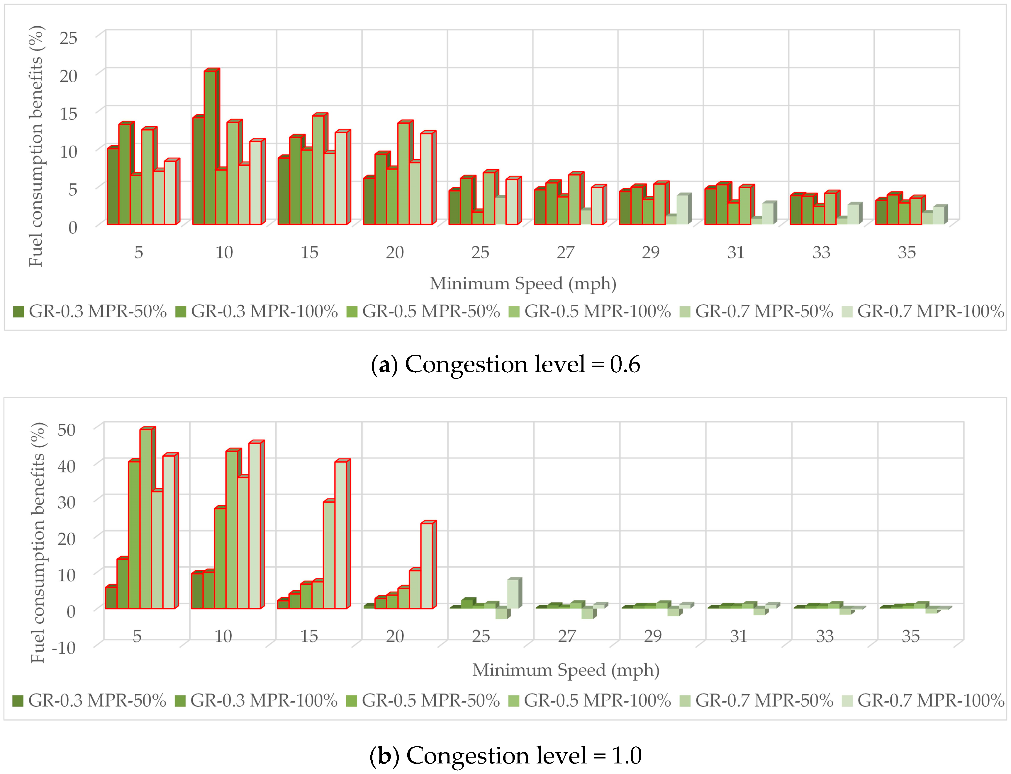
• Few significant throughput benefits were observed. Fuel consumption benefits ranged from 0% to 49.21%. The EAC controller was able to improve the fuel efficiency while it had no adverse effect on the mobility.
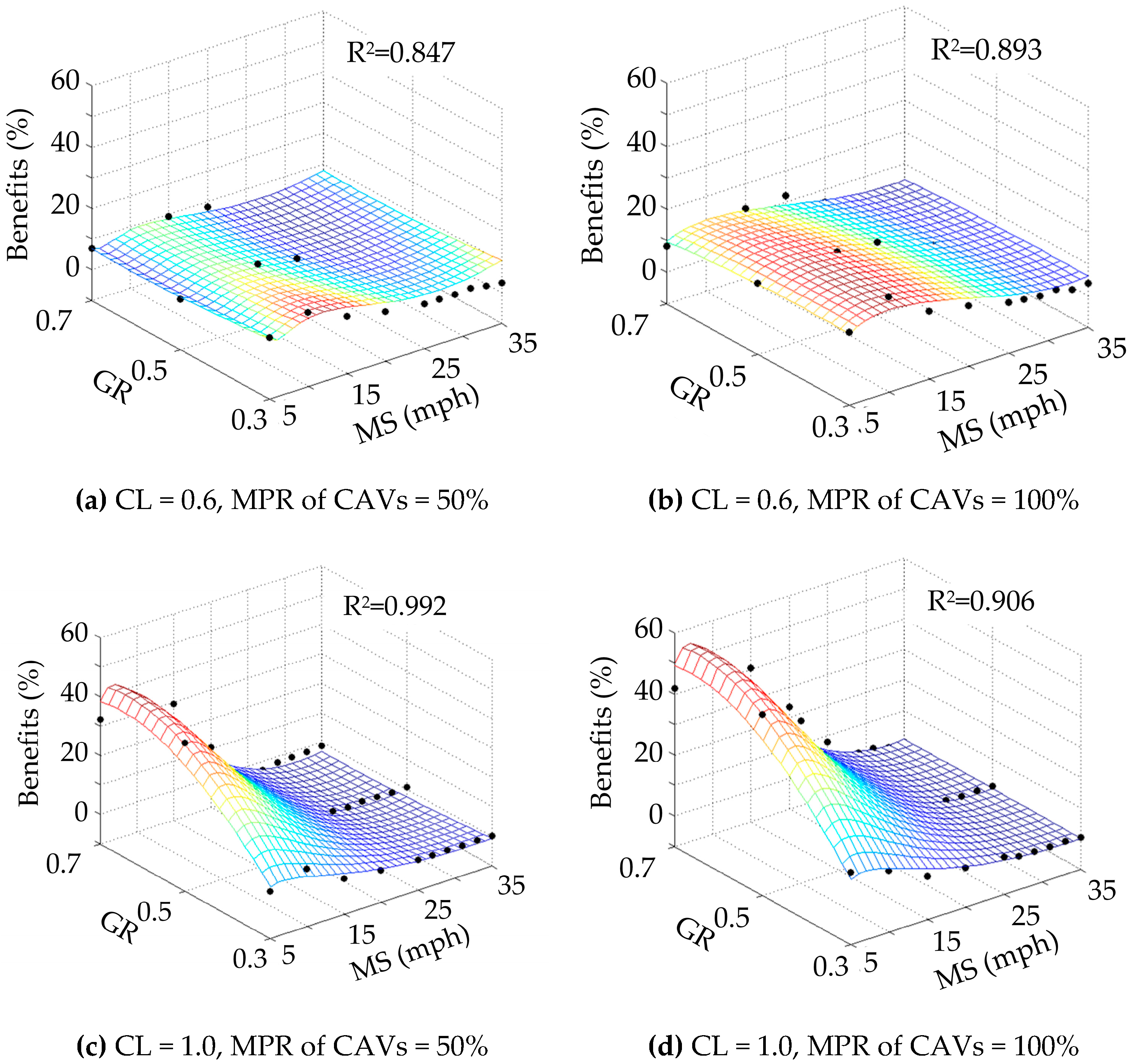
• The fuel consumption benefits were correlated with the percentage of Eco-CAVs and decreased as the MS increased. No significant fuel consumption benefit was generated under a high CL when the MS was greater than 20 mph due to the low percentage of Eco-CAVs. Future installations of EAC control should avoid high MS levels to ensure a high percentage of Eco-CAVs so as to generate significant fuel consumption benefits under various conditions.
• The fuel consumption benefits increased with the MPR of CAVs.
• GR and CL had complex effects on the environmental performance of the EAC controller. The overall trend was that high GR could usually bring high environmental benefits under different CLs.

The evaluation of EAC controller on the corridor showed the following:

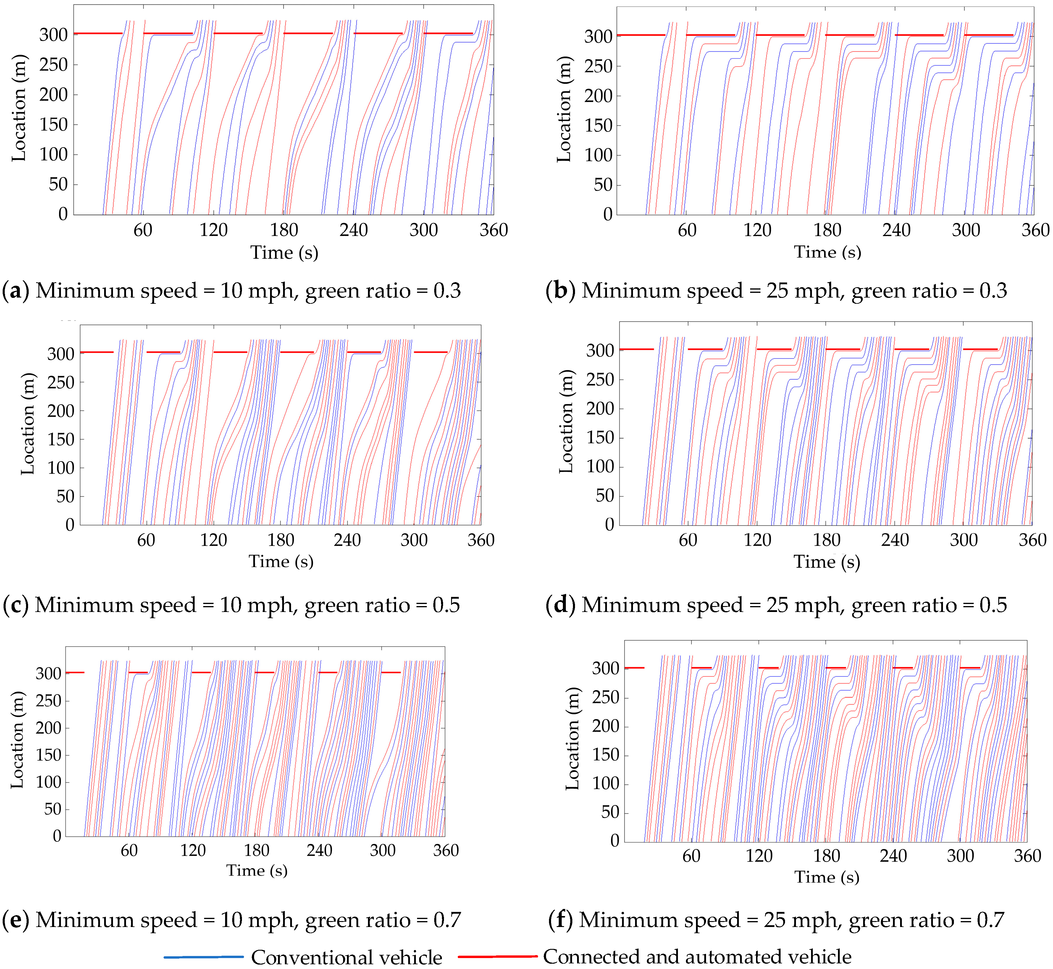
• All the vehicles were clustered into tight marching platoons by the upstream intersection. Significant shockwaves were caused by the deceleration of Eco-CAVs and spread backward in the platoons.
• A significant gating effect occurred when the shockwaves spread in some platoons passed the upstream intersection. It reduced the throughput of the corridor. The EAC controller had no adverse effect on the mobility without this gating effect. Future installations of EAC control should provide enough spread space between the loop detector and upstream intersection for shockwaves to avoid this gating effect.
• Fuel consumption benefits ranged from 0% to 39.86%. The EAC controller was shown to improve the fuel efficiency and reduce emissions under various traffic conditions.
• The fuel consumption benefits increased with the MPR of CAVs. The GR and offset of signal control worked together to affect the percentage of vehicles that could approach and pass through the downstream intersection without great speed adjustments; the fuel consumption benefits decreased with the increase of such vehicles. The EAC controller was found to be more suitable for implementation on the corridor without coordination control.
• The DTI had no direct correlation with the mobility and environmental performance of the EAC controller. However, it was able to restrict the installation location of the loop detector and then indirectly impacted on the performance of EAC controller. The approaching distance from the loop detector to the downstream intersection and the spread space for shockwaves from the loop detector to the upstream intersection affected the environmental performance and mobility performance of the EAC controller on the corridor, respectively.

Overall, the EAC controller was designed for an isolated intersection under low MS levels [16]. There were some performance and function problems when it was implemented in complex road networks. To ensure that this eco-approach control system can be generally applied to various road networks, further improvements should focus on the following two aspects: First, the speed trajectories of CAVs and signal timing plan of intersection should be optimized coordinately to generate non-conflict eco-approach speed trajectories for CAVs under high MS levels. This improvement would reduce the speed adjustment range of CAVs to avoid collisions between the CAV and its following conventional vehicle so as to enhance the environmental and safety performance of the EAC controller. Second, the control strategy of the EAC controller should be improved to delay the deceleration of CAVs when the EAC system is implemented on the corridor under high congestion levels. This improvement could reduce or avoid the gating effect at the upstream intersection to increase the throughput of the corridor with limited space between the loop detector and upstream intersection. It is necessary to construct a new optimization model to balance the improvements in fuel efficiency and emission reduction and the increase in the corridor throughput caused by the delay of CAV deceleration based on the requirements.

In addition, this research did not examine the performance of the EAC controller in multi-lane road networks. A detailed evaluation with explicit consideration of weaving and lane changing maneuvers is also recommended in further research.

References

1. U.S. Environmental Protection Agency. Sources of Greenhouse Gas Emission. 2017. Available online: https://www3.epa.gov/climatechange/ghgemissions/sources/transportation.html (accessed on 25 April 2016).
2. Wu, G.; Boriboonsomsin, K.; Zhang, W.; Li, M.; Barth, M. Energy and emission benefit comparison of stationary and in-vehicle advanced driving alert systems. Transp. Res. Rec. 2010, 2189, 98–106. [Google Scholar] [CrossRef]
3. Qi, X.; Barth, M.; Wu, G.; Boriboonsomsin, K.; Wang, P. Energy impact of connected eco-driving on electric vehicles. In Road Vehicle Automation; Springer: Cham, Switzerland, 2018; Volume 4, pp. 97–111. [Google Scholar] [CrossRef]
4. Hu, J.; Fontaine, D.; Park, B.B.; Ma, J. Field Evaluations of an Adaptive Traffic Signal—Using Private-Sector Probe Data. J. Transp. Eng. 2015, 142, 1–9. [Google Scholar] [CrossRef]
5. Barth, M.; Mandava, S.; Boriboonsomsin, K.; Xia, H. Dynamic ECO-driving for arterial corridors. In Proceedings of the 2011 IEEE Forum on Integrated and Sustainable Transportation System, Vienna, Austria, 29 June–1 July 2011; IEEE: New York, NY, USA, 2011; pp. 182–188. [Google Scholar] [CrossRef]
6. Rakha, H.; Kamalanathsharma, R.K. Eco-driving at signalized intersections using V2I communication. In Proceedings of the 2011 14th International IEEE Conference on Intelligent Transportation Systems, Washington, DC, USA, 5–7 October 2011; IEEE: New York, NY, USA, 2011; pp. 341–346. [Google Scholar] [CrossRef]
7. Wang, M.; Daamen, W.; Hoogendoorn, S.P.; Van Arem, B. Rolling horizon control framework for driver assistance systems. Part I: Mathematical formulation and non-cooperative systems. Transp. Res. Part C Emerg. Technol. 2014, 40, 271–289. [Google Scholar] [CrossRef]
8. Wang, M.; Daamen, W.; Hoogendoorn, S.P.; Van Arem, B. Rolling horizon control framework for driver assistance systems. Part II: Cooperative sensing and cooperative control. Transp. Res. Part C Emerg. Technol. 2014, 40, 290–311. [Google Scholar] [CrossRef]
9. Hu, J.; Shao, Y.; Sun, Z.; Wang, M.; Bared, J.; Huang, P. Integrated optimal eco-driving on rolling terrain for hybrid electric vehicle with vehicle-infrastructure communication. Transp. Res. Part C Emerg. Technol. 2016, 68, 228–244. [Google Scholar] [CrossRef]
10. Ma, J.; Li, X.; Zhou, F.; Hu, J.; Park, B.B. Parsimonious shooting heuristic for trajectory design of connected automated traffic part II: Computational issues and optimization. Transp. Res. Part B Meth. 2017, 95, 421–441. [Google Scholar] [CrossRef]
11. Wang, Z.; Wu, G.; Hao, P.; Boriboonsomsin, K.; Barth, M. Developing a platoon-wide eco-cooperative adaptive cruise control (CACC) system. In Proceedings of the 2017 IEEE Intelligent Vehicles Symposium, Redondo Beach, CA, USA, 11–14 June 2017; IEEE: New York, NY, USA, 2017; pp. 1256–1261. [Google Scholar] [CrossRef]
12. Altan, O.D.; Wu, G.; Barth, M.; Boriboonsomsin, K.; Stark, J.A. GlidePath: Eco-friendly automated approach and departure at signalized intersections. IEEE Trans. Intell. Transp. 2017, 2, 266–277. [Google Scholar] [CrossRef]
13. Xia, H.; Boriboonsomsin, K.; Barth, M. Indirect network-wide energy/emissions benefits from dynamic eco-driving on signalized corridors. In Proceedings of the 2011 14th International IEEE Conference on Intelligent Transportation Systems, Washington, DC, USA, 5–7 October 2011; IEEE: New York, NY, USA, 2011; pp. 329–334. [Google Scholar] [CrossRef]
14. Xia, H.; Boriboonsomsin, K.; Schweizer, F.; Winckler, A.; Zhou, K.; Zhang, W.B.; Matthew, B. Field operational testing of eco-approach technology at a fixed-time signalized intersection. In Proceedings of the 2012 15th International IEEE Conference on Intelligent Transportation Systems, Anchorage Alaska, AK, USA, 16–19 September 2012; IEEE: New York, NY, USA, 2012; pp. 188–193. [Google Scholar] [CrossRef]
15. Hao, P.; Wu, G.; Boriboonsomsin, K.; Barth, M. Developing a framework of eco-approach and departure application for actuated signal control. In Proceedings of the 2015 IEEE Intelligent Vehicles Symposium, Seoul, Korea, 28 June–1 July 2015; IEEE: New York, NY, USA, 2015; pp. 796–801. [Google Scholar] [CrossRef]
16. Jiang, H.; Hu, J.; An, S.; Wang, M.; Park, B.B. Eco approaching at an isolated signalized intersection under partially connected and automated vehicles environment. Transp. Res. Part C Emerg. Technol. 2017, 79, 290–307. [Google Scholar] [CrossRef]
17. Jiang, H.; An, S.; Wang, J.; Cui, J. Eco-approach and departure system for left-turn vehicles at a fixed-time signalized intersection. Sustainability 2018, 10, 273. [Google Scholar] [CrossRef]
18. Ye, F.; Hao, P.; Qi, X.; Wu, G. Prediction-based eco-approach and departure at signalized intersections with speed forecasting on preceding vehicles. IEEE Trans. Intell. Transp. 2018, 20, 1378–1389. [Google Scholar] [CrossRef]
19. Wang, Z.; Wu, G.; Barth, M.J. Cooperative Eco-Driving at Signalized Intersections in a Partially Connected and Automated Vehicle Environment. IEEE Trans. Intell. Transp. 2019, in press. [Google Scholar] [CrossRef]
20. Shao, Y.; Sun, Z. Optimal eco-approach control with traffic prediction for connected vehicles. In Proceedings of the ASME 2018 Dynamic Systems and Control Conference, Atlanta, GA, USA, 30 September–3 October 2018; American Society of Mechanical Engineers: New York, NY, USA, 2018. V002T22A002. [Google Scholar] [CrossRef]
21. Wei, Z.; Hao, P.; Barth, M. Developing an Adaptive Strategy for Connected Eco-Driving under Uncertain Traffic Condition. In Proceedings of the 2019 IEEE Intelligent Vehicles Symposium, Paris, France, 9–12 June 2019; IEEE: New York, NY, USA, 2019; pp. 2066–2071. [Google Scholar] [CrossRef]
22. Williams, N.; Wu, G.; Closas, P. Impact of positioning uncertainty on eco-approach and departure of connected and automated vehicles. In Proceedings of the 2018 IEEE/ION Position, Location and Navigation Symposium (PLANS), Monterey, CA, USA, 23–26 April 2018; IEEE: New York, NY, USA, 2018; pp. 1081–1087. [Google Scholar] [CrossRef]
23. Oh, G.; Peng, H. Eco-driving at signalized intersections: What is possible in the real-world? In Proceedings of the 21st International Conference on Intelligent Transportation Systems (ITSC), Hawaii, HI, USA, 4–7 November 2018; IEEE: New York, NY, USA, 2018; pp. 3674–3679. [Google Scholar] [CrossRef]
24. Cui, L.; Jiang, H.; Park, B.B.; Byon, Y.J.; Hu, J. Impact of automated vehicle eco-approach on human-driven vehicles. IEEE Access. 2018, 6, 62128–62135. [Google Scholar] [CrossRef]
25. Li, W.; Wu, G.; Zhang, Y.; Barth, M. Safety analysis of the eco-approach and departure application at a signalized corridor. Tsinghua Sci. Technol. 2018, 23, 157–171. [Google Scholar] [CrossRef]
26. Xia, H. Eco-approach and Departure Techniques for Connected Vehicles at Signalized Traffic Intersections. Ph.D. Thesis, UC Riverside, Riverside, CA, USA, 25 April 2016. [Google Scholar]
27. Lee, J.; Park, B.B. Development and evaluation of a cooperative vehicle intersection control algorithm under the connected vehicles. IEEE Trans. Intell. Transp. Syst. 2012, 13, 81–90. [Google Scholar] [CrossRef]
28. Almannaa, M.H.; Chen, H.; Rakha, H.A.; Loulizi, A.; Elshawarby, I. Field implementation and testing of an automated eco-cooperative adaptive cruise control system in the vicinity of signalized intersections. Transp. Res. Part D Transp. Environ. 2019, 67, 244–262. [Google Scholar] [CrossRef]
29. Ko, B.; Choi, S.; Park, B.B.; Son, S.H. Field Implementation of Eco-driving and Eco-signal System. In Proceedings of the 3rd International Conference on Vehicle Technology and Intelligent Transport Systems, Porto, Portugal, 23–24 April 2017; Springer: Cham, Switzerland, 2017; pp. 285–292. [Google Scholar] [CrossRef]
30. Hao, P.; Wu, G.; Boriboonsomsin, K.; Barth, M. Eco-approach and departure (EAD) application for actuated signals in real-world traffic. IEEE Trans. Intell. Transp. 2018, 20, 30–40. [Google Scholar] [CrossRef]
31. Lu, S.; Xue, F.; Ting, T.O.; Du, Y. Speed trajectory optimization for electric vehicles in eco-approach and departure using linear programming. In Proceedings of the IET International Conference on Intelligent and Connected Vehicles, Chongqing, China, 22–23 September 2016; IET: Stevenage, UK, 2016; pp. 12–16. [Google Scholar] [CrossRef]
32. Ng, F.; Harding, J.A.; Glass, J. An eco-approach to optimize efficiency and productivity of a hydraulic excavator. J. Clean. Prod. 2016, 112, 3966–3976. [Google Scholar] [CrossRef]
33. Wang, Z.; Wu, G.; Hao, P.; Barth, M. Cluster-wise cooperative eco-approach and departure application for connected and automated vehicles along signalized arterials. IEEE Trans. Intell. Transp. 2018, 3, 404–413. [Google Scholar] [CrossRef] [Green Version]
34. Wang, Z.; Wu, G.; Hao, P.; Barth, M. Cluster-wise cooperative eco-approach and departure application along signalized arterials. In Proceedings of the 2017 20th International Conference on Intelligent Transportation Systems (ITSC), Yokohama, Japan, 16–19 October 2017; IEEE: New York, NY, USA, 2017; pp. 145–150. [Google Scholar] [CrossRef]
35. Li, W.; Wu, G.; Barth, M.; Zhang, Y. Safety, mobility and environmental sustainability of eco-approach and departure application at signalized intersections: A simulation study. In Proceedings of the 2016 IEEE Intelligent Vehicles Symposium, Gothenburg, Sweden, 19–22 June 2016; IEEE: New York, NY, USA, 2016; pp. 1109–1114. [Google Scholar] [CrossRef]
36. Akcelik, R. Efficiency and drag in the power-based model of fuel consumption. Transp. Res. Part B Methodol. 1989, 23, 376–385. [Google Scholar] [CrossRef]
37. Newell, G.F. A simplified car-following theory: A lower order model. Trans. Res. Part B Methodol. 2002, 36, 195–205. [Google Scholar] [CrossRef]
38. Li, M.; Wu, X.; He, X.; Yu, G.; Wang, Y. An eco-driving system for electric vehicles with signal control under v2x environment. Transp. Res. Part C Emerg. Technol. 2018, 93, 335–350. [Google Scholar] [CrossRef]
Figure 1. Control structure of the eco-approach control system. CAVs: connected and automated vehicles.
Sustainability 11 06319 g001
Figure 2. Test road networks. DTI: distance between two adjacent intersections.
Sustainability 11 06319 g002
Figure 3. Improvements of the throughput of an isolated signalized intersection. GR: green ratio, MPR: market penetration rate.
Sustainability 11 06319 g003
Figure 4. Improvements in fuel efficiency of an isolated signalized intersection. GR: green ratio, MPR: market penetration rate.
Sustainability 11 06319 g004
Figure 5. Percentage of CAVs controlled by the eco-approach controller (EAC) controller. GR: green ratio, MPR: market penetration rate.
Sustainability 11 06319 g005
Figure 6. Spatial-temporal trajectories at baseline (CL = 1.0, MPR of CAVs = 0%).
Sustainability 11 06319 g006
Figure 7. Spatial-temporal trajectories of eco-approach control (CL = 1.0, MPR of CAVs = 50%).
Sustainability 11 06319 g007
Figure 8. Fitting surface of fuel consumption benefits. CL: congestion level, MPR: market penetration rate.
Sustainability 11 06319 g008
Figure 9. Optimization results of the optimal controller (L = 300 m). MS: minimum speed.
Sustainability 11 06319 g009
Figure 10. Improvements of the throughput of the corridor. DTI: distance between two adjacent intersections.
Sustainability 11 06319 g010
Figure 11. Improvements of fuel efficiency of corridor. DTI: distance between two adjacent intersections.
Sustainability 11 06319 g011
Figure 12. Spatial-temporal trajectories of eco-approach control (DTI = 320 m, CL = 1.0, MPR = 50%).
Sustainability 11 06319 g012
Figure 13. Spatial-temporal trajectories of eco-approach control (DTI = 600 m, CL = 1.0, MPR = 50%)
Sustainability 11 06319 g013