Efficient Energy-Management System Using A Hybrid Transactive-Model Predictive Control Mechanism for Prosumer-Centric Networked Microgrids

Abstract

With the development of distributed energy resources (DERs) and advancements in technology, microgrids (MGs) appear primed to become an even more integral part of the future distribution grid. In order to transition to the smart grid of the future, MGs must be properly managed and controlled. This paper proposes a microgrid energy management system (MGEMS) based on a hybrid control algorithm that combines Transactive Control (TC) and Model Predictive Control (MPC) for an efficient management of DERs in prosumer-centric networked MGs. A locally installed home energy management system (HEMS) determines a charge schedule for the battery electric vehicle (BEV) and a charge–discharge schedule for the solar photovoltaic (PV) and battery energy storage system (BESS) to reduce residential customers’ operation cost and to improve their overall savings. The proposed networked MGEMS strategy was implemented in IEEE 33-bus test system and evaluated under different BEV and PV-BESS penetration scenarios to study the potential impact that large amounts of BEV and PV-BESS systems can have on the distribution system and how different pricing mechanisms can mitigate these impacts. Test results indicate that our proposed MGEMS strategy shows potential to reduce peak load and power losses as well as to enhance customers’ savings.

1. Introduction

Over the past years, technological developments have driven an increase in distributed energy resources (DERs) across the distribution network, particularly at the demand side. DERs are changing the electrical landscape from a conventional demand-driven power grid to a transactive supply following energy system, where customers (as electricity consumers and/or producers) are actively engaged in transactions and participate in the operation and management of the power grid [1,2,3]. Although the overall installed capacity of DERs is still significantly low, projections indicate a ramp-up in the coming years. According to the U.S. Energy Information Administration (EIA), solar photovoltaic (PV) generation at the distribution level (utility-scale and small-scale) has grown 232% over the past five years (2014–2018), going from a total net generation of 28,925 MWh in 2014 to 96,147 MWh in 2018 [4]. Moreover, the EIA in its 2019 annual energy outlook projects that electricity generation from solar PV will reach 15% of total U.S. electricity generation by 2050 [5].

On another front, transportation has also been experiencing important changes around the world. According to the international energy agency (IEA), in 2017, a new milestone was reached with more than 3 million battery electric vehicles (BEVs) on the road worldwide [6]. Furthermore, the same report projects the worldwide BEV fleet to reach 13 million and 130 million by 2020 and 2030, respectively. Thus, it can be seen that, in the next few years, the increase in BEVs and solar PV generation will cause various integration challenges on the electric grid. The current power grid was not designed to host the increase of load caused by BEV charging and power-flow fluctuations caused by solar PV generation, especially low-voltage distribution networks.

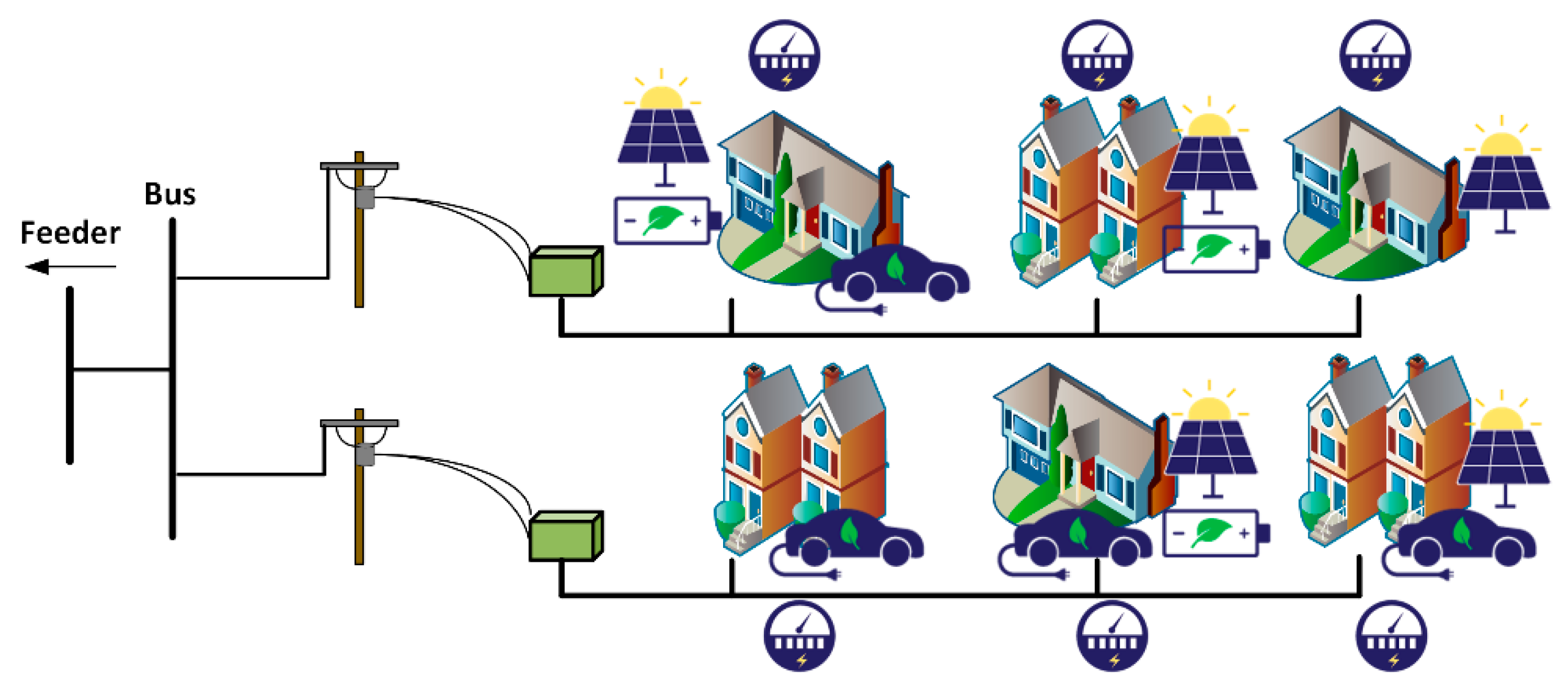
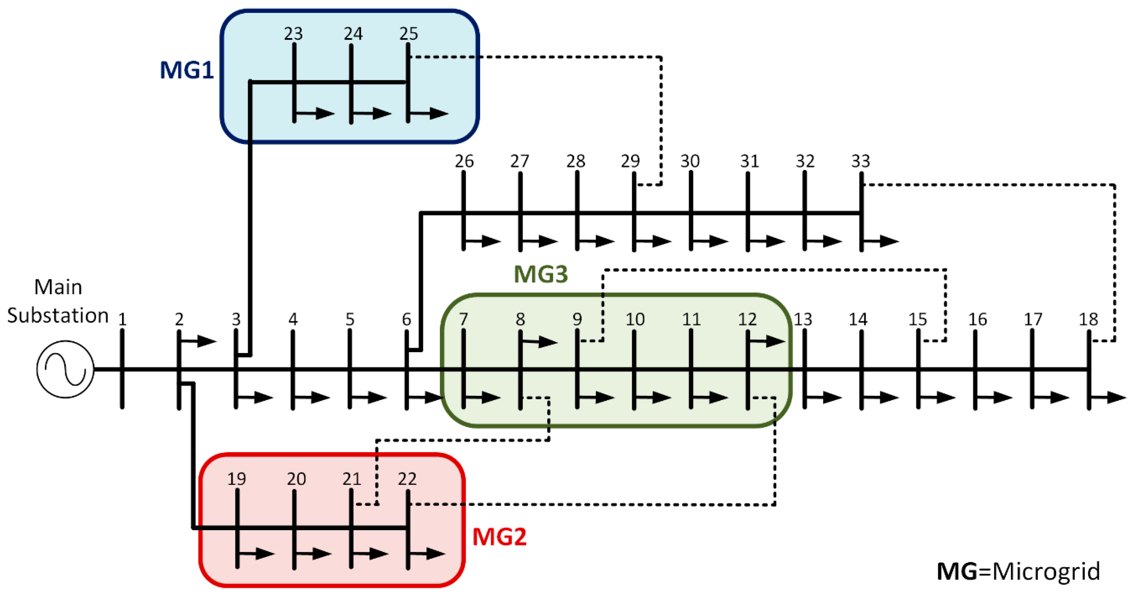
In this regard, Microgrids (MGs), as shown in Figure 1, are considered a key asset of the power grid of the future as they can be used to manage the increasing levels of DERs [7]. MGs are autonomously managed and powered sections of the electrical distribution grid that can be as small as a single building or as large as a downtown area or neighborhood. MGs equipped with advanced communication and control technology can enable coordination between the distribution system and other MGs. Networking of multiple MGs (networked MGs), also known as community MGs, MG cluster, or MG clustering, share a common geographic region and can provide a variety of benefits, e.g., increased efficiency, reliability, and resiliency. Moreover, in the future smart grid, networked MGs could help mitigate the variability of DERs and allow consumers and prosumers to transact and exchange energy (i) among each other and (ii) with other MGs and (iii) to participate in a local retail market providing ancillary services with the rest of the distribution system [8].

Different approaches are proposed in the existing literature to manage and control networked MGs [9,10,11,12,13,14,15,16,17,18]. The role of networked MGs as distributed energy systems to improve power-grid resiliency during extreme weather events is analyzed in Reference [9]. In Reference [10], a multilayered control architecture based on a large-signal model has been proposed to regulate voltage magnitude and frequency as well as output power of DERs within networked MGs. Primary frequency control to support switching transients for networked MGs is reported in Reference [11]. A method for energy-storage dispatch and renewable energy resource sharing in a network of grid-connected MGs to reduce electricity costs is presented in Reference [12]. Shi et al. [13] proposed a distributed energy management strategy formulated as an optimal power-flow problem for the optimal operation of MGs with consideration of the distribution network and the associated constraints. A priority-based energy scheduling mechanism for distribution networks with multiple MGs is described in Reference [14]. Gregoratti and Matamoros [15] addressed a multiple-MG energy-trading strategy in order to minimize the global operation cost while satisfying local energy demand of MGs. A most valuable player algorithm is presented in Reference [16] to optimize the scheduling of the generation units and battery storage of an MG. In Reference [17], a distribution grid service market is proposed to provide voltage stability services in MGs. A demand-side management scheme for cost minimization in a residential MG using strawberry and cuckoo search algorithms is discussed in Reference [18].

Although network-MG control and management has been widely studied [7,8,9,10,11,12,13,14,15,16,17,18], many of these studies fail to analyze the impacts that these approaches might have on conventional distribution networks. As in some cases, the distribution network is not considered [12,15] and in other cases, a simplified version is considered [10,11,13,14]. Thus, some of the solutions obtained from the aforementioned algorithms might be infeasible in practice. Also, most of these studies fail to consider customer willingness to participate in their control strategies, assuming customer participation as a given, i.e., no incentives are offered for customer participation. A transactive control (TC) approach can be used to incentivize customer participation and to help manage DERs in an MG.

A TC is a market-based distributed mechanism that can combine multiple objectives and constraints using uniform transactive incentive signals (TIS) and transactive feedback signals (TFS) [1]. These signals propagate through a communication network where the TC is embedded in the electrical network. TIS and TFS are two different signals with TIS representing the actual delivered cost of electric energy ($/kWh) and TFS dealing with the net electric load (kW) at a specific system location. In recent years, TC-mechanism use in smart grids and MG applications has been studied due to its potential for an efficient DER management and the creation of opportunities to engage in transactions between the different entities that constitute the electrical distribution system, e.g., electric utility and customers. A review of the state-of-the-art of transactive energy systems and concepts are presented in Reference [19]. The potential benefits of TCs were reported in the Pacific Northwest Smart Grid Demonstration project, where the TCs were functional and operational in a variety of pilot projects ranging from MG applications up to wholesale market level transactions [20]. In Reference [21], a transactive bilateral energy-trading mechanism is proposed to minimize the costs for individual participants and to ensure the reliability and security of the distribution system, where Nash bargaining theory and alternating direction method of multipliers (ADMM) are used to model the problem. A multi-agent transactive energy-management framework for networked MGs is presented in [22]. The multi-agent system manages energy imbalances in the MGs, using demand response and battery energy storage systems (BESS) with the objective of minimizing the costs for MG customers. A multi-agent system is also proposed in Reference [23], where an auction-based locational marginal price (LMP) is used to motivate the energy transactions among MGs. In Reference [24], a day-ahead transactive market framework is proposed for DER scheduling to reduce local supply costs. TCs are used for BEV charging in References [25,26,27]. A TC based on model predictive control (MPC) is used for real-time scheduling of BEVs in Reference [25], where the MPC is used to clear a day-ahead transactive market. In Reference [26], the charging demand of the BEV is used to manage uncertainties of the building PV generation. Hu et al. [27] implemented a TC with the purpose of minimizing the BEV-charging cost as well as of preventing grid congestion and voltage violations. A reactive power incentive program to maintain distribution-system reliability is presented in Reference [28]. In Reference [29], a Nash bargaining formulation is proposed for energy trading between networked MGs for MG operation cost reduction. A TC coupled with a pricing rule is proposed for grid-connected, islanded, and congested networked MGs in Reference [30]. DC MGs have also been studied for application of TCs [31,32,33]. In Reference [31], a framework is proposed for short-term operation of DERs, controllable demands, and MGs in a transactive energy architecture, with a focus on the distributed energy management of hybrid AC/DC microgrids. Jingpeng et al. [32] presented a centralized energy-management system approach based on transactive energy to reduce the total operation cost and to achieve efficiency in a DC residential system. In Reference [33], a transactive energy-management system for supply/demand coordination with demand response programs was implemented to manage rural DC MGs.

Several other models have been proposed for BEV charging/discharging and pricing scheduling [34,35,36,37,38,39]. The impact of variable prices on the behavior of BEV users is studied in Reference [34], where the variable prices are determined based on the calculation of distribution locational marginal price (DLMP) and updated continuously based on the users’ trips and behavior. In Reference [35], an optimal Time-of-Use (TOU) schedule and a controlled BEV-charging algorithm are used to maximize both customer and utility benefits, and a controlled charging algorithm is also proposed to improve thier voltage quality at the EV load locations while avoiding customer inconvenience. In Reference [36], meta-heuristic techniques are used for charging coordination of BEVs with simultaneous operation of capacitor switching to minimize power losses and voltage deviation in a distribution system. Furthermore, a TOU electricity tariff was included in the proposed charging coordination to reduce the PEV charging cost. Cherikad et al. [37] proposed a distributed dynamic pricing model for BEV-charging and -discharging scheduling and building energy management in an MG. Their model consisted of a cloud-software defined networking communication architecture and a linear optimization approach to achieve efficiency in the MG. Pasetti et al. [38] proposed a model to estimate the price of BEV charging considering the impacts solar PV generation has on the charging costs of BEVs. The model estimated the costs considering demand charges and utility loss of revenue and was compared to a TOU tariff. In Reference [39], a two-stage real-time optimization algorithm is proposed to recharge a fleet of plug-in BEVs to minimize costs, to avoid creating new peaks in the demand profile, and to improve use of power system equipment. The optimization algorithm used a dynamic price signal based on probabilistic models developed using historical price data.

Motivated by the promising benefits of using TCs, this paper proposes a hybrid control mechanism based on the combination of TC and MPC for an efficient management of DERs in prosumer-centric networked MGs. Hereinafter, the proposed control approach is termed TC+MPC. This paper further presents a detailed analysis of the impacts (economical and technical) produced by the TC+MPC within the MGs, and the distribution system as a whole is presented. To carry out this analysis, a Monte Carlo Simulation (MCS) is proposed to consider BEV driving uncertainties and the proposed hybrid TC+MPC management system is used to manage DERs. The hybrid TC+MPC combines the control capabilities and features of the MPC with the TIS–TFS signals of the TC, creating a robust control mechanism that is driven by price signals. The objective of the TC+MPC management system is to produce optimal BEV charge and solar PV-BESS charge/discharge schedules to significantly reduce the residential MG customers’ operational cost and to improve their overall savings. The proposed MG energy-management system (MGEMS) is evaluated considering different case studies and scenarios to analyze the impacts that BEV and PV-BESS systems can have on the distribution network.

To the best knowledge of the authors, the proposed hybrid control mechanism, i.e., TC combined with MPC and MCS, has not been applied in the area of networked microgrid energy-management systems, thereby advancing the state-of-the-art in controlling mechanisms for networked MGs. In contrast to the existing literature, the major contributions of this paper to the state-of-the-art are the following:

• Development of a new hybrid TC+MPC control mechanism to manage DERs (BEVs, solar PV, and BESS) of networked MGs constituted by consumer groups (CGs) and prosumer groups (PCGs) and detailed study of their behavior while being incentivized by different price signals;
• Development of TIS and TFS signals, where TIS is based on distribution locational marginal price (DLMP) and distribution system conditions, whereas TFS development is based on CG/PCG net load and BEV driving patterns generated by MCS.
• Detailed analysis of the impacts on the distribution grid due to the use of TCs for DER management, i.e., bus voltage and power loss impacts.
• Detailed cost/savings analysis for consumers/prosumers under different pricing rates when they are equipped with BEVs, solar PV, and hybrid solar PV-BESS systems.

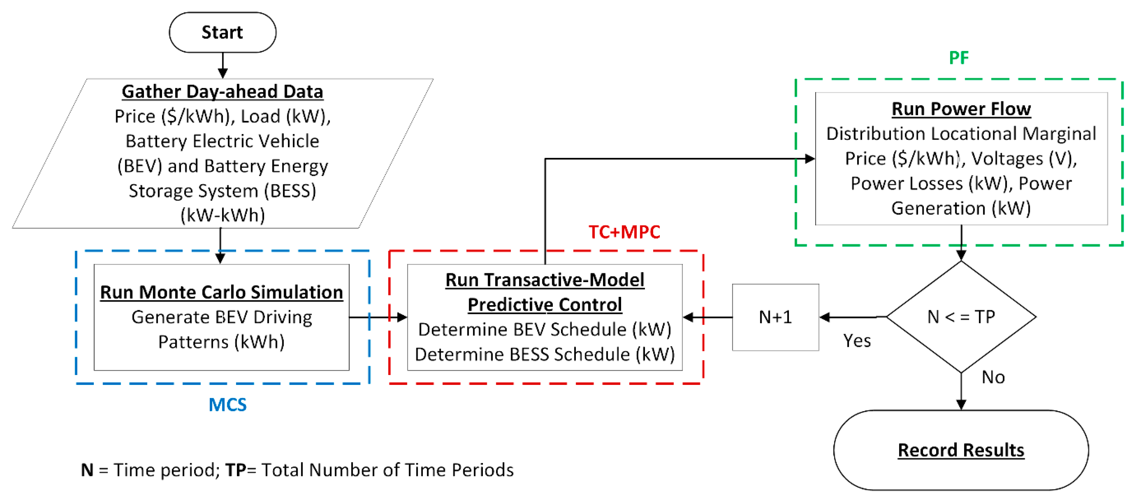
In order to evaluate the proposed TC+MPC based energy-management system, five case studies (with and without PV/BESS and under different price signal scenarios) are conducted on residential networked MGs based on an IEEE 33-bus test system. The remainder of this paper is organized as follows. Section 2 details the essential components of the proposed TC+MPC-based MGEMS with the uncertainty modeling and the incentive signal formulation. Numerical test results and discussion are presented in Section 3, and Section 4 concludes the paper.

2. Transactive Control-Based Microgrid Energy-Management System Formulation

This section describes the detailed TC-based MGEMS formulations and comprises the step-by-step procedures followed by several contextual elements required for the optimization procedure, i.e., MCS, BEV, and BESS modeling for the MPC, and the schedule optimization process.

2.1. Optimization and Control Procedure

The control hierarchy of the distribution system proposed in this paper is considered to be a hybrid control approach, which is divided into centralized and decentralized control mechanisms. The MG controls are assumed to be decentralized as they use the local information (available solar PV power and state of charge of the BEV and BESS) to optimize and coordinate their schedules. A centralized control is assumed to be supervised by the distribution system operator (DSO), ensuring generation–demand balance and providing ancillary services for the whole distribution system.

The initial step is the preparation of the input data, i.e., day-ahead electricity price, residential load, solar PV power output, and BEV driving patterns. The initial step also requires the definition of the technical parameters of the DER considered in the case studies, e.g., BEV and BESS battery capacity and charging limits.

Once the input data is prepared, an MCS is conducted to generate a set of BEV driving patterns. This step is explained in detail in Section 2.2. The following task is to execute a set of TCs based on MPC to determine the charge schedule of the BEVs and the charge/discharge schedule of the BESS. The mathematical models and MPC formulation are presented in Section 2.3. The next task is to assign the load profiles to each bus in the test system and to run a power-flow simulation to calculate the bus voltages, DLMP, power generation, and power losses.

The final step in the procedure is to calculate the costs/savings for the consumers/prosumers, net load, and final BEV and BESS schedules. Figure 2 presents a flow chart of the different steps of the optimization and control procedure.

2.2. Monte Carlo Simulation

MCS is an accurate technique to estimate probability density functions (PDFs) using historical data. In this paper, an MCS is used to generate daily driving patterns of BEVs to represent the stochastic nature of BEV charging. The MCS requires historical BEV driving patterns ($\delta$) to generate a random BEV driving pattern. To consider uncertainties, the underlying stochastic formulation of MCS must include two random components: a uniform distribution ($RU$) and a normal distribution ($RN$). A distribution function to describe the driving behavior of BEV fleets using an MCS was developed in Reference [40]. The distribution function used in Reference [40] has been adopted in this paper and applied in the MCS. The distribution function used to represent the BEV random driving pattern is formulated as follows:

$$d_{n,k}^i=({\delta }_k^i+R{U}_{n,k}^i)\cdot (1+R{N}_{n,k}^i),$$

(1)

where $d_{n,k}^i$ is the stochastic driving pattern of BEV $i$ at time period $k$ and scenario $n$. ${\delta }_k^i$ is the expected energy consumption of BEV $i$ at time period $k$. This process is repeated for a specified number of scenarios $n$ that ensures convergence over a simulation period $t$.

Samples of historical data are used for the MCS and are constituted by BEV driving patterns in terms of BEV battery energy usage [40]. These BEV driving patterns reflect conventional driving by residential customers and are considered as the base driving patterns.

2.3. Transactive-Model Predictve Control Formulation

MPC, also known as Receding Horizon Control (RHC), has been developed considerably over the past years and has widely been recognized for its application in academic research and the industry. MPC is a control methodology that computes an optimal control action based on a model of a dynamic system and its predicted future evolution [41]. The control objective and the mathematical model are formulated as an optimization problem that repeatedly computes the control inputs. The objective can be to maximize profit, to minimize operational costs, or to force a system to follow a predetermined trajectory. Only the computed inputs associated with the current time step are actuated on the physical system. A new current model state is estimated regularly when new measurements are available, and the real-time optimization procedure is repeated.

In this paper, the BEV and BESS batteries are formulated as discrete time space models to be used in an MPC. The discrete state space model is formulated as follows [41]:

$$x_{k+1}=A{x}_k+B{u}_k+E{d}_k\mathrm{k}\in N,$$

(2)

$$y_k=C{x}_k \mathrm{k}\in N,$$

(3)

$$x(0)=x_0,$$

(4)

where $x_k$ is the state at time period $k$, $u_k$ is the input variable, $y_k$ is the output variable, $d_k$ is a random variable acting on the state transition, $A$ is the state transition matrix, $B$ is the input matrix, $E$ is the disturbance matrix, $C$ is the output matrix, and $x_0$ is the initial state. In Equation (2), $u_k$ represents the control variable and the battery state of charge (SOC) is equal to the output variable: $y_k=x_k$ In the case of the BEV model, BEV driving usage is represented by $d_k$ as a disturbance of the battery SOC. When modeling the BESS, $d_k$ represents the residual solar PV power. The BEV daily usage is modeled using BEV driving patterns generated by the MCS. The state space matrices of the model are the following Equations (5)–(8).

$$A=1,$$

(5)

$$B=(\eta /BE{V}_{\max }^{})Ts,$$

(6)

$$C=1,$$

(7)

$$E=-(\eta /BE{V}_{\max }^{})Ts,$$

(8)

where η is the BEV or BESS efficiency, BEV_max is the maximum charging of the BEV or BESS, and $Ts$ is the chosen time sample. The state transition matrix ($A$) and the output matrix ($C$) are set to 1 as it is assumed that no other factors affect the state of charge of the batteries. If other factors were to be considered (e.g., battery degradation and temperature) to affect the state of charge of the batteries, these matrices would be modified. For BESS modeling, matrix $B$ is negative and $E$ is positive. The change in signs of matrices $B$ and $E$ for the BESS model is because the input variable ($u_k$) is now controlling the discharge of the battery (decreasing the SOC of the battery) and the solar PV power ($d_k$) is charging the battery (increasing the SOC of the battery).

2.3.1. Battery Electric Vehicle Schedule Optimization

Adopting the discrete time space model presented in Equations (2)–(8), the optimal BEV charge schedule is achieved while minimizing the charging costs as shown in the objective function of Equation (9), which is subject to constraints of Equations (10)–(13).

$$\min \mathrm{F}={\displaystyle \sum _{k=0}^{N-1}{p}_k\ast (}{u}_{BEV,k}),$$

(9)

$$\begin{array}{l}\mathrm{subject} \mathrm{to} \\ x_{BEV,k+1}=A{x}_{BEV,k}+B{u}_{BEV,k}+E{d}_{BEV,k}k\in N,\end{array}$$

(10)

$$y_{BEV,k}=C{x}_{BEV,k}k\in N,$$

(11)

$$u_{BEV\min }\le u_{BEV,k}\le u_{BEV\max ,k}k\in N,$$

(12)

$$y_{BEV\min }\le y_{BEV,k}\le y_{BEV\max }k\in N,$$

(13)

where, in Equation (9), $N$ is the prediction horizon, $p_k$ is the electricity price, and $u_{BEV,k}$ is the charging power. The discharge constraints are not considered for BEV modelling as the BEV discharge is based on the customer driving patterns and is controlled by the on-board computer of the BEV. From Equation (10), $x_{BEV,k+1}$ is the BEV future SOC; $y_{BEV,k}$ is the current battery SOC; and $u_{BEVmin}$ and $u_{BEV\max ,k}$ are the battery minimum and maximum charging power, respectively. The constraint of Equation (13) represents the minimum and maximum SOC of the battery. The optimal BEV charging plan $u_{BEV,k}$ will be solved for the determined prediction horizon $N$. To carry out the simulations and to determine the optimal charging schedule forecasted, BEV load $d_{BEV,k}$ and electricity price $p_k$ are used.

2.3.2. Battery Energy Storage System Schedule optimization

Similar to the BEV, the BESS is modeled as Equations (2)–(8). The objective function of Equation (14) is to maximize the savings of prosumers by optimizing the BESS discharging schedule subject to the constraints of Equations (14)–(19). The objective function for the MPC can be formulated as follows [42,43]:

$$\max \mathrm{F}={\displaystyle \sum _{k=0}^{N-1}{p}_k\ast (}{u}_{BESS,k}),$$

(14)

$$\begin{array}{l}\mathrm{subject} \mathrm{to} \\ x_{BESS,k+1}=A{x}_{BESS,k}+B{u}_{BESS,k}+E{d}_{BESS,k}k\in N,\end{array}$$

(15)

$$y_{BESS,k}=C{x}_{BESS,k}k\in N,$$

(16)

$$u_{BESS\min }\le u_{BESS,k}\le u_{BESS\max ,k}k\in N,$$

(17)

$$d_{BESS\min }\le d_{BESS,k}\le d_{BESS\max ,k}k\in N,$$

(18)

$$y_{BESS\min }\le y_{BESS,k}\le y_{BESS\max }k\in N,$$

(19)

where $x_{BESS,k+1}$ is the future SOC of the BESS; $y_{BESS,k}$ is the BESS SOC; and $u_{BESSmin}$ and $u_{BESS\max ,k}$ are the BESS minimum and maximum discharging power, respectively. In Equation (18), $d_{BESSmin}$ and $d_{BESS\max ,k}$ are the minimum and maximum charging power of the BESS, respectively, and in Equation (19), $y_{BESSmin}$ and $y_{BESSmax}$ are the minimum and maximum SOC of the BESS, respectively. The optimal BESS discharging plan $u_{BESS,k}$ will also be solved for the determined prediction horizon N. To determine the optimal discharging schedule, forecasted solar PV power ($d_{BESS,k}$) is considered as the disturbance.

2.4. Formulation of Incentive Signals

In this paper, DLMP is considered for energy pricing and used for the TC operation. The DLMPs are determined by minimizing the cost of generation considering the physical constraints of the distribution system, which exposes producers and consumers to the marginal cost of electricity delivery at different locations. The DLMP is constructed based on three components: (i) the wholesale locational marginal price (LMP), (ii) system conditions (available generation, load demand, and losses), and (iii) uplift costs (operation and maintenance costs). The LMP is defined as the marginal increase in the overall system costs for the additional per-unit active power consumption at each transmission bus. For simulation purposes, it is assumed that the DSO receives the LMP, determines the DLMP at each bus of the distribution network for the next day, and updates the DLMP in an hourly manner. Equations (20) and (21) describe the calculations for TIS and TFS, respectively [43]. The TIS is formulated in the following manner:

$$TI{S}_{i,t}=DLM{P}_t+L{C}_t+TOC+LOL{C}_t,$$

(20)

where DLMP_t is the DLMP at time t, LC_t is the cost of distribution losses at time t, TOC is the total owning costs of the transformer, and (LOLC) the penalty cost for transformer loss of life. The estimated transformer TOC considers the initial transformer cost and the cost to operate and maintain the transformer over its life. The transformer LOLC is estimated based on the loading of the transformer. Similarly, TFS signal represents the net load of the customer and is calculated as follows:

$$TF{S}_{i,t}=D_{i,t}+BEV{L}_{i,t},$$

(21)

where $D_{i,t}$ is the demand of customer i at time t and $BEV{L}_{i,t}$ is the BEV charging demand of customer i at time t.

The TIS and TFS signals are used in the MPC formulations presented in Section 2.3.1 and Section 2.3.2 to create a hybrid TC+MPC mechanism. This is achieved by replacing the electricity price $p_k$ with the TIS and by employing the TFS as a disturbance in the MPC discrete time space models.

3. Numerical Results and Discussion

In this section, case studies are presented to test the proposed hybrid TC+MPC scheduling method on an IEEE 33-bus radial distribution system. For simulation purposes, BEV penetration is considered based on the EV30@30 campaign [44]. The EV30@30 campaign was launched at the Eighth Clean Energy Ministerial in 2017 in which the collective goal for all Electric Vehicle Initiative members is to reach a 30% market share for BEVs by 2030. In the case studies, a total of 242 households are assumed to be located in three MGs. Data from the US Census Bureau [45] was used to estimate the number of households that own vehicles, and assuming a 30% BEV penetration, a fleet of 74 BEVs is considered to be distributed among the households located in each MG. Three BEV historical driving patterns are considered for the case studies [40]. Detailed historical BEV driving data expressed in kWh is shown in

Table A1. Historical BEV daily driving patterns.

BEV Driving Patterns (kWh)
Hour (h)	BEV1	BEV2	BEV3	Hour (h)	BEV1	BEV2	BEV3
1	0.0	0.0	0.0	13	1.6	0.0	0.0
2	0.0	0.0	0.0	14	0.0	0.0	0.0
3	0.0	0.0	0.0	15	0.0	0.0	2.7
4	0.0	0.0	0.0	16	2.7	1.3	2.7
5	0.0	0.0	0.0	17	4.8	1.6	0.0
6	2.7	1.3	2.7	18	3.2	1.6	0.0
7	3.8	1.9	2.7	19	0.0	0.0	0.0
8	4.8	2.4	0.0	20	2.7	0.0	2.7
9	0.0	1.3	0.0	21	3.0	0.0	2.7
10	0.0	0.0	4.0	22	0.0	0.0	0.0
11	0.0	0.0	5.4	23	0.0	0.0	0.0
12	1.6	0.0	0.0	24	0.0	0.0	0.0

in Appendix A. For the simulation, 1000 scenarios are generated for each BEV type.

Table 1. Parameters of random components of residential customer Battery Electric Vehicle (BEV).

	Parameter	Battery Electric Vehicle 1 (BEV1)	Battery Electric Vehicle 2 (BEV2)	Battery Electric Vehicle 3 (BEV3)
	No. of Scenarios	1000	1000	1000
Normal Distribution (RN)	Stand. Dev (kWh)	2	1	2
	Mean (kWh)	1	0.5	1
Uniform Distribution (RU)	(kWh)	0–1	0–1	0–1
Confidence Interval µ	Lower Bound (kWh)	0.5668	0.1471	0.3748
	Upper Bound (kWh)	0116	0.8170	1.7552
Confidence Interval σ	Lower Bound (kWh)	1.3297	0.6166	1.2705
	Upper Bound (kWh)	2.3999	1.1128	2.2930

shows the BEV parameters used to calculate the random components that are needed for generating BEV driving patterns by MCS.

The three MGs considered for the simulations are assumed to be located in a 33-bus radial distribution system, as shown in Figure 3. The test system data was acquired and modified from Reference [46] by placing three MGs along the feeders of the test system and by modifying the load values. Detailed bus load data for the 33-bus distribution system is shown in

Table A2. Load data for the 33-bus distribution system.

Bus	Pd (kW)	Qd (kVAR)	Bus	Pd (kW)	Qd (kVAR)
2	97	60	18	64	40
3	80	40	19	24	40
4	117	80	20	19	40
5	43	30	21	29	40
6	58	20	22	21	40
7	71	100	23	24	50
8	97	100	24	29	200
9	49	20	25	27	200
10	48	20	26	58	25
11	35	30	27	58	25
12	44	35	28	58	20
13	58	35	29	85	70
14	117	80	30	195	600
15	43	10	31	145	70
16	58	20	32	204	100
17	58	20	33	58	40

in Appendix A. In Figure 3, each bus represents a distribution transformer and the dotted lines indicate normally open tie lines. Connected to each transformer are sets of residential customers that are aggregated as CGs or PCGs depending on their classification, i.e., consumer or prosumer. The tie lines are not used in the case studies and are only kept to maintain the test system topology as described in Reference [46].

To run the simulations, actual hourly data of load, PV power output, and electricity price have been used. Price data (fixed and time-of-use rates) were obtained from El Paso Electric, a utility in the U.S. southwest [47,48]. The LMP price data was obtained from Pennsylvania, Jersey, Maryland Power Pool (PJM) market [49]. The load data was obtained from the U.S. 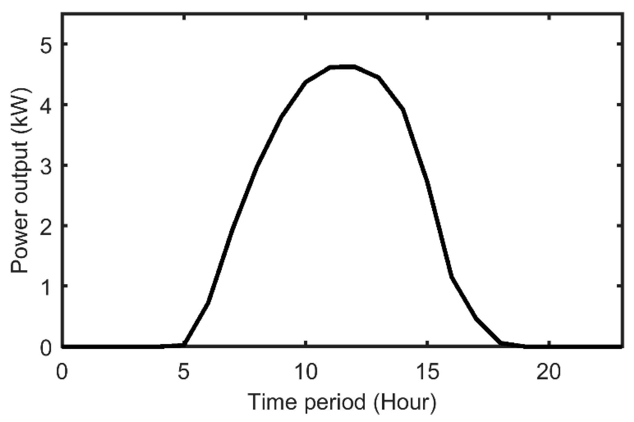Department of Energy Open Data Catalog, residential load at TMY3 locations for the surrounding region of Ashland, Oregon [50]. The specific locations are Klamath Falls, Medford-Rogue Valley, and Redmond, all from Oregon. The solar PV power output data was obtained from a solar PV system located in Ashland, Oregon. The solar PV power output profile is representative of a sunny summer day. Figure 4 shows the solar PV power output profile considered for each prosumer. The load data was selected for these locations to make the simulation more realistic as the PV power output is considered for the same region. Moreover, by using real load, price, and PV data, the case study results can better illustrate the potential benefits that can be achieved by using a TC+MPC for BESS and BEV management in residential networked MGs.

Most of the latest BEV models (2019 and newer) that are being produced have driving ranges above 200 miles and are equipped with batteries that have capacities between 60 kWh and 100 kWh [51]. Furthermore, five of the top ten selling BEVs in the U.S. have battery capacities of 60 kWh or higher [52]. Therefore, it is expected that newer BEV models will continue this trend which will become the norm in most distribution systems in the future. Hence, for BEV modeling, a Tesla Model S is considered [53]. The Model S offers various battery capacity presentations; we considered the 70-kWh battery. It is assumed that the maximum charging power is 10 kW which is based on a 240-V, 40-A connection. A large-scale electric vehicle deployment project known as My Electric Avenue was conducted in the United Kingdom between January 2013 and December 2015 [54] in which one of the major findings was that the likelihood of a BEV being charged when its initial SOC was 16.6% or lower is less than 15%. Another study conducted by the Idaho National Laboratory, U.S.A. found that the average percentage of users who started a commute or a charge with an SOC of 20% or lower is less than 5% [55]. Thus, for simulation purposes, we assume the minimum and maximum BEV SOCs to be 20% and 100%, respectively. The BESS considered for the simulations is a Tesla Powerwall [56]. The PowerWall battery has a capacity of 13.5 kWh and a charging/discharging power of 5 kW. The minimum and maximum BESS SOCs are set as 0% and 100%, respectively. The information regarding the BEVs and BESS is presented in

Table 2. Battery electric vehicle data [53].

Battery Electric Vehicle (BEV) Parameter	Value
BEV battery size	70 kWh
BEV battery efficiency	90%
Maximum charging power	10 kW
Minimum State-of-Charge (SOC)	20%
Maximum State-of-Charge (SOC)	100%

and

Table 3. Battery energy storage system data [56].

Battery Energy Storage System (BESS) Parameter	Value
Energy Capacity	13.5 kWh
Operating Voltage	240 V
Operating Current	48 A
Peak Power	7 kW
Continuous Power	5 kW
Round-Trip Efficiency	90%
Depth of Discharge	100%

, respectively. The data used for the case study is summarized in

Table 4. Case study data.

Prosumer Group (PCG) Consumer Group (CG)	Bus	Households (HHs)	Load (kW)	Solar Photovoltaic (PV) (kW)	BEV (kW)	BESS
						Capacity (kWh)	Output (kW)
Microgrid 1 (MG1)
PCG1	23	10	32	50	60	270	50
PCG2	24	12	34	60	50	324	60
CG1	25	15	42	-	50	-	-
Microgrid 2 (MG2)
PCG3	19	10	28	50	50	270	50
CG2	20	11	30	-	60	-	-
PCG4	21	12	38	60	40	324	60
PCG5	22	12	34	60	30	324	60
Microgrid 3 (MG3)
CG3	7	40	70	-	50	-	-
CG4	8	40	100	-	60	-	-
PCG6	9	20	48	100	70	540	100
PCG7	10	20	48	100	70	540	100
CG5	11	20	35	-	70	-	-
PCG8	12	25	45	125	80	675	125

, where households are abbreviated as HHs, Load represents the peak load, Solar represents the maximum PV power output, BEV represents the peak BEV load, and BESS—Capacity and Output are the BESS storage capacity and rated power output, respectively.

Increasing penetration of DERs is requiring utilities to adjust their current price rates and to design new ones to better align pricing and costs with price signals that guide customer usage [57]. Different utilities in the U.S. already have plans in place and are transitioning their customers from fixed tariffs to TOU tariffs [58]. Thus, we propose to compare three types of price tariffs (fixed, time-of-use, and dynamic) and to analyze the impacts each type has on the customers and on the distribution system. The operation of the proposed TC+MPC was analyzed considering five case studies. The following case studies were tested and compared with the base case and among each other.

Table 5. Case study characteristics.

	Load	BEV	PV	BESS	Price Signal
Case 1	✓	✓			Fixed
Case 2	✓	✓	✓		Fixed
Case 3	✓	✓	✓	✓	Fixed
Case 4	✓	✓	✓	✓	Time-of-Use (TOU)
Case 5	✓	✓	✓	✓	Dynamic Price (DP)

presents a summary of the different case studies.

• Case 1: Considering Load and BEV (Without PV and BESS)—Under Fixed Price Signal Scenario
• Case 2: Considering Load, BEV, and PVs (Without BESS)—Under Fixed Price Signal Scenario
• Case 3: Considering Load, BEV, PV, and BESS—Under Fixed Price Signal Scenario
• Case 4: Considering Load, BEV, PV, and BESS—Under Time of Use price Signal Scenario
• Case 5: Considering Load, BEV, PV, and BESS—Under Dynamic Price Signal Scenario

The base case considers only residential and BEV loads. The base case (Case 1) is similar to current electrical distribution systems throughout the U.S. and around the world. Case 2 is the next step of evolution of the conventional distribution system, where customers also have roof-top solar PV installations. Cases 3–5 assume customers have BESS technology, which enables them to participate in an electricity retail market and to respond to incentive signals generated by the DSO. For all case studies, an individual charge schedule is produced for each BEV. Also, an individual charge/discharge schedule is produced for each BESS. The following assumptions are considered for all case studies:

• The consumers/prosumers are equipped with home energy management system (HEMS), in which the hybrid TC+MPC mechanism is embedded.
• The hybrid TC+MPC mechanism is used for all case studies.
• The BEV charge is analyzed only at the consumer/prosumer household, i.e., charging between 6 am and 6 pm is not available.
• Net metering is considered for cost/savings calculations.
• The BEV SOC must remain at least at 20% throughout the day.
• The BEV cannot be in driving mode (discharging) and charging mode simultaneously.
• The BESS cannot be charged/discharged simultaneously.

3.1. Case 3: Fixed Price Signal Scenario

In this case, a fixed cost is used [47]. This case can be considered the conventional case as most residential customers around the world pay the electric utility or DSO at a fixed rate for electricity. In the US, normally, it is expressed in dollars per kilowatt-hour ($/kWh). Under this pricing rate, there is no incentive for customers who own BEVs to charge at different times, e.g., during off-peak hours. Thus, BEV charging is uncontrolled and BEVs are charged at any time. In the case of customers that own PV-BESS systems, the BESS discharge is also uncontrolled and can be discharged at any time as there is no incentive to discharge, for example, during peak load hours. 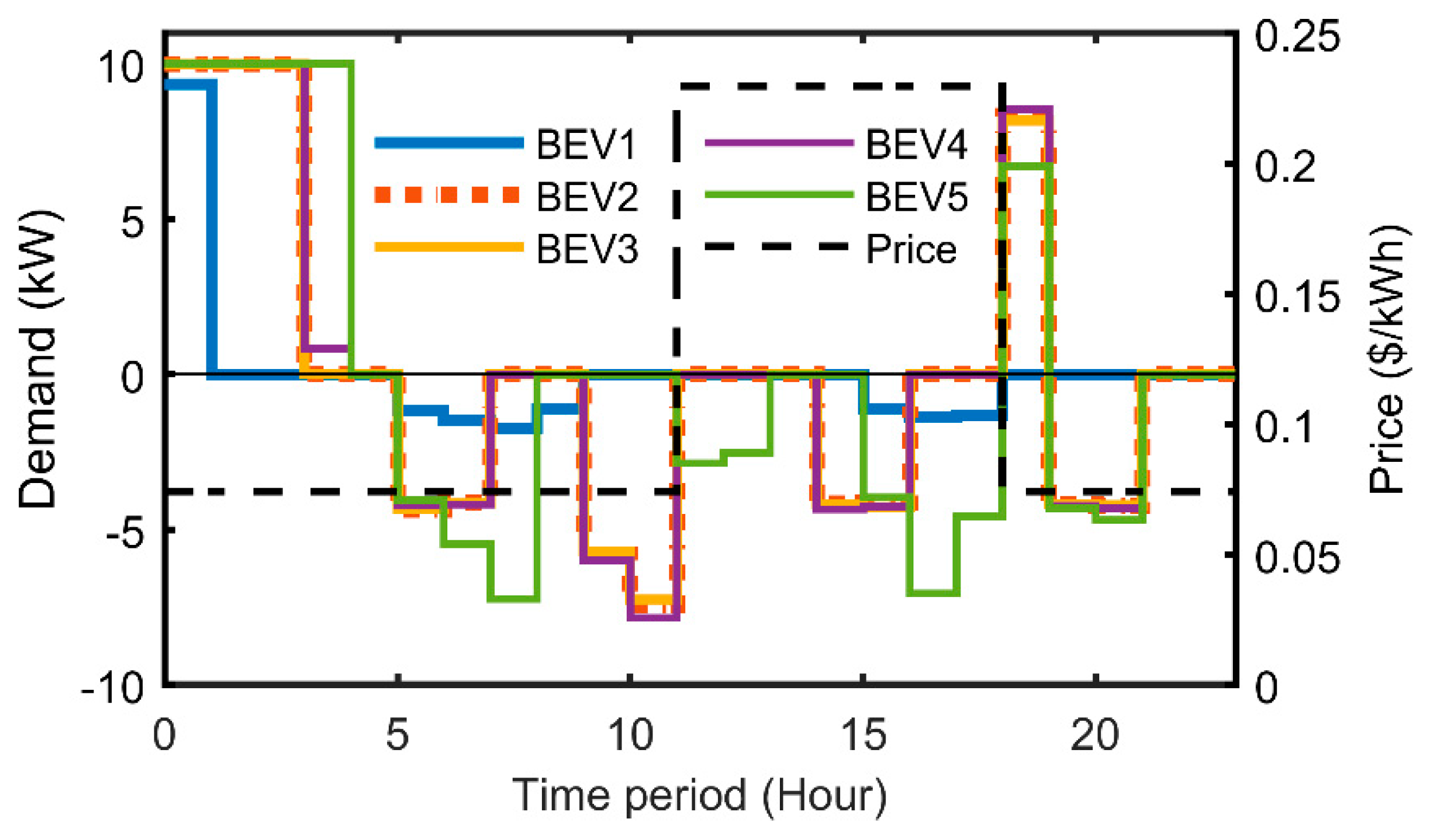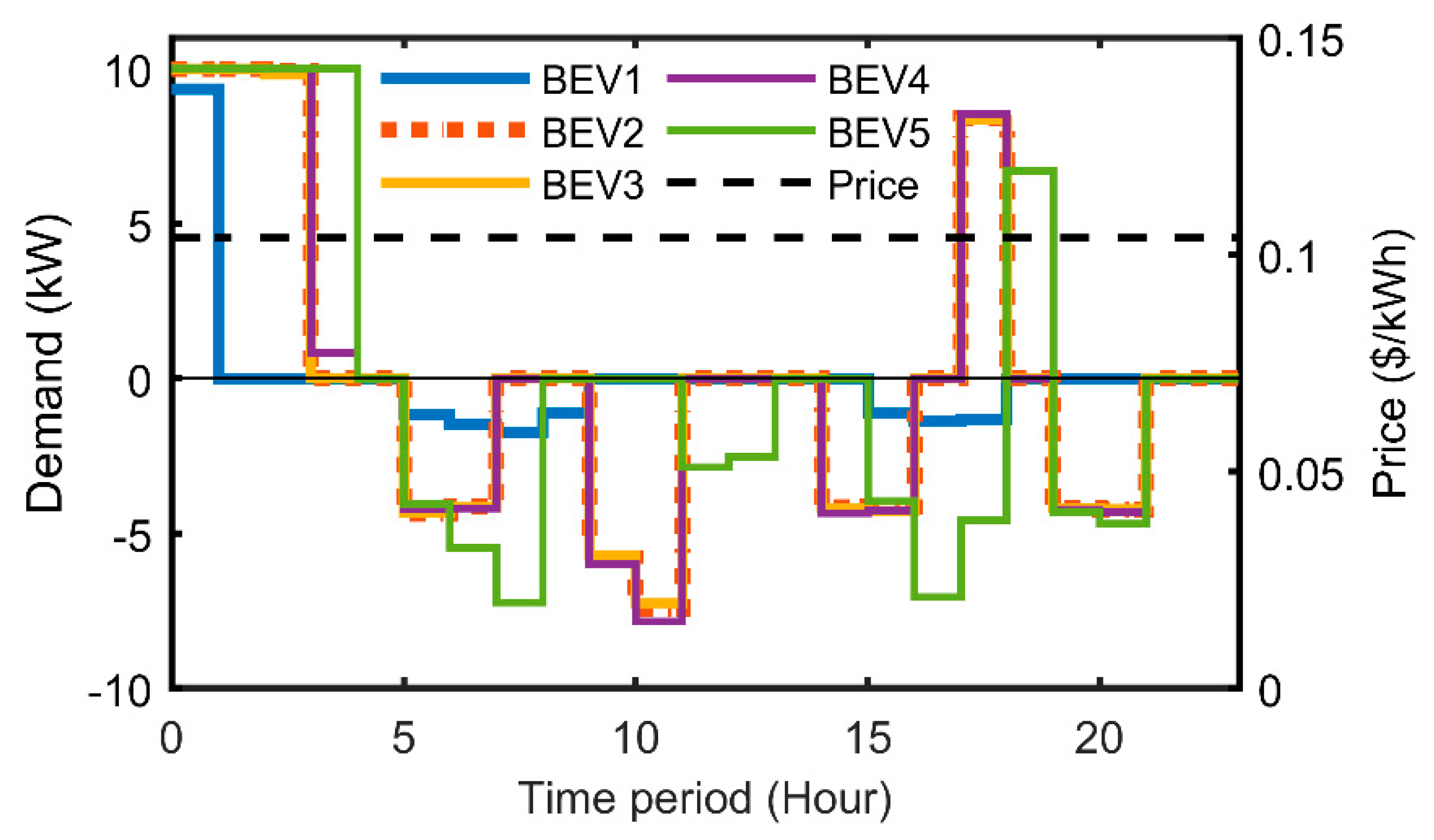Figure 5 presents a sample of the individual BEV charge/discharge schedules of five BEVs that comprise prosumer group 2 and are located in MG1.

Table 6. Aggregated BEV charge schedule and driving pattern (Case 3).

Hour	1	2	3	4	5	6	7	8	9	10	11	12
Price ($/kWh)	0.10	0.10	0.10	0.10	0.10	0.10	0.10	0.10	0.10	0.10	0.10	0.10
BEVs in MG1 (kWh)	157	110	110	81	0	−56	−70	−71	−6	−17	−23	−25
BEVs in MG2 (kWh)	177	130	126	74	0	−67	−82	−70	−5	−36	−47	−25
BEVs in MG3 (kWh)	383	270	259	143	0	−139	−167	-146	−14	−71	−93	−49
Hour	13	14	15	16	17	18	19	20	21	22	23	24
Price ($/kWh)	0.10	0.10	0.10	0.10	0.10	0.10	0.10	0.10	0.10	0.10	0.10	0.10
BEVs in MG1 (kWh)	−24	0	−13	−56	−68	−24	48	−49	−53	0	0	0
BEVs in MG2 (kWh)	−25	0	−25	−68	−68	−7	54	−63	−67	0	0	0
BEVs in MG3 (kWh)	−49	0	−51	−138	−141	−17	113	−125	−132	0	0	0

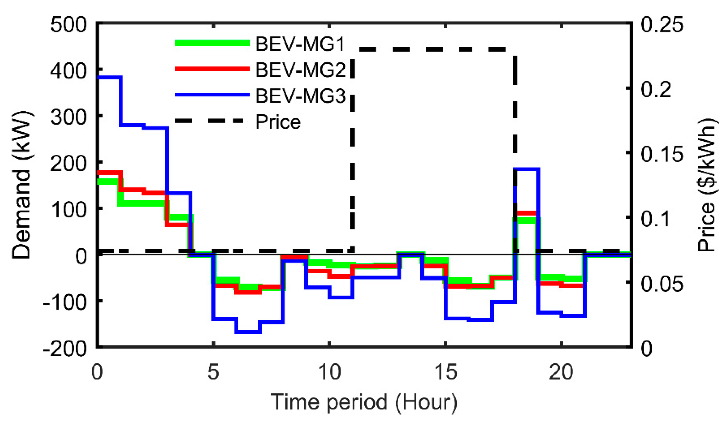
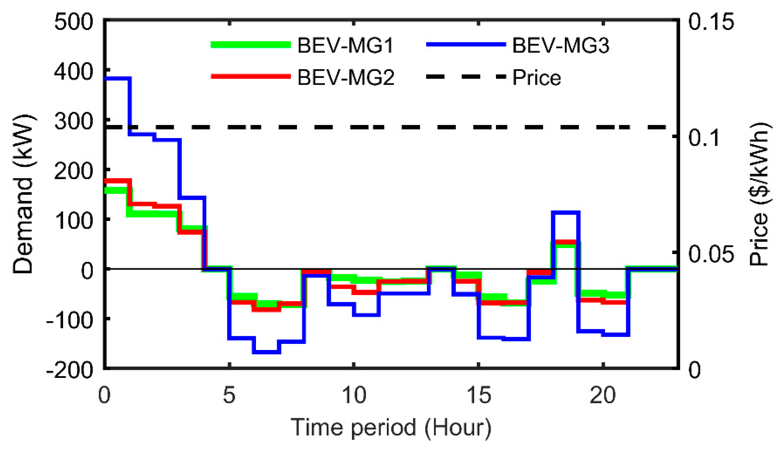
presents the numerical values of the BEV charge and usage schedule per MG. The positive values are the BEV-charging demand and the negative demand represents BEV discharging while being driven. Figure 6 presents a comparison of the BEV charge and discharge patterns in each MG. The figure illustrates the aggregated BEV drive patterns and BEV charge schedules for CGs and PCGs in MG1, MG2, and MG3. In this case, the customer charges the vehicle all night until their departure in the morning (6:00 am) and, then, another charge is conducted around (7:00 pm) to have enough energy for the commute between (8:00–9:00 pm). It is clear that, since the price is fixed throughout the day, the customer does not have any incentive to charge at a different time.

3.2. Case 4: Time-of-Use Price Signal Scenario

In this case, a Time-of-Use (TOU) price is considered for a day in summer. The TOU plans are based on the time of day and the season. By using TOU, customers can manage their energy costs. This is achieved by taking advantage of lower rates during off-peak periods and by avoiding on-peak periods when energy resources are in high demand. The TOU price that is being tested for this specific case study considers the on-peak period from 12:00 pm through 6:00 pm, Monday through Friday, for the months of June through September. The off-peak period is all other hours not covered in the on-peak period [48]. Figure 7 shows a sample of the individual BEV charge schedules and driving patterns of five BEVs that constitute prosumer group 2 and are located in MG1.

Table 7. Aggregated BEV charge schedule and driving pattern (Case 4).

Hour	1	2	3	4	5	6	7	8	9	10	11	12
Price ($/kWh)	0.07	0.07	0.07	0.07	0.07	0.07	0.07	0.07	0.07	0.07	0.07	0.23
BEVs in MG1 (kWh)	157	110	110	81	0	−56	−70	−71	−6	−17	−23	−25
BEVs in MG2 (kWh)	177	140	133	64	0	−67	−82	−70	−5	−36	−47	−25
BEVs in MG3 (kWh)	383	280	273	133	0	−139	−167	−146	−14	−71	−93	−49
Hour	13	14	15	16	17	18	19	20	21	22	23	24
Price ($/kWh)	0.23	0.23	0.23	0.23	0.23	0.23	0.07	0.07	0.07	0.07	0.07	0.07
BEVs in MG1 (kWh)	−24	0	−13	−56	−68	−50	73	−49	−53	0	0	0
BEVs in MG2 (kWh)	−25	0	−25	−68	−68	−50	89	−63	−67	0	0	0
BEVs in MG3 (kWh)	−49	0	−51	−138	−141	−102	184	−125	−132	0	0	0

presents a numerical summary of the BEV charge schedule and discharge pattern per MG. The TOU price, the aggregated BEV drive pattern, and the charge schedule within each MG are depicted in Figure 8. The optimal BEV charge schedule presented in Figure 8 is produced by using the TC+MPC. In this case, the customer charges the vehicle all night (off-peak period) until their departure in the morning. This is due to the BEV charging taking place during the off-peak period when the price is lowest. Having the price information and an incentive (lower prices) during different periods of the day allows the customers to charge their BEVs during the low-price periods. Moreover, this process is further optimized with the TC+MPC as it takes in to account the TOU information and BEV driving pattern during the day to produce a least cost schedule. By using the hybrid mechanism, the energy consumption is also minimized as the BEV is charged with the minimum energy required for the daily commute while maintaining a minimum SOC of 20%. Therefore, the customers improve their savings as they charge their vehicle in an optimal manner based on the needs for their commute.

Comparing the charge schedules with the ones obtained in Case 3, it can be seen that, having an incentive (lower price) at different times of the day, the TC+MPC increases the charging power (4–8%) between 2:00–3:00 am. The charging power is also increased (52–65%) at 7:00 pm to take advantage of the low price available after 6:00 pm.

3.3. Case 5: Dynamic Price Signal Scenario

In the final case, a dynamic price (DP) signal is considered. The price signal is based on the system DLMP (see Section 2.4). The DLMP is determined by minimizing the cost of generation considering the physical constraints of the distribution system, which exposes prosumers and consumers to the marginal cost of electricity delivery at different locations. For this case study, the DLMP accounts for marginal costs of generation and marginal costs of losses and is updated hourly.

Although the customers are receiving hourly price information, it can be difficult and time consuming for a customer to manually observe electricity prices for that specific hour and to decide when to charge their BEV. The HEMS with the embedded TC+MPC can assist the customers by automating BEV charging. The TC+MPC uses the forecasted DLMP and a forecasted BEV demand pattern to determine the optimal BEV charge schedule that minimizes the customers charging costs. The main differences with the fixed price and TOU are that the DLMP (i) is time varying (in this case hourly) and (ii) accounts for the system conditions (generation, load, and losses). Figure 9 depicts the charge schedules and driving patterns of five BEVs that are located in MG1 and are part of prosumer group 2. A detailed analysis of the numerical values of the aggregated BEV charge schedule and discharge pattern per MG is presented in

Table 8. Aggregated BEV charge schedule and driving pattern (Case 5).

Hour	1	2	3	4	5	6	7	8	9	10	11	12
Price ($/kWh)	0.09	0.08	0.08	0.08	0.08	0.09	0.09	0.09	0.09	0.09	0.10	0.10
BEVs in MG1 (kWh)	106	110	110	157	0	−56	−70	−71	−6	−17	−23	−25
BEVs in MG2 (kWh)	111	140	140	177	0	−67	−82	−70	−5	−36	−47	−25
BEVs in MG3 (kWh)	229	280	280	383	0	−139	−167	−146	−14	−71	−93	−49
Hour	13	14	15	16	17	18	19	20	21	22	23	24
Price ($/kWh)	0.10	0.10	0.10	0.11	0.11	0.11	0.10	0.10	0.10	0.10	0.09	0.09
BEVs in MG1 (kWh)	−24	0	−13	−56	−68	−50	48	−49	−53	0	0	0
BEVs in MG2 (kWh)	−25	0	−25	−68	−68	−50	34	−63	−67	0	0	0
BEVs in MG3 (kWh)	−49	0	−51	−138	−141	−102	81	−125	−132	0	0	0

.

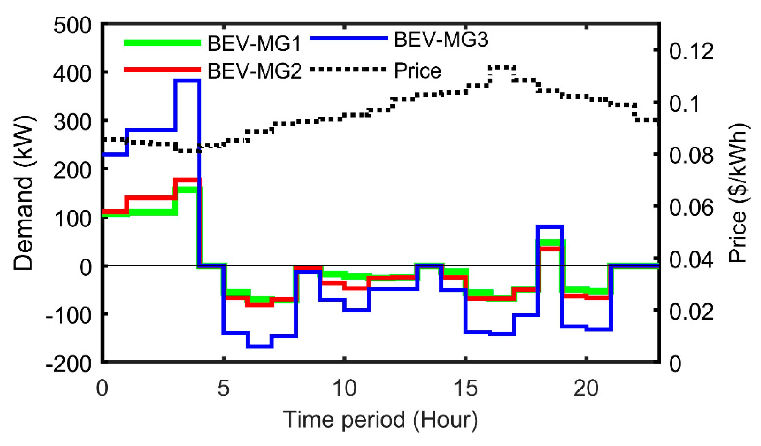
Figure 10 shows the aggregated BEVs drive pattern and the optimal charge schedule for each MG using the TC+MPC. It can be seen from Table 8 and Figure 10 how the TC+MPC optimizes the BEV charge by selecting the hours when the price is lowest. Specifically, the maximum charging occurs between 2–4 am when the price is lowest and another lower charging period occurs at 7:00 pm. When using the TC+MPC, the BEV is charged with sufficient energy for the daily commute of the customer while minimizing the costs. Comparing the results of this case with Cases 3, there is a decrease between 32–40% at 1:00 am and an increase between 94–168% at 4:00 am. These results explicitly show how the TC+MPC identifies the hours (3:00–4:00 am) with the lowest prices and maximizes the charging at those hours to avoid incurring additional costs during high-price hours. Also, incentivizing customers to charge their BEVs during low-price periods (off-peak) can reduce peak load. When compared to Case 4, there are similarities as both price signals have low-price periods. However, for the TOU, the low-price periods are fixed regardless of the distribution system conditions.

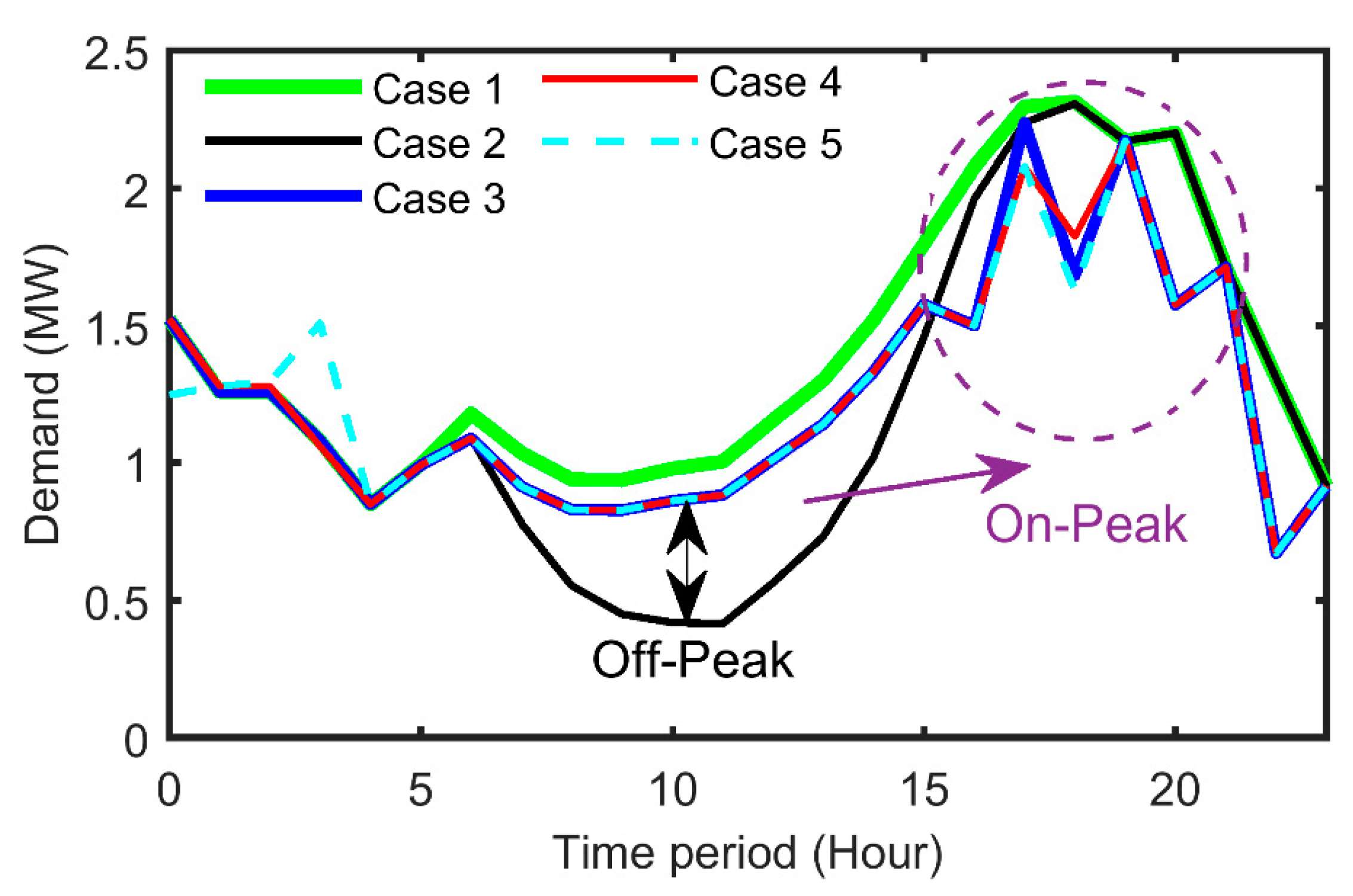
Figure 11 shows the comparison of the overall system net load for each case. Comparing the four cases with the base case (Case 1), it can be seen that the overall system net load is lower for all the cases, which is due to the solar PV power output. It can also be seen from Figure 11 that having BESS available allows the prosumers to shift the surplus power production of solar PV (from 7:00 am to 3:00 pm) to peak load periods (between 6:00 and 10:00 pm). Shifting surplus power from off-peak periods can reduce peak load from 21–30% (489–685kW). Moreover, storing the solar PV surplus power can reduce load ramp rates from 39–58% (136–196kW/h). It can also be seen in Figure 11 that, due to the BESS discharge during the peak period, the demand curve becomes more volatile and steep load ramps (from 347–542kW/h) are created. This an undesirable effect, and it becomes an important aspect to consider when setting the BESS discharge constraints in order to minimize negative impacts due to the BESS discharge.

As it was explained in Section 2.1, a power-flow simulation is conducted to calculate system power losses and bus voltage profiles. The power-flow results are obtained using MATPOWER [59]. In MATPOWER, when BEVs and BESS are charging, these are treated as load. For every hour, an energy balance is conducted at each bus, i.e., solar PV power is subtracted from the load (household load+BEV and BESS charge). If the net load is negative (i.e., solar PV power generation is greater than the load), then the bus becomes a PV bus. On the other hand, if the net load is positive, the bus remains as a PQ bus. Once the values are assigned for the time period (1 h), the power flow is executed. This process is repeated for the simulation horizon of 24 h.

Table 9. Comparison of total system power losses.

	Power Losses (kW)	Reduction (%)
Case 1 (Without PV or BESS)	1788	0%
Case 2 (Without BESS)	1582	11.5%
Case 3 (Fixed Price)	1672	6.5%
Case 4 (TOU Price)	1676	6.3%
Case 5 (Dynamic Price)	1667	6.8%

shows a comparison of the total system losses for each case. Comparing the overall system losses of Cases 2–5 with the base case (Case 1), it can be seen that all the cases reduce power losses and that the highest reduction in losses (11.5%) is achieved in Case 2. Case 2 assumes customers have BEVs and rooftop solar PV installations, and any surplus PV power is injected back to the utility grid. Cases 3–5 achieve an overall system power loss reduction of 6.5%, 6.3%, and 6.8%, respectively, compared to the base case (Case 1). It is worth noting that the reduction in power losses that is achieved in the case studies can be dependent on the location of the DERs in the distribution network. As previous research has shown, the location of DERs can reduce power losses and, in some cases, increase them [42]. The difference in power loss reduction between Case 2 and Cases 3–5 can be attributed to power losses in storing surplus power in the BESS and to the residual energy that remains stored in the BESS. Although there is a higher power loss reduction in Case 2 compared to Cases 3–5, there are other benefits achieved in Cases 3–5. These benefits are (i) reduction in peak load, (ii) minimization of charging costs for BEV owners, and (iii) participation in a retail electricity market and maximization of savings by prosumers by using the power stored in the BESS during high-price periods. Benefit number (iii) gives the customers flexibility to use the energy for their own use or to sell to other customers when high prices are available.

Voltage profiles are also analyzed to observe the effects produced by the BEV-charging and BESS-discharge schedules for each case.

Table 10. Summary of bus voltage improvements.

		Hours Under Voltage (<0.95 p.u.)	Hour Difference			Hours Under Voltage (<0.95 p.u.)	Hour Difference
Bus	Case			Bus	Case
9	1	4	0	17	1	11	0
	2	4	0		2	7	−4
	3	2	−2		3	6	−5
	4	1	−3		4	6	−5
	5	1	−3		5	6	−5
10	1	5	0	18	1	11	0
	2	4	−1		2	7	−4
	3	2	−3		3	6	−5
	4	2	−3		4	6	−5
	5	2	−3		5	6	−5
11	1	6	0	28	1	5	0
	2	4	−2		2	4	−1
	3	2	−4		3	2	−3
	4	2	−4		4	2	−3
	5	2	−4		5	2	−3
12	1	7	0	29	1	8	0
	2	5	−2		2	5	−3
	3	3	−4		3	5	−3
	4	3	−4		4	5	−3
	5	3	−4		5	5	−3
13	1	8	0	30	1	10	0
	2	5	−3		2	6	−4
	3	4	−4		3	5	−5
	4	6	−2		4	5	−5
	5	6	−2		5	5	−5
14	1	9	0	31	1	12	0
	2	6	−3		2	7	−5
	3	6	−3		3	7	−5
	4	6	−3		4	7	−5
	5	6	−3		5	7	−5
15	1	9	0	32	1	13	0
	2	6	−3		2	8	−5
	3	6	−3		3	9	−4
	4	6	−3		4	9	−4
	5	6	−3		5	8	−5
16	1	11	0	33	1	13	0
	2	7	−4		2	8	−5
	3	6	−5		3	9	−4
	4	6	−5		4	9	−4
	5	6	−5		5	9	−4

presents a comparative summary of bus voltage violations (undervoltages) that were recorded when running the simulations as well as improvements to the bus voltage profiles. It should be mentioned that no overvoltages were observed in any of the buses of the test system. The bus voltages that are not shown in Table 10 did not present violations (over/under voltages). The comparative analysis summarized in Table 10 is done between the base case (Case 1) and Cases 2–5. The values shown in the undervoltage column indicate the number of hours an undervoltage has been recorded in the corresponding case. The values presented in the difference column indicate the difference in number of hour(s) that the corresponding case recorded an undervoltage compared to the base case (Case 1). A negative sign (−) indicates a reduction in hour(s), a positive sign (+) indicates an increase in hour(s), and a zero (0) indicates no difference.

By further analyzing the results presented in Table 10, it can be stated that having rooftop solar PV installations (Case 2) can improve bus voltage profiles from 20% and up to 42% compared to the base case (Case 1). However, having a hybrid PV-BESS system (Cases 3–5) can improve voltage profiles between 25% and 75% compared to the base case. In all but one bus (Bus 33), the cases where BESS is present render a higher voltage profile improvement. Thus, having controllable demand-side DER can protect the system from overvoltages that can be incurred in the uncontrolled case (Case 2) while also providing the benefits that have been previously discussed.

Finally, a cost/savings analysis is carried out to compare the total daily costs and savings for the PCGs and CGs located in each MG. The daily costs and savings data are presented in

Table 11. Total Daily Costs ($) and Savings ($) Comparison per Microgrid.

		Case 1		Case 2		Case 3
		Total Costs	Total Savings	Total Costs	Total Savings	Total Costs	Total Savings
	PCG1	54.66	0.00	40.96	13.70	31.36	23.30
MG1	PCG2	70.65	0.00	51.90	18.75	37.60	33.05
	CG1	52.99	0.00	52.99	0.00	52.99	0.00
	PCG3	51.79	0.00	36.17	15.62	27.32	24.47
MG2	CG2	43.84	0.00	43.84	0.00	43.84	0.00
	PCG4	55.85	0.00	39.41	16.44	29.93	25.92
	PCG5	43.54	0.00	30.91	12.64	23.88	19.66
	CG3	108.42	0.00	108.42	0.00	108.42	0.00
	CG4	165.86	0.00	165.86	0.00	165.86	0.00
MG3	PCG6	89.73	0.00	62.33	27.40	46.09	43.64
	PCG7	92.15	0.00	60.90	31.25	44.63	47.52
	CG5	72.44	0.00	72.44	0.00	72.44	0.00
	PCG8	91.00	0.00	64.67	26.33	50.99	40.01
		Case 4		Case 5
		Total Costs	Total Savings	Total Costs	Total Savings
	PCG1	25.50	31.90	39.79	29.63
MG1	PCG2	33.15	45.76	45.73	41.98
	CG1	53.29	0.00	65.07	0.00
	PCG3	21.52	36.59	34.44	29.19
MG2	CG2	42.65	0.00	55.63	0.00
	PCG4	23.72	38.19	35.04	32.01
	PCG5	18.54	24.92	27.15	24.66
	CG3	118.57	0.00	134.84	0.00
	CG4	202.87	0.00	209.43	0.00
MG3	PCG6	37.72	63.07	71.20	56.12
	PCG7	36.74	71.29	62.49	62.32
	CG5	25.50	31.90	39.79	29.63
	PCG8	33.15	45.76	45.73	41.98

and

Table 12. Net costs ($) comparison per microgrid.

		Case 1		Case 2		Case 3
		Net Costs ($)	Inc./Red. (%)	Net Costs ($)	Inc./Red. (%)	Net Costs ($)	Inc./Red. (%)
	PCG1	54.66	0.00	27.26	−50.13	8.06	−85.25
MG1	PCG2	70.65	0.00	33.15	−53.07	4.55	−93.57
	CG1	52.99	0.00	52.99	0.00	52.99	0.00
	PCG3	51.79	0.00	20.54	−60.33	2.85	−94.50
MG2	CG2	43.84	0.00	43.84	0.00	43.84	0.00
	PCG4	55.85	0.00	22.97	−58.87	4.01	−92.81
	PCG5	43.54	0.00	18.27	−58.05	4.22	−90.31
	CG3	108.42	0.00	108.42	0.00	108.42	0.00
	CG4	165.86	0.00	165.86	0.00	165.86	0.00
MG3	PCG6	89.73	0.00	34.93	−61.07	2.44	−97.28
	PCG7	92.15	0.00	29.66	−67.82	−2.90	−103.14
	CG5	72.44	0.00	72.44	0.00	72.44	0.00
	PCG8	91.00	0.00	38.34	−57.87	10.97	−87.94
		Case 4		Case 5
		Net Costs ($)	Inc./Red. (%)	Net Costs ($)	Inc./Red. (%)
	PCG1	−6.40	−111.7	10.17	−81.40
MG1	PCG2	−12.61	−117.8	3.75	−94.69
	CG1	53.29	0.57	65.07	22.79
	PCG3	−15.06	−129.1	5.26	−89.85
MG2	CG2	42.65	−2.73	55.63	26.89
	PCG4	−14.47	−125.9	3.03	−94.58
	PCG5	−6.38	−114.6	2.49	−94.28
	CG3	118.57	9.37	134.84	24.37
	CG4	202.87	22.31	209.43	26.27
MG3	PCG6	−25.35	−128.2	15.08	−83.20
	PCG7	−34.55	−137.5	0.17	−99.82
	CG5	72.33	−0.14	103.88	43.41
	PCG8	−14.18	−115.6	40.30	−55.71

. In Table 11, the Costs ($) refer to the amount paid for the daily energy consumption and Savings ($) refer to energy cost reduction associated to the use of rooftop solar PV and BESS.

Comparing the results of the five cases (see Table 11), we can observe that the highest overall savings are achieved by PCGs in Cases 4 (TOU) and 5 (DP). Also, Cases 3–5 produced greater savings than Cases 1 and 2. Specifically, the savings differences were between 52–76% (Case 3), 128–144% (Case 4), and 95–123% (Case 5). When comparing the costs of Cases 2–5 to those of Case 1 (base case), they all achieve a cost reduction. The total cost reductions compared to Case 1 for Case 2 is 29%, for Case 3 is 45%, for Case 4 is 57%, and for Case 5 is 37%.

The results comparison demonstrates that, by having the BESS, the reduction in total costs for Cases 3–5 is improved. This is more noticeable in Case 5 as the demand during high-price periods is fulfilled by the energy stored in the BESS. With the reduction of the peak demand between 6:00 pm and 9:00 pm (see Figure 11), there is an associated reduction in electricity price, which in turn has a significant impact on the total costs of the CGs and PCGs. We can clearly observe that, by shifting the surplus PV generation with BESS (controlled by TC) to peak load hours, PCGs can reduce their total energy costs.

Table 12 presents the comparison of net costs and the difference between each case and the base case. In Table 12, Net Costs are the costs minus savings (Costs − Savings) and the percentage column indicates an increase (Inc.) if it is positive and a reduction (Red.) if negative.

Further analysis of the net costs results (see Table 12) shows that Case 4 achieves the highest net cost reduction percentages for both CGs and PCGs followed by Case 5, which produces a higher net cost reduction for PCGs. Also, CGs achieve more net cost reduction under the fixed and TOU pricing schemes (Cases 3 and 4) compared to a DP scheme (Case 5). These results are reasonable as CGs do not possess alternative sources of generation to fulfill their own demand and can only participate by deferring or shifting loads to low-price periods.

Therefore, it can be inferred that a DP scheme is better suited for PCGs that are able to respond to price signals via BESS or other controllable distributed generation sources. It should be noted that, for simulation purposes, in Case 2–5, the price signal is considered the same for buying and selling power (net metering). In different electricity markets, utilities and DSOs have lower paying costs for selling power to the grid. Consequently, the total savings for Cases 2–4 could be lower under these pricing schemes when compared to Case 5, thus adding more value to TC+MPC and BESS for customers under those pricing schemes.

It should be noted that the test results are only representatives and are obtained under simulated conditions for the considered test system. More case studies could be further conducted for longer time horizons (e.g., weeks and months) with different scenarios, test systems, and MG locations in order to be able to conclude that the benefits mentioned in the case studies will be achieved with high certainty.

The TC+MPC formulation presented in this paper has been implemented in MATLAB R2017a and solved with YALMIP and GUROBI (Gurobi Optimization, LLC., Beaverton, OR, USA). MATLAB (The MathWorks Inc., Natick, MA, USA) is used as the programming environment, while YALMIP structures the optimization problem into matrices with the objective function, the optimization variables, and the equality and inequality constraints [60]. GUROBI is used as an external solver to find the optimal solution of the problem [61]. All simulations were conducted using a personal computer with 2.8 GHz CPU, 4 GB RAM.

4. Conclusions

This paper presented a new hybrid TC+MPC control mechanism for residential prosumer-centric networked MGs. The proposed hybrid TC+MPC combines the control capabilities and features of the MPC and the TC, creating a robust control mechanism that is driven by transactive incentive signals, and thus, also providing the MGEMS capability to deal with the stochastic nature of BEV driving by using a MCS to generate the BEV driving patterns. The proposed TC+MPC was able to effectively generate the BEV-charge and BESS-discharge schedules for the CGs/PCGs located in each MG. Test results demonstrated the potential of using pricing mechanisms for demand-side management of DERs. The results can be summarized as follows: (i) reduction in peak load (between 21–30%) by shifting surplus PV power from off-peak hours using BESS; (ii) reduction in load ramp rates between 39–58%; (iii) reduction in power losses between 6.3–6.8%; (iv) bus voltage improvements between 25–75% for busses that present undervoltages; and (v) total cost reductions between 29–57% and savings between 52–144%. Therefore, the main objectives of the MGEMS are met by allowing CGs/PCGs to minimize their costs as well as to maximize their savings. It can also be inferred from the results that the incentives provided by the pricing mechanisms can encourage customers to not only reduce peak demand but also to install more demand-side energy resources (e.g., but not limited to BESS and rooftop solar). Moreover, the DSO or utility operators can benefit from controlled customer participation by reducing their system power losses, by improving bus voltage profiles, and by reducing overloading system components. An important finding of the case studies is that the BESS-discharging operation can create steep load ramp rates when discharging during peak periods. This aspect should be considered high priority when defining the discharge constraints to avoid incurring negative impacts on the grid. For the case studies presented in this paper, we assumed full BESS discharging (SOC = 0%). It should be noted that this discharging operation could impact the expected life of the BESS. Future work would be interesting to study the depth of discharge impacts on the BESS life cycle and, then, to expand it to larger time frames (e.g., months and years) to analyze the effects of continuous BEV and BESS charge/discharge cycles. From an economic perspective, different TOU tariffs could also be tested to further verify the capabilities of the TC and costs associated to DER purchase and installation could be included to better reflect the net costs/savings. Finally, from a utility perspective, a study of reliability and resiliency impacts on distribution networks due to the use of TCs and DERs can also be considered in future work.

References

1. GridWise Architecture Council. GridWise Transactive Energy Framework; Technical Report; GridWise Architecture Council: Richland, WA, USA, 2017. [Google Scholar]
2. Cazalet, E.; De Martini, P.; Price, J.; Woychik, E.; Caldwell, J. Transactive energy models. In NIST Transactive Energy Challenge: Business and Regulatory Models; White Paper; National Institute of Standards and Technology: Gaithersburg, MD, USA, 2016. [Google Scholar]
3. GridWise Architecture Council. Transactive Energy Systems Research, Development and Deployment Roadmap; White Paper; GridWise Architecture Council: Richland, WA, USA, 2018. [Google Scholar]
4. U.S. Energy Information Administration. Electricity Data Browser Net Generation by Energy Source: 2001–2018. 2019. Available online: https://www.eia.gov/electricity/annual/html/epa_03_01_a.html (accessed on 13 April 2019).
5. U.S. Energy Information Administration. Annual Energy Outlook 2019 with Projections to 2050. 2019. Available online: https://www.eia.gov/aeo (accessed on 15 January 2019).
6. International Energy Agency-IEA. Global EV Outlook 2018; Technical Report; International Energy Agency-IEA: Paris, France, 2018. [Google Scholar]
7. Parhizi, S.; Lotfi, H.; Khodaei, A.; Bahramirad, S. State of the art in research on microgrids: A review. IEEE Access 2015, 3, 890–925. [Google Scholar] [CrossRef]
8. Alam, M.N.; Chakrabarti, S.; Ghosh, A. Networked microgrids: State-of-the-art and future perspectives. IEEE Trans. Ind. Inform. 2019, 15, 1238–1250. [Google Scholar] [CrossRef]
9. Li, Z.; Shahidehpour, M.; Aminifar, F.; Alabdulwahab, A.; Al-Turki, Y. Networked microgrids for enhancing the power system resilience. Proc. IEEE 2017, 105, 1289–1310. [Google Scholar] [CrossRef]
10. Zamora, R.; Srivastava, A.K. Multi-layer architecture for voltage and frequency control in networked microgrids. IEEE Trans. Smart Grid 2018, 9, 2076–2085. [Google Scholar] [CrossRef]
11. Schneider, K.P.; Radhakrishnan, N.; Tang, Y.; Tuffner, F.K.; Liu, C.C.; Xie, J.; Ton, D. Improving primary frequency response to support networked microgrid operations. IEEE Trans. Power Syst. 2019, 34, 659–667. [Google Scholar] [CrossRef]
12. Sandgani, M.R.; Sirouspour, S. Priority-based microgrid energy management in a network environment. IEEE Trans. Sustain. Energy 2018, 9, 980–990. [Google Scholar] [CrossRef]
13. Shi, W.; Xie, X.; Chu, C.C.; Gadh, R. Distributed optimal energy management in microgrids. IEEE Trans. Smart Grid 2015, 6, 1137–1146. [Google Scholar] [CrossRef]
14. Jadhav, A.M.; Patne, N.R. Priority-based energy scheduling in a smart distributed network with multiple microgrids. IEEE Trans. Ind. Inform. 2017, 13, 3134–3143. [Google Scholar] [CrossRef]
15. Gregoratti, D.; Matamoros, J. Distributed energy trading: The multiple-microgrid case. IEEE Trans. Ind. Electron. 2015, 62, 2551–2559. [Google Scholar] [CrossRef]
16. Ramli, M.A.M.; Bouchekara, H.R.E.H.; Alghamdi, A.S. Efficient energy management in a microgrid with intermittent renewable energy and storage sources. Sustainability 2019, 11, 3839. [Google Scholar] [CrossRef]
17. Yue, J.; Hu, Z.; Anvari-Moghaddam, A.; Guerrero, J.M. A multi-market-driven approach to energy scheduling of smart microgrids in distribution networks. Sustainability 2019, 11, 301. [Google Scholar] [CrossRef]
18. Aslam, S.; Javaid, N.; Khan, F.A.; Alamri, A.; Almogren, A.; Abdul, W. Towards efficient energy management and power trading in a residential area via integrating a grid-connected microgrid. Sustainability 2018, 10, 1245. [Google Scholar] [CrossRef]
19. Liu, Z.; Wu, Q.; Huang, S.; Zhao, H. Transactive energy: A review of state of the art and implementation. In Proceedings of the 2017 IEEE Manchester PowerTech, Manchester, UK, 18–22 June 2017; pp. 1–6. [Google Scholar]
20. Pacific Northwest Smartgrid Demonstration Project. Technology Performance Report Highlights; Technical Report; Pacific Northwest National Laboratory: Richland, WA, USA, 2015.
21. Li, J.; Zhang, C.; Xu, Z.; Wang, J.; Zhao, J.; Zhang, Y.J.A. Distributed transactive energy trading framework in distribution networks. IEEE Trans. Power Syst. 2018, 33, 7215–7227. [Google Scholar] [CrossRef]
22. Nunna, H.S.V.S.K.; Srinivasan, D. Multiagent-based transactive energy framework for distribution systems with smart microgrids. IEEE Trans. Ind. Inform. 2017, 13, 2241–2250. [Google Scholar] [CrossRef]
23. Amanbek, Y.; Tabarak, Y.; Nunna, H.S.V.S.K.; Doolla, S. Decentralized transactive energy management system for distribution systems with prosumer microgrids. In Proceedings of the 19th International Carpathian Control Conference, Szilvasvarad, Hungary, 28–31 May 2018; pp. 553–558. [Google Scholar]
24. Renani, Y.K.; Ehsan, M.; Shahidehpour, M. Optimal transactive market operations with distribution system operators. IEEE Trans. Smart Grid 2018, 9, 6692–6701. [Google Scholar] [CrossRef]
25. Liu, Z.; Wu, Q.; Ma, K.; Shahidehpour, M.; Xue, Y.; Huang, S. Two-stage optimal scheduling of electric vehicle charging based on transactive control. IEEE Trans. Smart Grid 2019, 10, 2948–2958. [Google Scholar] [CrossRef]
26. Liu, Z.; Wu, Q.; Shahidehpour, M.; Li, C.; Huang, S.; Wei, W. Transactive real-time electric vehicle charging management for commercial buildings with pv on-site generation. IEEE Trans. Smart Grid 2018, 10, 4939–4950. [Google Scholar] [CrossRef]
27. Hu, J.; Yang, G.; Bindner, H.W. Network constrained transactive control for electric vehicles integration. In Proceedings of the 2015 IEEE Power & Energy Society General Meeting, Denver, CO, USA, 26–30 July 2015; pp. 1–5. [Google Scholar]
28. Shigenobu, R.; Kinjo, M.; Mandal, P.; Howlader, A.; Senjyu, T. Optimal operation method for distribution systems considering distributed generators imparted with reactive power incentive. Appl. Sci. 2018, 8, 1411. [Google Scholar] [CrossRef]
29. Wang, H.; Huang, J. Incentivizing energy trading for interconnected microgrids. IEEE Trans. Smart Grid 2018, 9, 2647–2657. [Google Scholar] [CrossRef]
30. Liu, W.; Zhan, J.; Chung, C.Y. A novel transactive energy control mechanism for collaborative networked microgrids. IEEE Trans. Power Syst. 2019, 34, 2048–2060. [Google Scholar] [CrossRef]
31. Khodayar, M.E.; Manshadi, S.D.; Vafamehr, A. The short-term operation of microgrids in a transactive energy architecture. Electr. J. 2016, 29, 41–48. [Google Scholar] [CrossRef]
32. Jingpeng, Y.; Zhijian, H.; Chendan, L.; Vasquez, J.C.; Guerrero, J.M. Economic power schedule and transactive energy through an intelligent centralized energy management system for a dc residential distribution system. Energies 2017, 10, 916. [Google Scholar]
33. Prinslooa, G.; Mammolib, A.; Dobsona, R. Customer domain supply and load coordination: A case for smart villages and transactive control in rural off-grid microgrids. Energy 2017, 135, 430–441. [Google Scholar] [CrossRef]
34. Canizes, B.; Soares, J.; Costa, A.; Pinto, T.; Lezama, F.; Novais, P.; Vale, Z. Electric vehicles’ user charging behavior simulator for a smart city. Energies 2019, 12, 1470. [Google Scholar] [CrossRef]
35. Dubey, A.; Santoso, S. Electric vehicle charging on residential distribution systems: Impacts and mitigations. IEEE Access 2015, 3, 1871–1893. [Google Scholar] [CrossRef]
36. Suyono, H.; Rahman, M.T.; Mokhlis, H.; Othman, M.; Azil Illias, H.; Mohamad, H. Optimal scheduling of plug-in electric vehicle charging including time-of-use tariff to minimize cost and system stress. Energies 2019, 12, 1500. [Google Scholar] [CrossRef]
37. Chekired, D.A.; Khoukhi, L.; Mouftah, H.T. Decentralized cloud-SDN architecture in smart grid: A dynamic pricing model. IEEE Trans. Ind. Inform. 2018, 14, 1220–1231. [Google Scholar] [CrossRef]
38. Pasetti, M.; Rinaldi, S.; Flammini, A.; Longo, M.; Foiadelli, F. Assessment of electric vehicle charging costs in presence of distributed photovoltaic generation and variable electricity tariffs. Energies 2019, 12, 499. [Google Scholar] [CrossRef]
39. Liu, S.; Etemadi, A.H. A dynamic stochastic optimization for recharging plug-in electric vehicles. IEEE Trans. Smart Grid 2018, 9, 4154–4161. [Google Scholar] [CrossRef]
40. Pantos, M. Exploitation of electric-drive vehicles in electricity markets. IEEE Trans. Power Syst. 2012, 27, 682–694. [Google Scholar] [CrossRef]
41. Camacho, E.F.; Bordons, C. Model Predictive Control, 2nd ed.; Springer: London, UK, 2007; pp. 1–30. [Google Scholar]
42. Galvan, E.; Mandal, P.; Haque, A.U.; Tseng, B. Optimal placement of intermittent renewable energy resources and energy storage system in smart power distribution networks. Electr. Power Compon. Syst. 2017, 45, 1543–1553. [Google Scholar] [CrossRef]
43. Galvan, E.; Mandal, P.; Chakraborty, S.; Saber, A.Y. Efficient transactive control for energy storage management system in prosumer-centric networked microgrids. In Proceedings of the 2018 North American Power Symposium (NAPS), Fargo, ND, USA, 9–11 September 2019; pp. 1–6. [Google Scholar]
44. International Energy Agency (IEA). Global EV Outlook: Towards Cross-Modal Electrification; Technical Report; IEA: Paris, France, 2018. [Google Scholar]
45. United States Census Bureau. Comparative Housing Characteristics. Available online: https://factfinder.census.gov/faces/tableservices/jsf/pages/productview.xhtml?pid=ACS_17_5YR_CP04&prodType=table (accessed on 15 January 2019).
46. Baran, M.E.; Wu, F.F. Network reconfiguration in distribution systems for loss reduction and load balancing. IEEE Trans. Power Deliv. 1989, 4, 1401–1407. [Google Scholar] [CrossRef]
47. El Paso Electric Company. Residential Service Rate 2018. Available online: https://www.epelectric.com/files/html/Rates_and_Regulatory/Docket_46831_Stamped_Tariffs/03_-_Rate_01_Residential_Service_Rate.pdf (accessed on 15 January 2019).
48. El Paso Electric Company. Electric Vehicle Charging Rate 2018. Available online: https://www.epelectric.com/files/html/Rates_and_Regulatory/Docket_46831_Stamped_Tariffs/36_-_Rate_EVC_Electric_Vehicle_Charging_Rate.pdf (accessed on 15 January 2019).
49. PJM. Price Data. Available online: http://www.pjm.com/markets-and-operations/energy.aspx (accessed on 15 January 2019).
50. U.S. Department of Energy, Office of Energy Efficiency & Renewable Energy (EERE) Open Data Catalog. Residential Load at TMY3. Available online: https://openei.org/datasets/files/961/pub/ (accessed on 15 January 2019).
51. InsideEVs.com. Available online: https://insideevs.com/reviews/344001/compare-evs/ (accessed on 30 August 2019).
52. Edison Electric Institute (EEI). Electric Vehicle Sales: Facts & Figures. Available online: https://www.eei.org/issuesandpolicy/electrictransportation/Documents/FINAL_EV_Sales_Update_April2019.pdf (accessed on 30 August 2019).
53. Tesla Motors. Tesla Charging. 2019. Available online: https://www.tesla.com/models-charging#/basics (accessed on 30 May 2019).
54. Quiros-Tortos, J.; Ochoa, L.F.; Butler, T. How electric vehicles and the grid work together: Lessons learned from one of the largest electric vehicle trials in the world. IEEE Power Energy Mag. 2018, 16, 64–76. [Google Scholar] [CrossRef]
55. Idaho National Laboratory, U.S. Department of Energy Office of Energy Efficiency and Renewable Energy. Plug-in Electric Vehicle and Infrastructure Analysis; Technical Report; Idaho National Laboratory, U.S. Department of Energy Office of Energy Efficiency and Renewable Energy: Washington, DC, USA, 2015.
56. Tesla Motors. Tesla Powerwall. 2019. Available online: https://www.tesla.com/powerwall (accessed on 15 January 2019).
57. Trabish, H.K. Utility Dive. What Will Electricity Pricing Look Like in 2040? August 2019. Available online: https://www.utilitydive.com/news/what-will-electricity-pricing-look-like-in-2040/558708/ (accessed on 13 September 2019).
58. California Public Utilities Commission (CPUC). Residential Rate Reform/R.12-06-013. Available online: https://www.cpuc.ca.gov/General.aspx?id=12154 (accessed on 13 September 2019).
59. Zimmerman, R.D.; Murillo-Sánchez, C.E.; Thomas, R.J. MATPOWER: Steady-state operations, planning and analysis tools for power systems research and education. IEEE Trans. Power Syst. 2011, 26, 12–19. [Google Scholar] [CrossRef]
60. YALMIP. Available online: https://yalmip.github.io/ (accessed on 15 January 2019).
61. GUROBI. Available online: https://www.gurobi.com/ (accessed on 15 January 2019).
Figure 1. Sample of a residential Microgrid (MG).
Sustainability 11 05436 g001
Figure 2. Flowchart of the proposed optimization and control procedure.
Sustainability 11 05436 g002
Figure 3. Networked microgrids in an IEEE 33-bus distribution network.
Sustainability 11 05436 g003
Figure 4. Residential solar photovoltaic (PV) power output profile on a sunny summer day.
Sustainability 11 05436 g004
Figure 5. Optimal charge schedule and driving pattern of BEVs located in PCG2-MG1 (Case 3).
Sustainability 11 05436 g005
Figure 6. Aggregated BEV charge schedule and driving pattern of the three MGs (Case 3).
Sustainability 11 05436 g006
Figure 7. Optimal charge schedule and driving pattern of BEVs located in PCG2-MG1 (Case 4).
Sustainability 11 05436 g007
Figure 8. Aggregated BEV charge schedule and driving pattern of the three MGs (Case 4).
Sustainability 11 05436 g008
Figure 9. Optimal charge schedule and driving pattern of BEVs located in PCG2-MG1 (Case 5).
Sustainability 11 05436 g009
Figure 10. Aggregated BEV charge schedule and driving pattern of the three MGs (Case 5).
Sustainability 11 05436 g010
Figure 11. Overall system net load comparison for each case.
Sustainability 11 05436 g011