Analysis of Prediction Accuracy under the Selection of Optimum Time Granularity in Different Metro Stations

Abstract
:1. Introduction
2. Study Area and Data
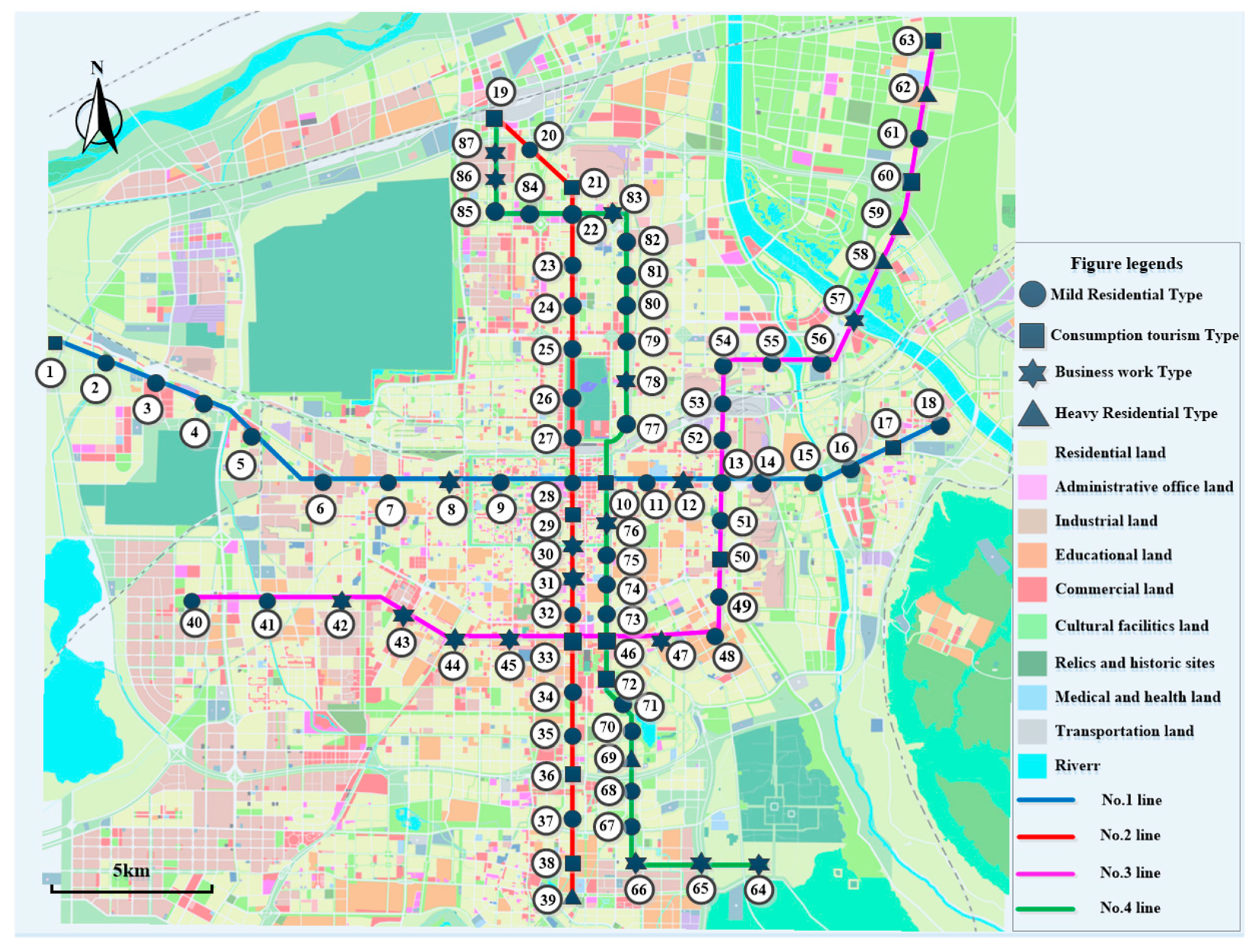
2.1. Study Area
2.2. Data Acquisition and Preliminary Analysis
3. Methodology
3.1. Cluster Analysis of Station
3.1.1. K-means Clustering Method
3.1.2. Selection of Clustering Factors
3.1.3. Case Analysis of Station Clustering
3.2. Time Granularity Study
3.2.1. Selection Range of Time Granularity
3.2.2. Time Granularity Selection
3.2.3. Selection Range of the Optimum Time Period
3.3. EMD-SVR Prediction Method
3.3.1. Process of Data De-noising
3.3.2. SVR Model Prediction
3.4. Prediction Result Analysis and Model Performance Comparision
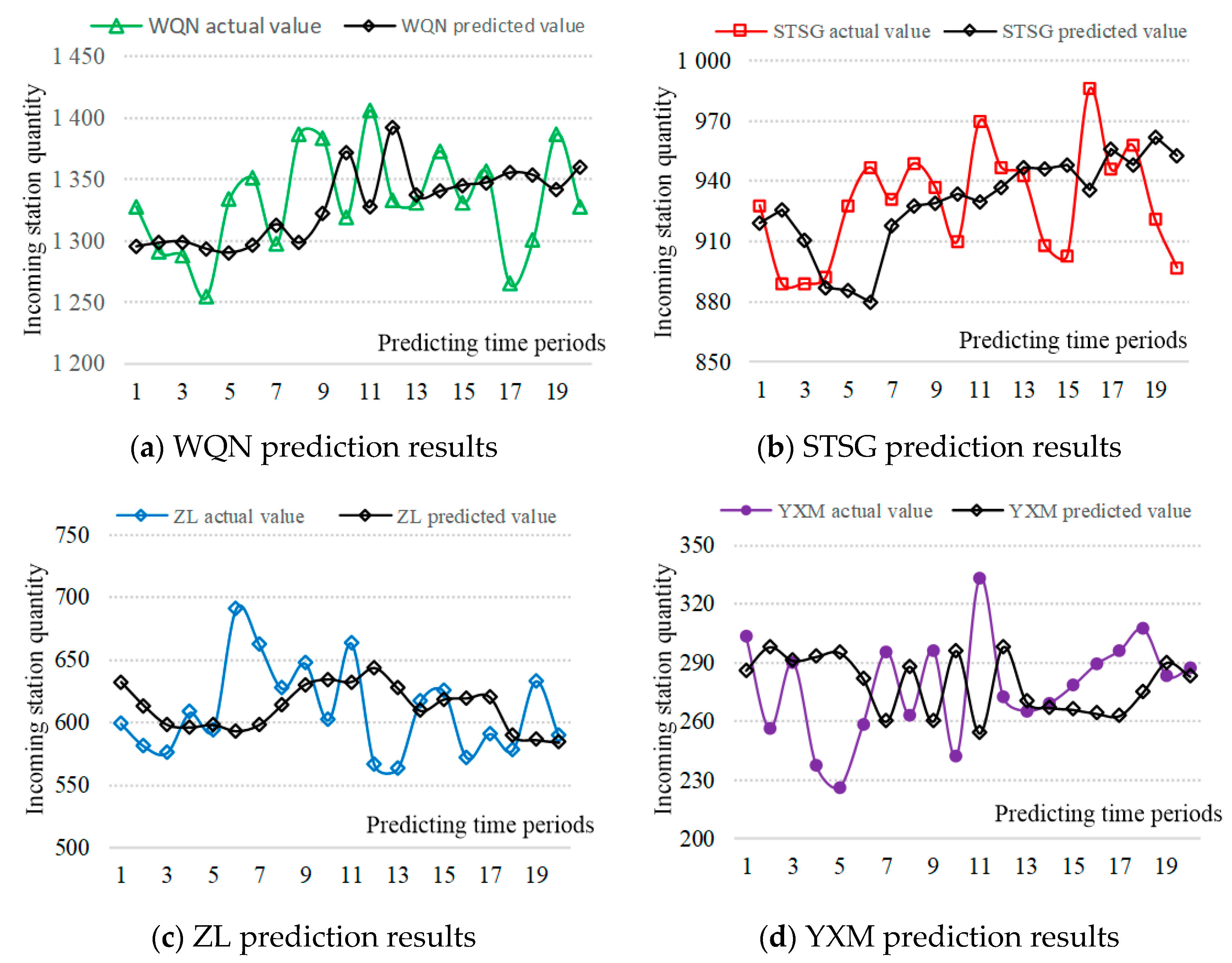
3.4.1. Prediction Result Analysis
3.4.2. BPNN Prediction Model Introduction
3.4.3. Comparative Analysis of Predicting Results (EMD-SVR) and Other Methods
4. Results and Analysis
5. Conclusions
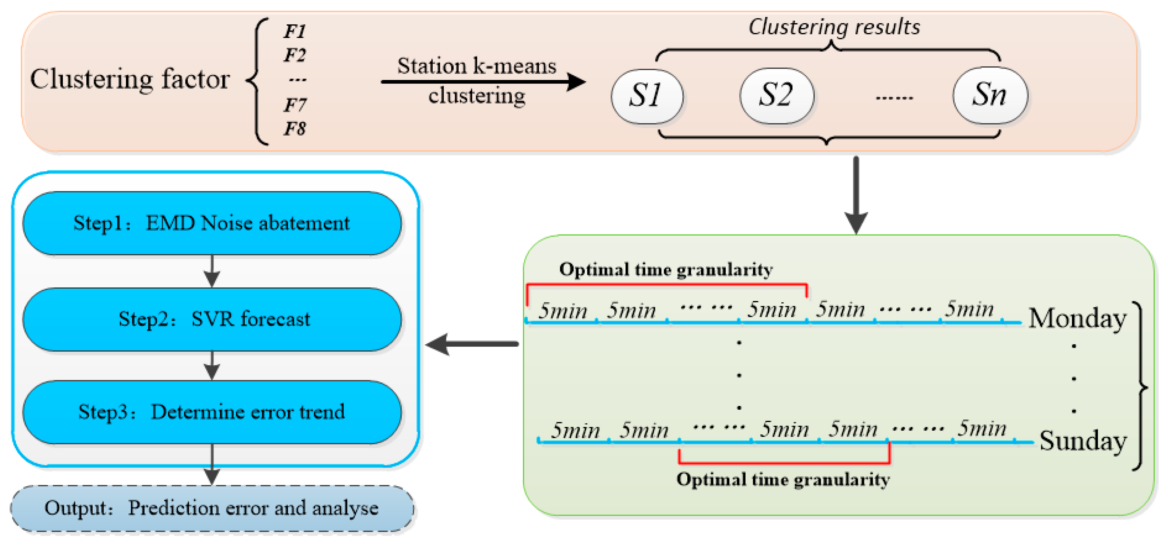
- The metro stations are classified by the changing law of passenger flow as the influencing factors of station clustering. When the stations are classified into four categories, the effect of classification results are in good agreement with reality. According to the proportion of clustering factors, the stations can be defined as severe residential stations, mild residential stations, consumption, tourism and passenger transport terminal stations, and working stations. The classification results are in accordance with the actual situation.
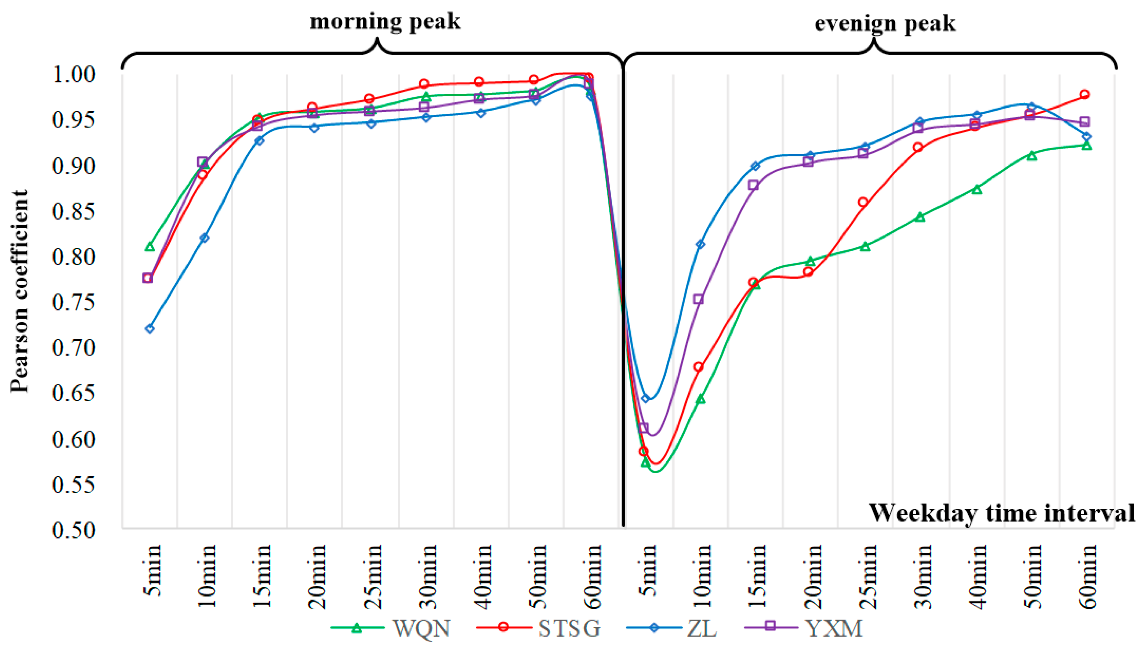
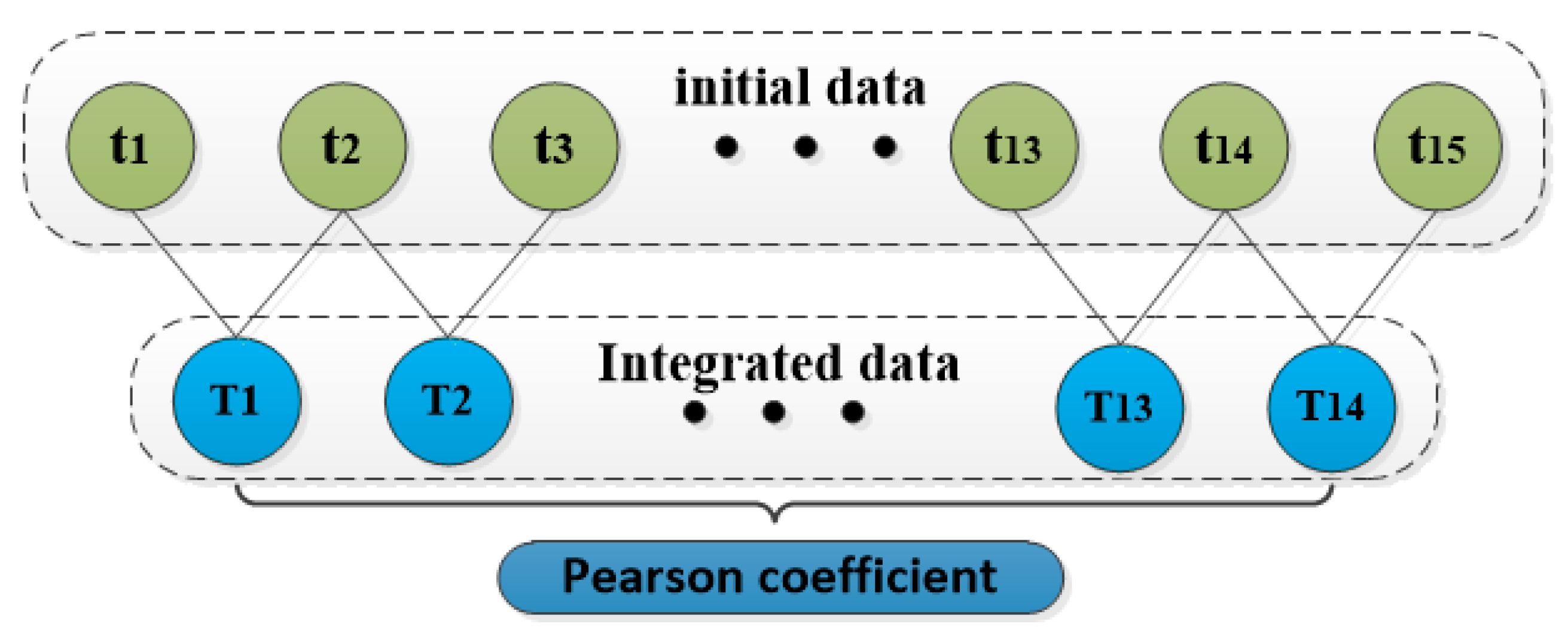
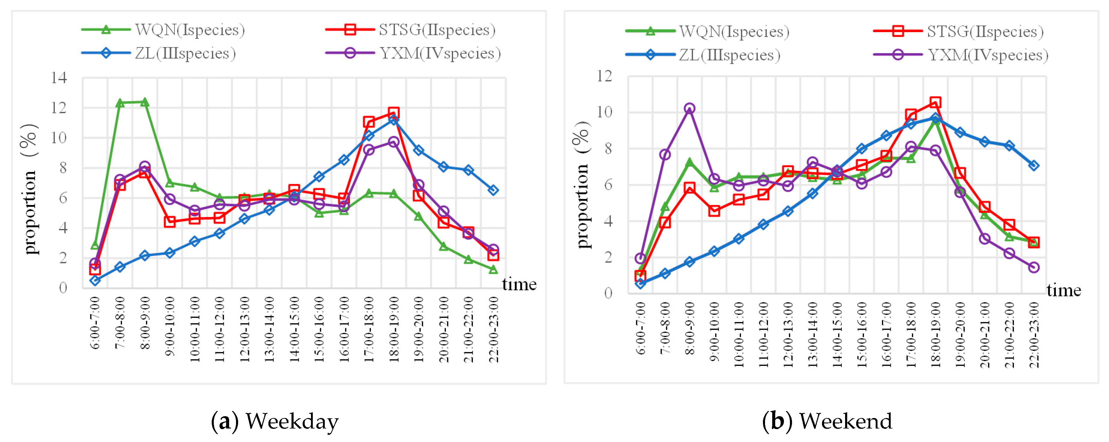
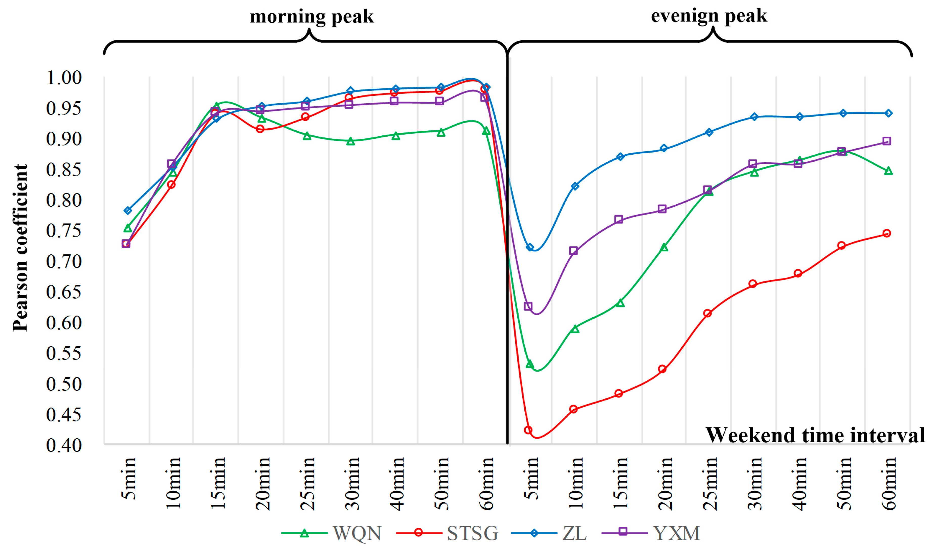
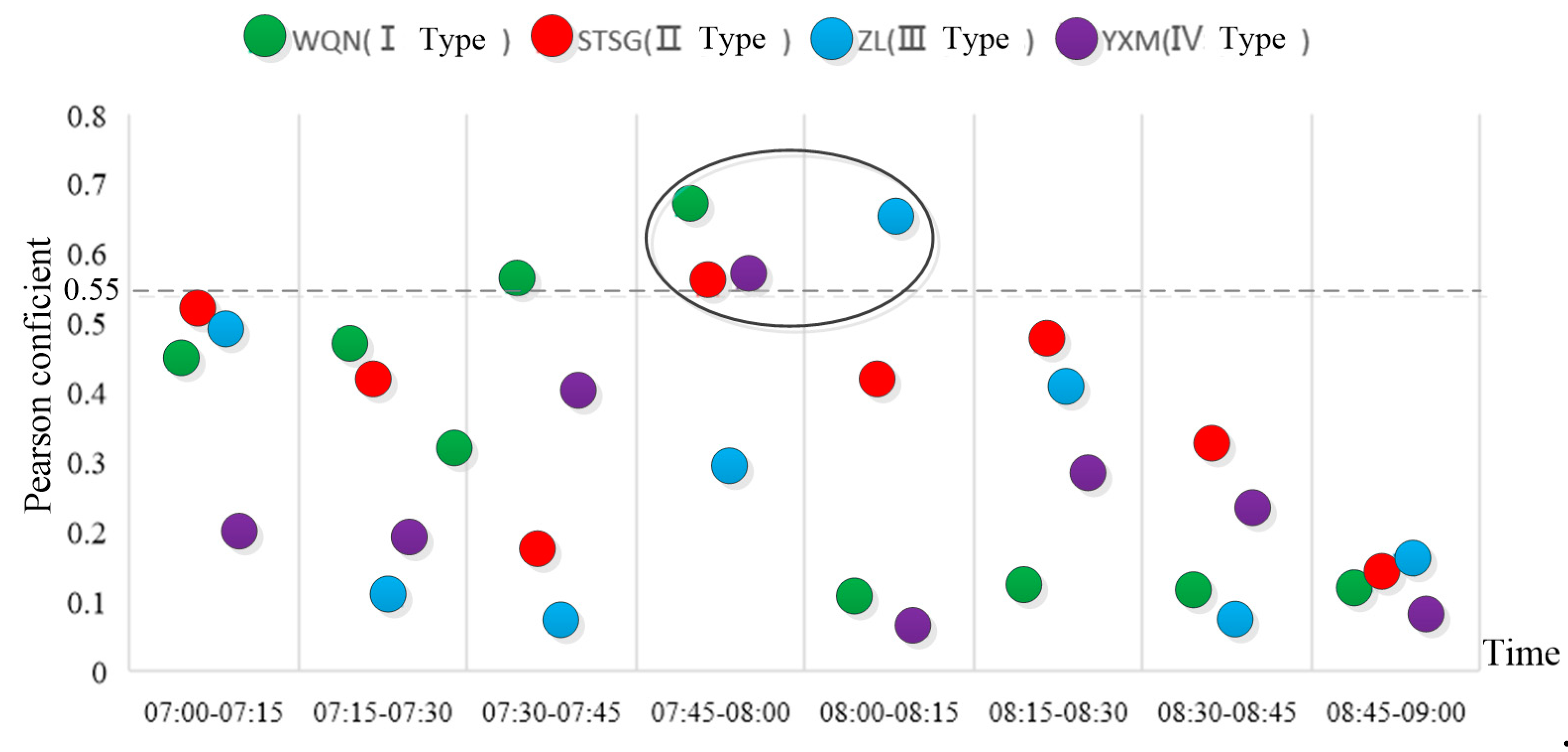
- The proportion of passenger flow varied from different time periods in different days of the week was analyzed, and the most practical time study range was determined. The improved Pearson coefficient method was used to determine the optimal time granularity of different types of stations. The range of predicted time: type I, II, and IV stations are 07:45–08:00 on weekdays, and type III stations are 08:00–08:15 on weekdays.
- An EMD-SVR prediction method is proposed. The advantage of this prediction method lies in the effective de-noising of prior data, which not only ensures the removal of white noise in time series, but also effectively preserves the characteristics of its own data variation law. The prediction results are compared with the traditional ARIMA, SVR, and BPNN methods, when the accuracy is improved to varying degrees.
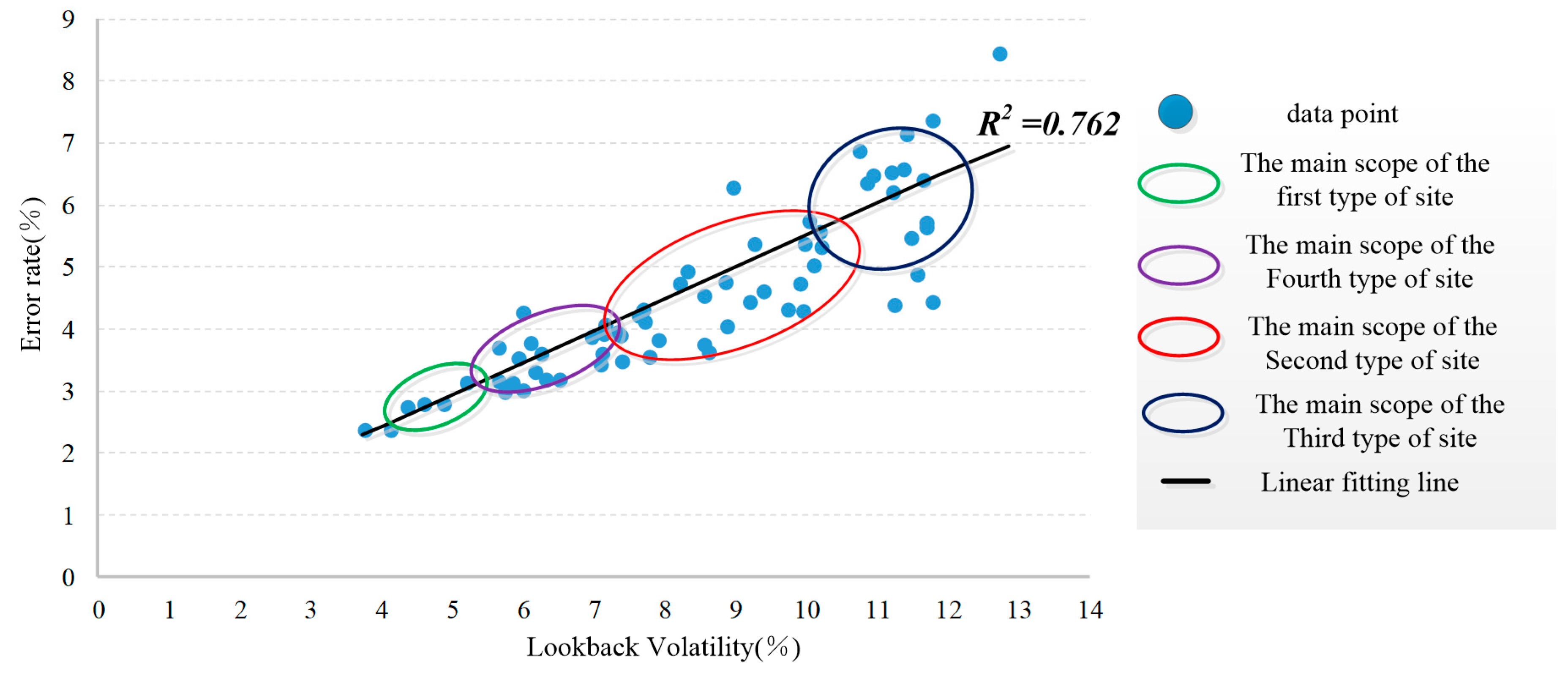
- After the selection and processing of the original data, the prediction accuracy of the four types of stations is different. The average prediction error of the four types of stations is 3.12%, 4.21%, 6.39%, and 3.79%, respectively. The fluctuation of passenger flow data is measured by LBV index, and the prediction error of 66 stations in the whole network is linearly fitted with LBV, and the R2 is 0.762.
Author Contributions
Funding
Acknowledgments
Conflicts of Interest
References
- Delgado, F.; Munoz, J.C.; Giesen, R. How much can holding and/or limiting boarding improve transit performance. Transp. Res. Part B Methodol. 2012, 46, 1202–1217. [Google Scholar] [CrossRef]
- Hernandez, D.; Munoz, J.C.; Giesen, R.; Delgado, F. Analysis of real-time control strategies in a corridor with multiple bus services. Transp. Res. Part B Methodol. 2015, 78, 83–105. [Google Scholar] [CrossRef]
- Williams, B.M. Multivariate vehicular traffic flow prediction: Evaluation of ARIMAX modeling. Transp. Res. Board 2001, 1776, 194–200. [Google Scholar] [CrossRef]
- Williams, B.M.; Hoel, L.A. Modeling and forecasting vehicular traffic flow as a seasonal ARIMA process: Theoretical basis and empirical results. J. Transp. Eng. 2003, 129, 664–672. [Google Scholar]
- Jiao, P.; Li, R.; Sun, T.; Hou, Z.; Ibrahim, A. Three Revised Kalman Filtering Models for Short-Term Rail Transit Passenger Flow Prediction. Math. Probl. Eng. 2016, 1–10. [Google Scholar] [CrossRef]
- Guo, J.; Huang, W.; Williams, B.M. Adaptive Kalman filter approach for stochastic short-term traffic flow rate prediction and uncertainty quantification. Transp. Res. Part C Emerg. Technol. 2014, 43, 50–64. [Google Scholar] [CrossRef]
- Li, R.M.; Lu, H.P. Combined Neural Network Approach for Short-Term Urban Freeway Traffic Flow Prediction. In Advances in Neural Networks—Isnn 2009; Yu, W., He, H.B., Zhang, N., Eds.; Springer: Berlin/Heidelberg, Germany, 2009; pp. 1017–1025. [Google Scholar]
- Bai, Y.; Sun, Z.; Zeng, B.; Deng, J.; Li, C. A multi-pattern deep fusion model for short-term bus passenger flow forecasting. Appl. Soft Comput. 2017, 58, 669–680. [Google Scholar] [CrossRef]
- Williams, N.; Zander, S.; Armitage, G. A preliminary performance comparison of five machine learning algorithms for practical IP traffic flow classification. Comput. Commun. Rev. 2006, 36, 7–15. [Google Scholar]
- Evgeniou, T.; Pontil, M.; Poggio, T. Regularization networks and support vector machines. Adv. Comput. Math. 2000, 13, 1–50. [Google Scholar] [CrossRef]
- Jeong, Y.S.; Byon, Y.J.; Castro-Neto, M.M.; Easa, S.M. Supervised Weighting-Online Learning Algorithm for Short-Term Traffic Flow Prediction. IEEE Trans. Intell. Transp. Syst. 2013, 14, 1700–1707. [Google Scholar] [CrossRef]
- Erfani, S.M.; Rajasegarar, S.; Karunasekera, S.; Leckie, C. High-dimensional and large-scale anomaly detection using a linear one-class SVM with deep learning. Pattern Recognit. 2016, 58, 121–134. [Google Scholar] [CrossRef]
- Balasubramanian, V.N. Deep Learning Advanced Computing and Communication. 2016 22nd Annual International Conference on Advanced Computing and Communication (ADCOM). Proceedings 2016. [Google Scholar] [CrossRef]
- Wu, Y.; Tan, H.; Qin, L.; Ran, B.; Jiang, Z. A hybrid deep learning based traffic flow prediction method and its understanding. Transp. Res. Part C Emerg. Technol. 2018, 90, 166–180. [Google Scholar] [CrossRef]
- Polson, N.G.; Sokolov, V.O. Deep learning for short-term traffic flow prediction. Transp. Res. Part C Emerg. Technol. 2017, 79, 1–17. [Google Scholar] [CrossRef] [Green Version]
- Zhang, W.; Chen, F.; Wang, Z. Similarity Measurement of Metro Travel Rules Based on Multi-time Granularities. J. China Railw. Soc. 2018, 40, 9–17. [Google Scholar]
- Ma, Z.L.; Xing, J.P.; Mesbah, M.; Ferreira, L. Predicting short-term bus passenger demand using a pattern hybrid approach. Transp. Res. Part C Emerg. Technol. 2014, 39, 148–163. [Google Scholar] [CrossRef]
- Shan, H.; Sadek, A.W. A novel forecasting approach inspired by human memory: The example of short-term traffic volume forecasting. Transp. Res. Part C Emerg. Technol. 2009, 17, 510–525. [Google Scholar] [CrossRef]
- Xia, B.; Kong, F.Y.; Xie, S.Y. Passenger Flow Forecast of Urban Rail Transit Based on Support Vector Regression. In Advances in Mechatronics and Control Engineering Ii, Pts 1-3; Galkowski, K., Kim, Y.H., Eds.; Trans Tech Publications: Fredericksburg, VA, USA, 2013; pp. 612–616. [Google Scholar]
- Zhong, C.; Batty, M.; Manley, E.; Wang, J.; Wang, Z.; Chen, F.; Schmitt, G. Variability in Regularity: Mining Temporal Mobility Patterns in London, Singapore and Beijing Using Smart-Card Data. PLoS ONE 2016, 11. [Google Scholar] [CrossRef]
- Sun, Y.X.; Leng, B.; Guan, W. A novel wavelet-SVM short-time passenger flow prediction in Beijing metro system. Neurocomputing 2015, 166, 109–121. [Google Scholar] [CrossRef]
- Utsunomiya, M.; Attanucci, J.; Wilson, N. Potential uses of transit smart card registration and transaction data to improve transit planning. Transp. Res. Rec. 2006, 1971, 118–126. [Google Scholar] [CrossRef]
- Ma, X.L.; Wu, Y.J.; Wang, Y.H.; Chen, F.; Liu, J.F. Mining smart card data for transit riders’ travel patterns. Transp. Res. Part C Emerg. Technol. 2013, 36, 1–12. [Google Scholar] [CrossRef]
- Wang, W.L.; Lo, S.M.; Liu, S.B. Aggregated Metro Trip Patterns in Urban Areas of Hong Kong: Evidence from Automatic Fare Collection Records. J. Urban Plan. Dev. 2015, 141. [Google Scholar] [CrossRef]
- Kim, M.K.; Kim, S.P.; Heo, J.; Sohn, H.G. Ridership patterns at metro stations of Seoul capital area and characteristics of station influence area. Ksce J. Civ. Eng. 2017, 21, 964–975. [Google Scholar] [CrossRef]
- Yu, L.; Chen, Q.; Chen, K. Deviation of Peak Hours for Urban Rail Transit Stations: A Case Study in Xi’an, China. Sustainability 2019, 11, 2733. [Google Scholar] [CrossRef]
- Liu, Y.; Liu, Z.; Jia, R. DeepPF: A deep learning based architecture for metro passenger flow prediction. Transp. Res. Part C Emerg. Technol. 2019, 101, 18–34. [Google Scholar] [CrossRef]
- Kouhi Esfahani, R.; Shahbazi, F.; Akbarzadeh, M. Three-phase classification of an uninterrupted traffic flow: A k-means clustering study. Transp. B Transp. Dyn. 2018, 7, 546–558. [Google Scholar] [CrossRef]
- Wei, Y.; Chen, M.-C. Forecasting the short-term metro passenger flow with empirical mode decomposition and neural networks. Transp. Res. Part C Emerg. Technol. 2012, 21, 148–162. [Google Scholar] [CrossRef]
- Du Yuchuan, S.Y. CHEN Ganzhe, Time granularity selection for expressway OD realtime prediction. J. Tongji Univ. 2016, 44, 1553–1558. [Google Scholar]
- Zwillinger, D.K. Stephen, Standard Probability and Statistics Tables and Formulae. Technometrics 2001, 43, 249–250. [Google Scholar] [CrossRef]
- Sun, S.; Zhang, C. The Selective Random Subspace Predictor for Traffic Flow Forecasting. IEEE Trans. Intell. Transp. Syst. 2007, 8, 367–373. [Google Scholar] [CrossRef]
- Huang, N.E.; Shen, Z.; Long, S.R.; Wu, M.C. The empirical mode decomposition and the Hilbert spectrum for nonlinear and non-stationary time series analysis. Proc. R. Soc. A Math. Phys. Eng. Sci. 1998, 454, 903–995. [Google Scholar] [CrossRef]


| Station Category | Number | F1 | F2 | F3 | F4 | F5 | F6 | F7 | F8 |
|---|---|---|---|---|---|---|---|---|---|
| I type | 5 | 0.110 | 0.650 | 0.879 | 0.109 | 0.400 | 0.421 | 1.924 | 1.89 |
| II type | 50 | 0.174 | 0.104 | 0.100 | 0.138 | 0.378 | 0.341 | 1.049 | 1.07 |
| III type | 14 | 0.111 | 0.090 | 0.101 | 0.114 | 0.394 | 0.387 | 1.135 | 1.330 |
| IV type | 18 | 0.111 | 0.161 | 0.134 | 0.097 | 0.387 | 0.370 | 0.855 | 0.930 |
| Station (Number) | Cluster | Station (Number) | Cluster | Station (Number) | Cluster | |||
|---|---|---|---|---|---|---|---|---|
| Class | Distance | Class | Distance | Class | Distance | |||
| HWZ(#1) | III | 0.093 | SQ(#2) | I | 0.078 | ZH(#3) | I | 0.124 |
| ZY(#4) | I | 0.095 | HCL(#5) | I | 0.179 | KYM(#6) | I | 0.128 |
| LDL(#7) | I | 0.110 | YXM(#8) | IV | 0.084 | SJQ(#9) | I | 0.115 |
| WLK(#10) | III | 0.154 | CYM(#11) | I | 0.187 | KFL(#12) | IV | 0.288 |
| THM(#13) | I | 0.168 | WSL(#14) | I | 0.088 | CLP(#15) | I | 0.186 |
| CH(#16) | I | 0.183 | BP(#17) | III | 0.172 | FZC(#18) | I | 0.185 |
| BKZ(#19) | III | 0.175 | BY(#20) | I | 0.134 | YDGY(#21) | III | 0.148 |
| XZZX(#22) | I | 0.095 | FCWL(#23) | I | 0.125 | STSG(#24) | I | 0.090 |
| DMGX(#25) | I | 0.163 | LSY(#26) | I | 0.141 | AYM(#27) | I | 0.056 |
| BDJ(#28) | I | 0.181 | ZL(#29) | III | 0.045 | YNM(#30) | IV | 0.152 |
| NSM(#31) | IV | 0.084 | TYC(#32) | I | 0.169 | XZ(#33) | III | 0.403 |
| WYJ(#34) | I | 0.062 | HZZX(#35) | I | 0.076 | SY(#36) | III | 0.193 |
| FXY(#37) | I | 0.183 | HTC(#38) | III | 0.137 | WQN(#39) | II | 0.099 |
| YHZ(#40) | I | 0.148 | ZBBL(#41) | I | 0.232 | YPM(#42) | IV | 0.240 |
| KJL(#43) | IV | 0.269 | TBNL(#44) | IV | 0.150 | JXC(#45) | IV | 0.116 |
| DYT(#46) | III | 0.309 | BCT(#47) | IV | 0.212 | QLS(#48) | I | 0.080 |
| YXM(#49) | I | 0.098 | XNL(#50) | III | 0.086 | CLGY(#51) | I | 0.101 |
| HJM(#52) | I | 0.201 | SJJ(#53) | I | 0.137 | XJM(#54) | I | 0.147 |
| GTM(#55) | I | 0.159 | THT(#56) | I | 0.123 | CBZX(#57) | IV | 0.100 |
| XHW(#58) | II | 0.274 | WZ(#59) | II | 0.237 | GJGW(#60) | III | 0.218 |
| SZ(#61) | I | 0.094 | XZ(#62) | II | 0.308 | BSQ(#63) | III | 0.214 |
| HTXC(#64) | IV | 0.207 | HTDL(#65) | IV | 0.110 | SZDD(#66) | IV | 0.312 |
| DCAJ(#67) | I | 0.145 | FTL(#68) | I | 0.127 | HTDD(#69) | II | 0.122 |
| JHT(#70) | I | 0.115 | QJCX(#71) | I | 0.112 | DTFR(#72) | III | 0.213 |
| XAKJ(#73) | I | 0.279 | JZKJ(#74) | I | 0.168 | HPM(#75) | I | 0.121 |
| DCS(#76) | IV | 0.091 | HYD(#77) | III | 0.118 | DMG(#78) | IV | 0.150 |
| DMGB(#79) | I | 0.085 | YJZ(#80) | I | 0.106 | BHC(#81) | I | 0.111 |
| CQL(#82) | I | 0.167 | SZYY(#83) | IV | 0.133 | WJL(#84) | I | 0.152 |
| FCJL(#85) | I | 0.136 | FCSE(#86) | IV | 0.174 | YSL(#87) | IV | 0.133 |
| Station | Time | Forecast Error | RMSE | Station | Time | Forecast Error | RMSE |
|---|---|---|---|---|---|---|---|
| WQN (I Type) | 07:00–07:15 | 5.18% | 56.1 | STSG (II Type) | 07:00–07:15 | 6.42% | 41.2 |
| 07:15–07:30 | 5.72% | 42.1 | 07:15–07:30 | 7.66% | 32.7 | ||
| 07:30–07:45 | 4.71% | 61.2 | 07:30–07:45 | 7.33% | 33.4 | ||
| 07:45–08:00 | 3.41% | 41.7 | 07:45–08:00 | 6.23% | 27.6 | ||
| 08:00–08:15 | 4.24% | 44.9 | 08:00–08:15 | 6.44% | 22.3 | ||
| 08:15–08:30 | 6.22% | 53.4 | 08:15–08:30 | 6.72% | 32.9 | ||
| 08:30–08:45 | 4.32% | 42.3 | 08:30–08:45 | 7.23% | 28.5 | ||
| 08:45–09:00 | 4.82% | 34.1 | 08:45–09:00 | 7.14% | 22.7 | ||
| ZL (III Type) | 07:00–07:15 | 8.22% | 45.4 | YXM (IV Type) | 07:00–07:15 | 6.43% | 44.2 |
| 07:15–07:30 | 7.12% | 35.2 | 07:15–07:30 | 6.22% | 37.2 | ||
| 07:30–07:45 | 8.22% | 44.2 | 07:30–07:45 | 5.72% | 31.4 | ||
| 07:45–08:00 | 7.41% | 36.2 | 07:45–08:00 | 5.33% | 34.1 | ||
| 08:00–08:15 | 7.31% | 34.4 | 08:00–08:15 | 5.43% | 30.3 | ||
| 08:15–08:30 | 7.65% | 36.2 | 08:15–08:30 | 6.14% | 28.3 | ||
| 08:30–08:45 | 8.11% | 33.2 | 08:30–08:45 | 6.53% | 22.1 | ||
| 08:45–09:00 | 7.54% | 37.4 | 08:45–09:00 | 5.44% | 27.4 |
| Station | Error | EMD-SVR | SVR | ARIMA | BPNN | Station | Error | EMD-SVR | SVR | ARIMA | BPNN |
|---|---|---|---|---|---|---|---|---|---|---|---|
| WQN | MAE | 29.4 | 38.7 | 33.8 | 56.4 | STSG | MAE | 13.1 | 24.4 | 15.7 | 28.9 |
| λ (%) | 3.16 | 4.53 | 3.41 | 4.42 | λ (%) | 5.66 | 8.43 | 6.23 | 8.87 | ||
| RMSE | 46.4 | 62.5 | 52.4 | 82.7 | RMSE | 22.1 | 35.4 | 22.3 | 40.2 | ||
| ZL | MAE | 22.5 | 33.2 | 21.7 | 38.6 | YXM | MAE | 17.2 | 26.6 | 19.3 | 27.2 |
| λ (%) | 6.12 | 9.23 | 7.31 | 8.22 | λ (%) | 4.88 | 7.33 | 5.33 | 6.87 | ||
| RMSE | 32.2 | 48.3 | 34.4 | 57.3 | RMSE | 27.2 | 41.1 | 30.3 | 45.1 |
© 2019 by the authors. Licensee MDPI, Basel, Switzerland. This article is an open access article distributed under the terms and conditions of the Creative Commons Attribution (CC BY) license (http://creativecommons.org/licenses/by/4.0/).
Share and Cite
Li, P.; Ma, C.; Ning, J.; Wang, Y.; Zhu, C. Analysis of Prediction Accuracy under the Selection of Optimum Time Granularity in Different Metro Stations. Sustainability 2019, 11, 5281. https://doi.org/10.3390/su11195281
Li P, Ma C, Ning J, Wang Y, Zhu C. Analysis of Prediction Accuracy under the Selection of Optimum Time Granularity in Different Metro Stations. Sustainability. 2019; 11(19):5281. https://doi.org/10.3390/su11195281
Chicago/Turabian StyleLi, Peikun, Chaoqun Ma, Jing Ning, Yun Wang, and Caihua Zhu. 2019. "Analysis of Prediction Accuracy under the Selection of Optimum Time Granularity in Different Metro Stations" Sustainability 11, no. 19: 5281. https://doi.org/10.3390/su11195281
APA StyleLi, P., Ma, C., Ning, J., Wang, Y., & Zhu, C. (2019). Analysis of Prediction Accuracy under the Selection of Optimum Time Granularity in Different Metro Stations. Sustainability, 11(19), 5281. https://doi.org/10.3390/su11195281