Article

Analysis of Prediction Accuracy under the Selection of Optimum Time Granularity in Different Metro Stations

School of Highway, Chang’an University, Xi’an 710064, China
*
Author to whom correspondence should be addressed.
Sustainability 2019, 11(19), 5281; https://doi.org/10.3390/su11195281
Submission received: 29 August 2019 / Revised: 21 September 2019 / Accepted: 21 September 2019 / Published: 25 September 2019
(This article belongs to the Collection Sustainable Rail and Metro Systems)

Abstract

:
The improvement of accuracy of short-term passenger flow prediction plays a key role in the efficient and sustainable development of metro operation. The primary objective of this study is to explore the factors that influence prediction accuracy from time granularity and station class. An important aim of the study was also in presenting the proposition of change in a forecasting method. Passenger flow data from 87 Metro stations in Xi’an was collected and analyzed. A framework of short-term passenger flow based on the Empirical Mode Decomposition-Support Vector Regression (EMD-SVR) was proposed to predict passenger flow for different types of stations. Also, the relationship between the generation of passenger flow prediction error and passenger flow data was investigated. First, the metro network was classified into four categories by using eight clustering factors based on the characteristics of inbound passenger flow. Second, Pearson correlation coefficient was utilized to explore the time interval and time granularity for short-term passenger flow prediction. Third, the EMD-SVR was used to predict the passenger flow in the optimal time interval for each station. Results showed that the proposed approach has a significant improvement compared to the traditional passenger flow forecast approach. Lookback Volatility (LVB) was applied to reflect the fluctuation difference of passenger flow data, and the linear fitting of prediction error was conducted. The goodness-of-fit (R2) was found to be 0.768, indicating a good fitting of the data. Furthermore, it revealed that there are obvious differences in the prediction error of the four kinds of stations.

1. Introduction

The rapid development of urban rail transit leads to the rapid growth of its passenger volume. However, capacity of the metro system could not meet the requirements of the large passenger flow. In order to ensure the sustainable development of rail transit, and to promote the development of the metro network passenger flow forecast, the refine development of metro passenger flow prediction has become a mainstream trend. Therefore, the prediction of short-time passenger flow plays an important role in metro operation management. It can provide the basis of control measures and technical support to the metro operation department, and adjustment of the operation organization [1,2].
In the aspect of short-term passenger flow prediction method, the autoregressive integrated moving average (ARIMA) model has been widely used because it does not need to consider the diversity of variables [3]. And WILLIAMS, et al. [4] proposed a SARIMA model by incorporating the influence of seasonal factors into the ARIMA model. On the other hand, Karman filtering model is applied to traffic flow prediction because it is not affected by its own data noise [5]. The variance invariance of the traditional Kalman filtering model process is improved, an adaptive Karman filter approach is provided, and the feasibility prediction is carried out by 15 min time granularity [6]. With the maturity of neural network technology, automatic adjustment of the neural network has also been applied to passenger flow prediction direction due to its own error feedback. A highway traffic flow prediction model based on the neural network has been proposed by Li and Lu [7]. The performance of the neural network model was verified by the measured data of Beijing third Ring Road Expressway. Based on the neural network model, a multi-pattern deep fusion (MPDF) method was proposed by Bai et al. [8] which classifies the passenger flow distribution of different clusters to adapt to different types of prediction models. In order to analyze nonlinear traffic data more effectively, machine learning was highlighted by its advantages of efficient self-training, which can avoid overtraining in neural networks [9,10]. An online learning weighted support vector regression model was proposed in short-term traffic passenger flow prediction based on the Support Vector Regression (SVR) model [11]. With the rapid development of computer technology, deep learning shows the ability to predict traffic flow under the background of big data [12,13]. Wu et al. [14] proposed a deep neural network capable of making full use of the temporal and spatial characteristics of traffic flow to improve prediction performance. Polson and Sokolov [15] proposed an end-to-end deep learning structure in metro passenger flow prediction.
The rationality of the prediction object and the validity of the prediction result should be fully considered to forecast the passenger flow. Moreover, the selection of time granularity is the basic issue in short-term passenger flow prediction, which affects the accuracy of the prediction results [16]. The Interactive Multi-Model based Pattern Hybrid (IMMPH) was developed to predict the bus passenger flow in three different time scales of week, day, and hour, respectively [17]. A spinning network (SPN) prediction method inspired by human memory was proposed to predict the number of road vehicles in 15 min and 30 min, respectively [18]. Xia et al. [19] established several kinds of passenger flow prediction methods for rail transit. The incoming quantity under different time granularity in different time periods of the whole day was selected as the data sample, which showed that the prediction accuracy of SVR model was high. Zhong et al. [20] studied the law of urban flow model based on intelligent traffic card data in three international cities; namely, London, Singapore, and Beijing, which was helpful to provide an analytical framework. Sun et al. [21] constructed a Wavelet-SVM model to predict the incoming and outgoing stations, and to transfer passenger flow of Beijing metro with a time granularity of 15 min, achieving satisfactory results.
To the authors’ best knowledge, most of the existing studies have been aimed to predict the overall passenger flow of a metro station or a metro line. In general, the change of prior passenger flow data is an important factor in determining the prediction accuracy. Thus, a lack of overall consideration of the whole subway network, a certain station prediction method, and the selection of prediction time granularity are not necessarily suitable for all types of stations. Due to the unsystematic study on the basic problems of research on the Prediction of the Passenger Flow, there is a gap in improving the prediction accuracy just by varying the prediction method. In order to explore the difference of the passenger flow prediction infrastructure system among the stations, the following problems need to be solved:
Question 1: Is it possible to predict short-term passenger flow for all stations? What is the reason for the difference in the error of passenger flow prediction results in different stations?
Question 2: Under which time granularity will the passenger flow show a strong regularity, and will this regular difference affect the accuracy of the final prediction results?
Question 3: Is it reasonable to adopt the same time granularity for all stations, or select different prediction time granularity for different stations?
Therefore, this study conducted a cluster analysis to classify the metro stations. Subsequently, the correlation of the prior passenger flow for different types of stations was explored. Finally, the difference of short-term passenger flow prediction for different types of stations was determined.
Many previous studies have been conducted in the selection of station clustering methods. It is a feasible research direction of station clustering analysis to classify stations by swiping credit cards and making different operation policies for different stations [22]. Ma et al. [23] presented a density-based spatial clustering of applications with noise (DBSCAN) algorithm and developed a data mining program which could obtain the time and space characteristics of the transaction data of the smart card. Wang et al. [24] used the smart card management system to study the difference between directional traffic in different periods of time, and divided the typical stations in Hong Kong into three categories. Based on the smart card payment system, Kim et al. [25] studied the passenger metro travel characteristics by K-means method, and the stations were divided into five types according to the land use properties around the metro. The results showed that there were obvious differences between the travel characteristics of Seoul metro stations and other related characteristics.
In the following section, the study area and data collection were showed. In Section 3, the methods of site classification and time granularity selection were systematically discussed. In Section 4, an improved method of passenger flow prediction is proposed. The prediction results were compared with other prediction methods, and the relation between the prediction error and the prediction data was investigated. Finally, in Section 5 the main conclusions are summarized.

2. Study Area and Data

2.1. Study Area

Xi’an, located in the hinterland of China, is the capital city of Shanxi Province. Moreover, Xi’an is an important cultural and educational city in China. By the end of 2018, the permanent population of Xi’an is more than 10 million, where the built area of the urban area has exceeded 700 square kilometers.
Cut off of data statistical time, there were 4 metro lines in Xi’an, namely: line 1, line 2, line 3, and line 4, with a total mileage of 126.35 km. There are 87 stations, including 6 transfer stations in Xi’an. The first metro line 2 was operated on September 16, 2011 and the last metro line 4 was operated on December 26, 2018, respectively. The passenger flow volume of the whole network reaches 3.1 million times every day, and the growing tendency is obvious. The passenger flow intensity of Xi’an ranks first in China in 2018.
Therefore, it is very necessary to establish an efficient early warning mechanism of metro passenger flow. This requires that the target of short-term ridership prediction should be attributed to keeping the highest forecasting accuracy as much as possible in the selection of shorter time granularity.

2.2. Data Acquisition and Preliminary Analysis

The data in this study was provided by Xi’an Metro Operation Company. The Automatic Fare Collection (AFC) system was used to collect the data from 87 stations from 1 January, 2019 to 15 March, 2019, a total of 74 all-day passenger inflow and outflow, with a minimum acquisition interval of 5 minutes collected.
In order to ensure the validity of the prior data of passenger flow prediction, the passenger flow prediction time granularity and the prediction target are selected from 7:00 am to 23:00 pm. The data of this stage consists of normal working days, general holidays, and statutory large-scale holidays (Chinese Spring Festival), which could reflect the difference of station passenger flow in different time periods, and provide a basis for the time selection of passenger flow prediction.
The following information is obtained through the preliminary analysis of the station entry passenger volume of all-day statistical time period of each station:
(1) The passenger flow data from Tuesday to Thursday at each station are more stable than those from the same period in the past. Monday and Friday are the first and the last day of the workday, so the passenger flow data will fluctuate over a certain period of time.
(2) The characteristics of the peak hours in the morning and the evening of each station have a certain deviation due to the land use of the surrounding areas. Yu et al. [26] found that there may be a deviation between station’s peak hours of the rail transit station and the peak hours of the city. For some stations, the highest passage flow does not occur in the city peak hours. The reason for this phenomenon is that the passenger flow of the station is determined by the land use of the surrounding areas. Under normal circumstances, the early peaks of metro stations that are relatively far from the urban area may appear earlier. This will provide a basis for the selection of the short-term passenger flow prediction time range.
(3) If the passenger flow data of one week is taken as a unit, as the number of units increases, the unit value will also increase. That is, the passenger flow of the metro shows a macro growth trend, which is significantly different from other prediction fields. Moreover, Liu, et al. [27] pointed out that most of the current passenger flow predictions are based on the latest time interval data and do not account for the two main characteristics of the time series: period and tendency. This also provides new ideas for subsequent prediction work.

3. Methodology

In the short-term passenger flow prediction of the metro station, we should first classify and process the metro station based on passenger flow characteristics, and then analyze the prior passenger flow data of each kind of station, including the analysis of passenger flow data in different weekdays of one week, as well as the difference and stability of passenger flow in different time periods of the same day. On this basis, the time period and time granularity that satisfy the passenger flow prediction conditions are selected. The core idea of this paper is to investigate the relationship between prediction error and prior data by using the improved passenger flow prediction method to predict passenger flow. The relationship diagram is shown in Figure 1:

3.1. Cluster Analysis of Station

3.1.1. K-means Clustering Method

K-means clustering method has a good effect on data partition, and is widely used in traffic data division [28]. The core idea is to update the discrete variable factor data to each clustering center iteratively, while the distance is used as the similarity index. Therefore, the given data is concentrated into K class, and the center of each class is obtained according to the mean value of all the values in the class, and each class is described by clustering center. The Euclidean distance is selected as the similarity index, and the clustering goal is to minimize the sum of squares of all kinds of clustering, which is expressed as follows:
J = k = 1 k i = 1 n x i u k 2
where uk is the center of each cluster, x i is the distance of a single sample from the cluster, k is the number of clusters into which the sample is divided, and n is the number of samples.
The sample iterates many times until the best clustering effect is obtained. The general steps of the algorithm are as follows:
Step 1: The "initial value" of N clustering centers is selected. In our research, select a point as the first initial cluster center point randomly, then select the point farthest from the point as the second initial cluster center point, and then select the point with the largest distance from the first two points as the third point, and so on, until the K initial cluster center points are selected.
Step 2: According to the principle of nearest distance from the center, all data points are assigned to the nearest center, thus all data are divided into N clusters.
Step 3: Within each cluster, the average values of all individuals are calculated as the new Euclidean distance center of each cluster.
Step 4: Repeat the above steps 2 and 3 until the ownership is unchanged, and the classification is completed.
When using k-means mean clustering, the determination of clustering number needs to be paid more attention. Different clustering numbers have great influence on the quality and degree of freedom of clustering results. In order to evaluate the strength of this effect, Silhouettes analysis is used to evaluate the quality of clustering effect. The definition of Silhouettes Coefficient is as follows:
s ( i ) = b ( i ) a ( i ) max { b ( i ) , a ( i ) }
where b(i) is the average distance between the sample and all points in the nearest cluster as the degree of separation with the nearest cluster, a(i) is the average distance of the same data from all other data in the same cluster. The value range of s(i) is from −1 to 1. When the degree of polymerization in the cluster is equal to the degree of separation, the contour coefficient is 0 and the contour coefficient is approximately 1. At this time, the clustering effect is the best. If the contour coefficient is negative, the sample is moved to the adjacent cluster, the contour coefficient of all the data is obtained, and the average contour coefficient of all the data can be obtained.

3.1.2. Selection of Clustering Factors

As the basis of short-term passenger flow prediction, passenger flow difference is the direct reason that affects the prediction results. As such, the selection of station classification clustering factors must also need passenger flow data difference as a support. In order to fully consider the station differences caused by passenger flow differences, eight clustering factors are selected as the factors of station clustering. It is worth noting that the selection of forecasting factors does not involve the impact of passenger flow quantity. The definitions of eight clustering factors are as follows:
(1) Workday morning peak hour entrance flow/workday full-time entrance flow (F1), workday morning peak hour exit flow/workday full-time exit flow (F2), workday evening peak hour entrance flow/workday full-time entrance flow (F3), workday evening peak hour exit flow/Workday full-time exit flow (F4). Through the data test, 7:30–8:30 is selected as the morning peak hour and 18:00–19:00 as the late peak time. The selection of this kind of factor can reflect the characteristics of passenger flow in the morning and evening of the station.
(2) Weekend entrance flow during 10:00–16:00/weekend full-time entrance flow (F5), weekend exit flow during 10:00–16:00/weekend full-time exit flow (F6). These kinds of factors reflect the station passenger flow characteristics during the non-peak hour.
(3) Weekend full-time entrance flow/workday full-time entrance flow (F7), Weekend full-time exit flow/workday full-time exit flow (F8). Such factors can reflect the differences in passenger flow between workdays and Weekends at various stations.

3.1.3. Case Analysis of Station Clustering

Up to the date of data statistics, there are 4 metro lines and 87 stations in Xi’an. In order to eliminate the influence of single data error on station classification, this paper takes the data from the station in Xi’an rail transit network as the research basis, and selects the three weeks from 11 February, 2019 to 3 March, 2019. After screening and sorting, a total of 8 clustering factors from F1 to F8 were extracted as the basis for station clustering. According to equation (2), when the clustering value k is 4, the contour coefficient has an elbow point, the classification effect is considered to be the best. the clustering factor weights corresponding to each cluster center after clustering are shown in Table 1.
According to the difference of each clustering factor, the four types of stations in the above table are defined as follows:
(1) Severe residential stations (I Type): most of these stations are concentrated in the first and last stations of metro lines, the proportion of entrance flow at the morning peak is high, and the proportion of exit flow is small (F1, F2), whereas the proportion of entrance/exit flow at evening peak is on the contrary (F3, F4), and the entrance/exit flow on weekdays is higher than that on holidays, that is F7, and F8 factor is larger. This kind of station is dominated by daily commuting passenger flow, so it is defined as a severe residential station.
(2) Mild residential station (II Type): the number of such stations is the largest, the main function is still residential, but it has both commercial and commercial functions. From Table 1, it can be seen that the proportion of the weight of morning and evening peak factors is more severe than that of residential stations.
(3) Consumption, tourism, and passenger terminal stations (III Type): the passenger flow characteristics of such stations are consistent with the characteristics of general consumption, tourism, and transportation hubs.
(4) Business work stations (IV Type): The characteristics and weight ratio of morning and evening peak and holiday passenger flow in this kind of station are contrary to the passenger flow characteristics and weight ratio of residential station. Considering that there are more commercial and official land around this kind of station, it is divided into a commercial work station.
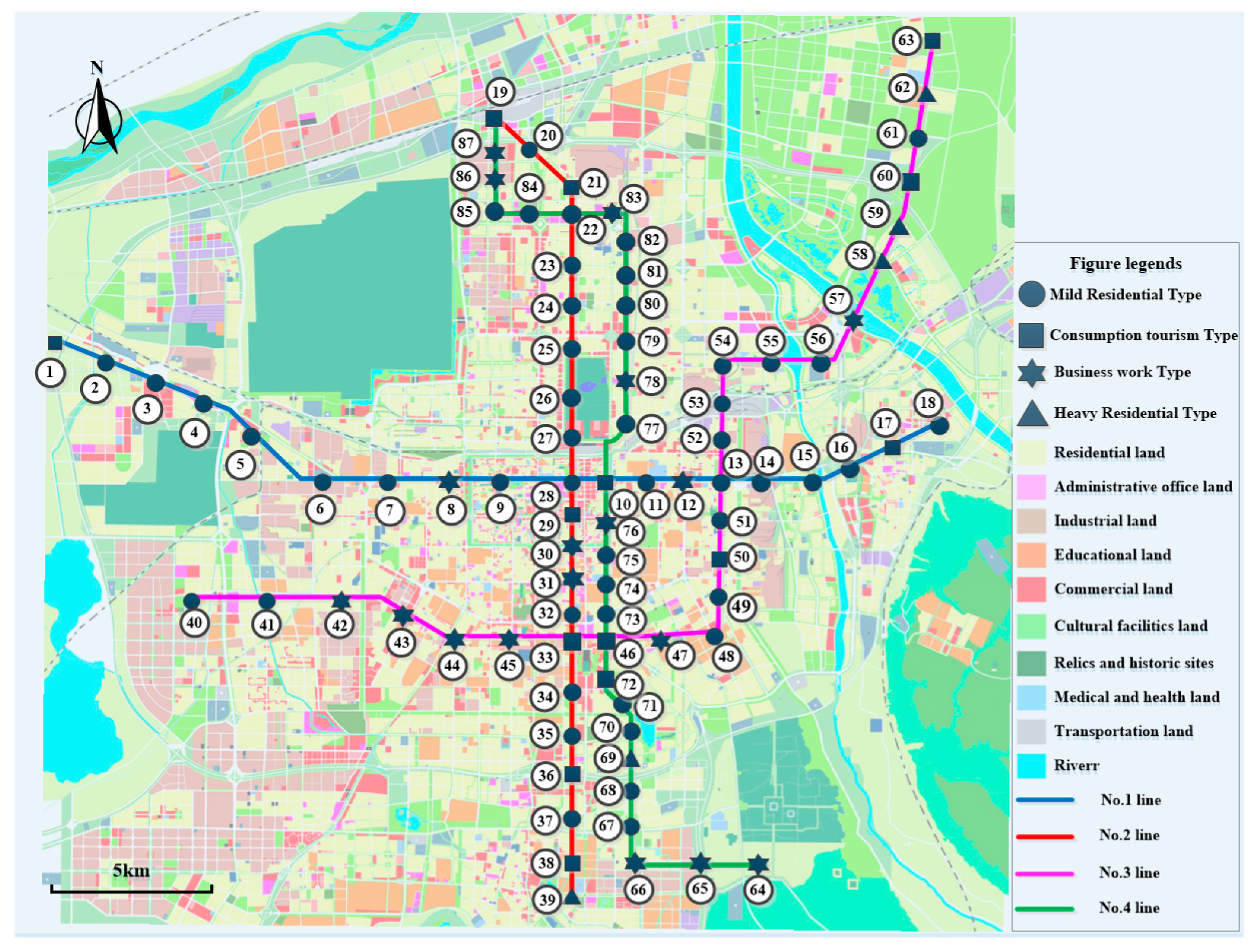
Table 2 shows the cluster types of 87 stations and the distance from the cluster centers. Figure 2 shows the relationship between the spatial location of stations and the type of stations more intuitively.

3.2. Time Granularity Study

3.2.1. Selection Range of Time Granularity

We should know that the significance of short-term passenger flow prediction is to guarantee the service level of passengers. The most direct influencing factor is queue waiting time. Therefore, for each station, when the passenger flow is the largest, making the most accurate passenger flow prediction with the smallest time granularity can provide technical support for the operation planning of the metro, and passengers can also have psychological expectations of the service level of the station [29]. In choosing the prediction period, we should consider the following question: Can we use the same time period to predict passenger flow for different types of stations? Is the determination of the time period related to workdays and holidays? In order to solve these two problems, we select the metro stations for a total of 21 days for three consecutive weeks to analyze the passenger flow law.
We choose four types of stations nearest to cluster center as the typical representatives of the above four types of stations for analysis. WQN is selected for the first type of station, STSG for the second type of station, ZL for the third type of station and YXM for the fourth type of station. Their distance from the center of their clusters can be obtained in Table 2. These four types of stations can effectively represent the difference of passenger flow characteristics of the four types of stations.
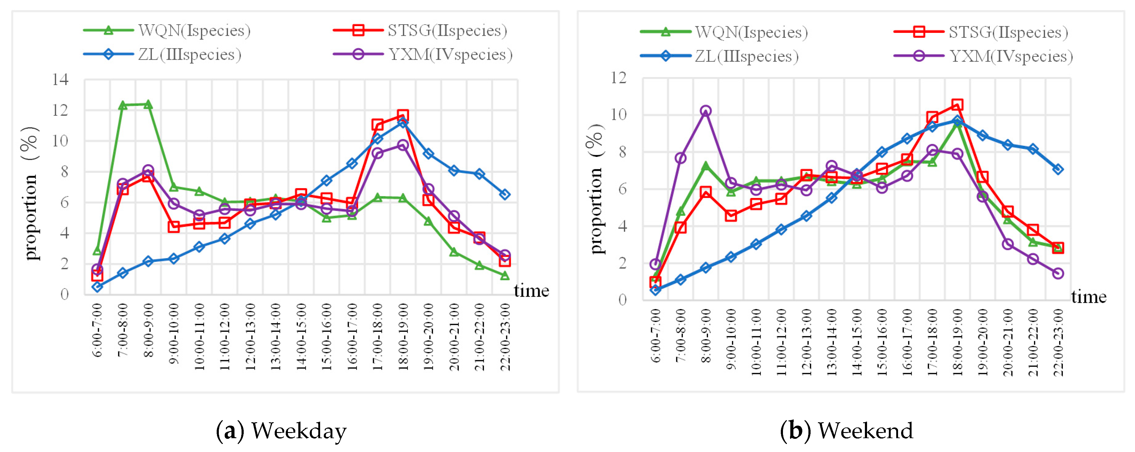
The effective operation time of Xi’an metro is determined to be a total of 17 hours from 06:00 to 23:00 for passenger flow analysis. Figure 3a indicates that the distribution of passenger flow in class I station during the workday shows a bimodal curve, and the proportion of morning peak passenger flow is at its highest during the day. The distribution of Type II and Type III of passenger flow also shows a bimodal phenomenon, and the proportion of passenger flow in the evening peak period is larger than the morning peak. The distribution curve of passenger flow in the IV type of station is unimodal, and the peak appears in the time range of 18:00–19:00. Figure 3b shows that the double peaks of the type I stations still exist in the holidays, but the proportion of passengers at the evening peaks exceeds the morning peaks. The passenger flow rate of the type II stations is close to that of the peak period; the type III stations are still unimodal. The change of passenger flow in the type IV station is similar to that of the type I station; that is, the morning and evening peak crossings are alternated. It can be seen from Table 2 that the distribution of passenger flow at the station is highly consistent with the station classification, and it is also consistent with other previous results on the changes of passenger flow in Xi’an metro in morning and evening peak hours [26].
Through the above analysis, and combined with the passenger flow to predict the actual demand, the short-term time granularity selection range is initially set to 7:00–9:00 and 18:00–19:00 for morning peak and evening peak, respectively.

3.2.2. Time Granularity Selection

To describe the station entrance passenger flow of station with an improved time series, the selected time period is divided into 9 time granularities for comparison: 5 min, 10 min, 15 min, 20 min, 25 min, 30 min, 40 min, 50 min, and 60 min:
X N = [ x 1 , 1 , x 1 , 2 , x 1 , 3 x 1 , n x 2 , 1 , x 2 , 2 , x 2 , 3 , x 2 , n x 27 , 1 , x 27 , 2 , x 27 , 3 , x 27 , n ]
where N is a sequence of consecutive days, N ∈ [1,27]; t ∈ (1,n), indicating that the effective morning operating hours of the metro lines are divided into n segments at time granularity Δt, n = 120/Δt (morning peak) or n = 60/Δt (evening peak).
Stationarity is an important feature of time series. The mean and variance of stationary time series will remain unchanged in the next period of time, while the unstable time series will produce large structural changes, which will weaken the accuracy and reliability of the prediction results [30]. Therefore, judging the stability of continuous time series data is an important step in the selection of time granularity. For data with continuity in time, Pearson correlation coefficient can discriminate the correlation between data [31]. For example: Sun and Zhang [32] indicated that the traffic flow data is incomplete and the data may be polluted by noise. The Pearson correlation coefficient is used to select the predicted input variables. The original data is extracted and the data similarity is measured by Pearson correlation coefficient method. It is assumed that the Pearson correlation coefficient r Δ t ( X i , X j ) with the granularity Δt of the time of day i and day j of the whole network is calculated as the coefficient between the row vector of row i and line j in XN, respectively. The calculation method is as follows.
r Δ t ( X i , X j ) = t = 1 n ( x N ( i ) t x N ( i ) ¯ ) ( x N ( j ) t x N ( j ) ¯ ) t = 1 n ( x N ( i ) t x N ( i ) ¯ ) 2 t = 1 n ( x N ( j ) t x N ( j ) ¯ ) 2
In the formula, XN(i)t represents the inbound amount in the t-th time period in the Nth day. x N ( i ) ¯ represents the average inbound of XN(i)t (N = 27). We divide the calculation process into weekdays and weekends, and in order to increase the accuracy of data similarity, we make j = i + 1; that is to say, the data of a certain period of a day is only compared with the same period of the next day, so that the data can be used more reasonably and effectively. If the coefficient is greater than zero, it means that there is a positive correlation between the entrance passenger flow for two consecutive days under the selected time granularity. If the coefficient is less than zero, it means that the two-time series show a negative correlation, which has no practical significance for the subsequent passenger flow prediction.
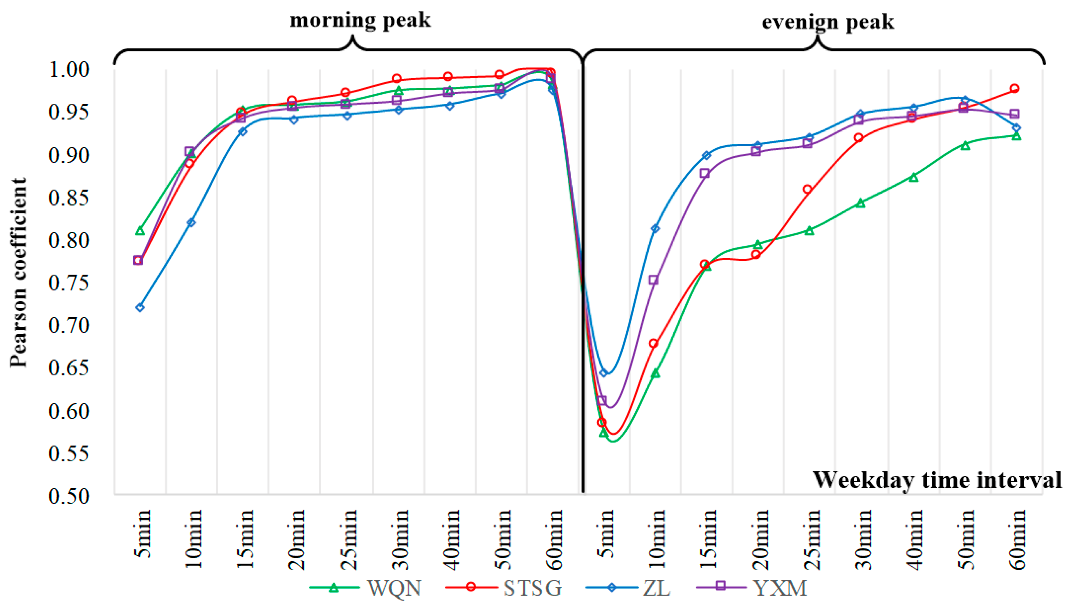
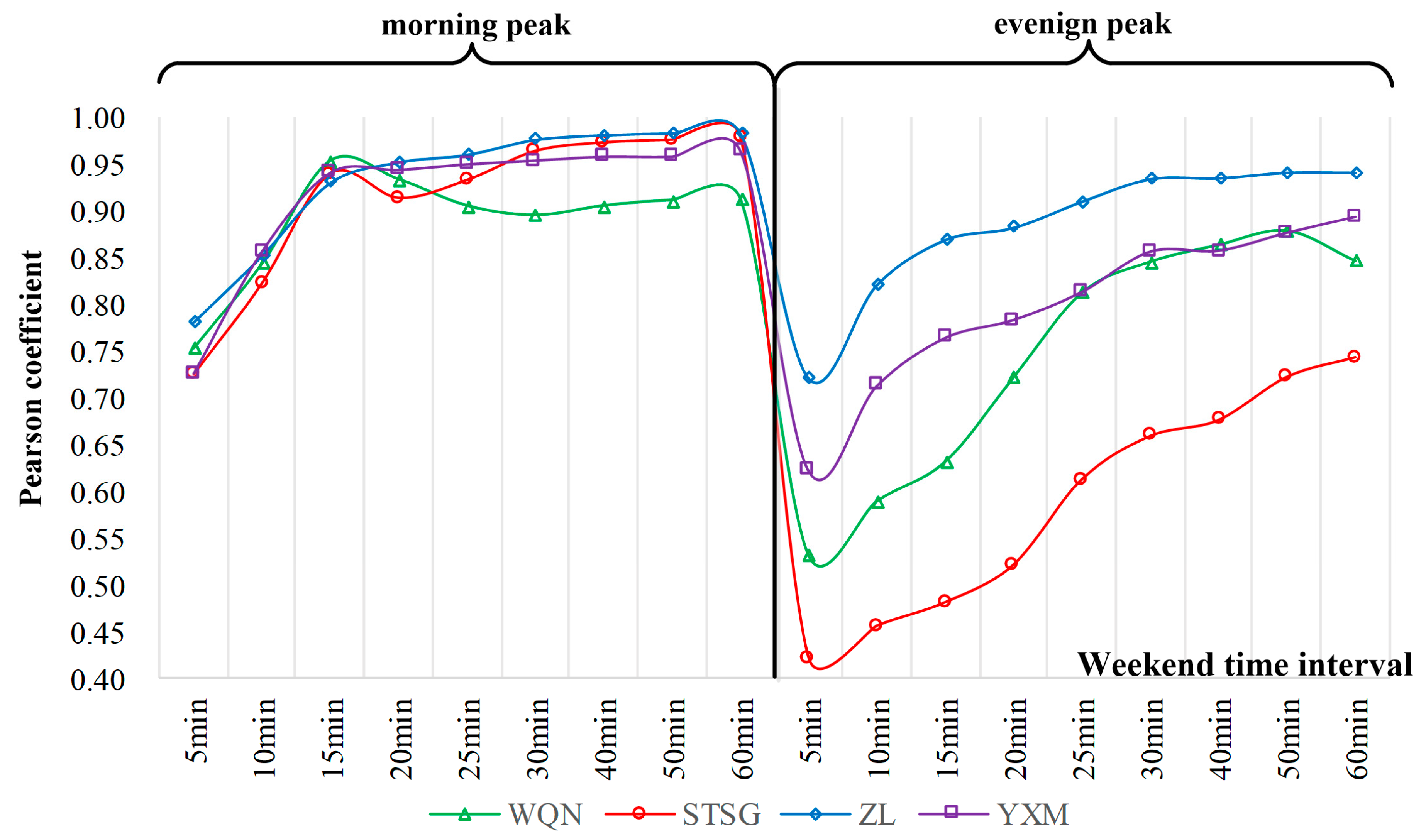
Figure 4 and Figure 5 show the Pearson correlations of the weekday and weekend, respectively. It can be concluded from the figures that no matter weekdays and weekends, the similarity coefficient of passenger flow increases with the increase of granularity from small to large during the early peak period. But it is worth noting that the growth rate of Pearson coefficient is faster in the process of increasing time granularity from 5 min to 15 min, and when the granularity continues to increase, the growth rate of Pearson coefficient slows down obviously. For the stations of I Type (WQN), standing at the morning peak of the holiday, when the time granularity increased to 15 min and then continued to increase, the similarity coefficient showed a certain degree of decline. For the evening peak, the correlation coefficient with the time granularity is basically the same as the early peak, except that the correlation coefficient at the same time granularity is lower than the early peak. The correlation coefficient at the same time granularity is higher in the workday than in the same time period of the weekend.

3.2.3. Selection Range of the Optimum Time Period

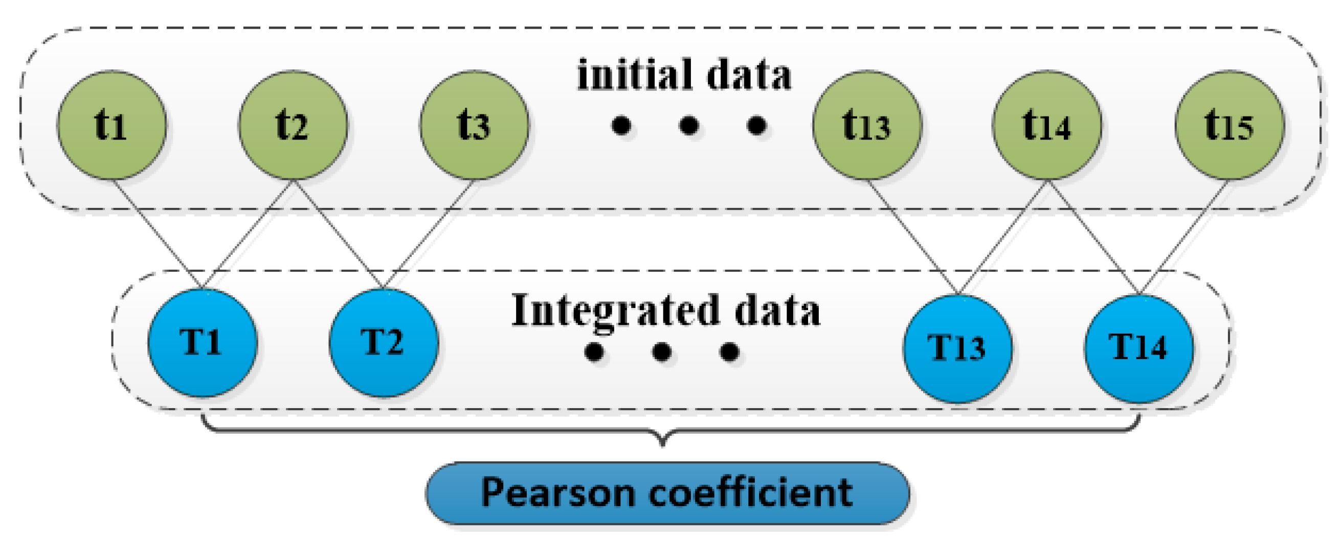
Through the above analysis, we determined that the 15 min time granularity of the four types of stations in the early peak hours of the workday is the sequence object of the passenger flow prediction, but we need to find out which period of 15-minute time has the greatest correlation with the arrival volume. Therefore, the 07:00–09:00 period is divided into eight periods for correlation comparison. Equation 4 is used for correlation coefficient comparison, but the selection of data is adjusted as follows: Taking the 8:00–8:15 time interval as an example, the data t1 of d1 day and the entrance passenger flow t2 of the same time interval of the adjacent working day d2 are selected as a new set of data T1, and then the data T2 is composed based on the data of day d2 and day d3. By analogy, 14 pairs of contrast data are generated in each time interval, and Pearson coefficients are calculated at last. Data consolidation process is shown in Figure 6.
It can be seen from Figure 7 that the regularity of passenger flow in the four types of stations presents different changes. 0.55 was selected as a threshold for the time period. The WQN station, STSG station and YXM station show the highest correlation at 07:45–08:00, and the correlation coefficient exceeds 0.55. Therefore, 07:45–08:00 time period is used as the best data selection time period for the passenger flow prediction of these three types of stations. Meanwhile, the maximum correlation of passenger flow at the ZL station appears at 08:00–08:15. Therefore, 08:00–08:15 time period is selected as the III Type station passenger flow prediction prior data.
In order to verify the validity of the time series selection of different types of stations, we use the (Autoregressive Integrated Moving Average) ARIMA model, which is more mature in passenger flow forecasting, to predict the eight time periods above. By using the ARIMA model to determine the closing and truncation criteria in the data autocorrelation and partial autocorrelation plots, WQN station selects ARIMA (1,1,2) model, STSG station and ZL station to select ARIMA (1,1,1) model. YXM station selects the ARIMA (2,1,3) model for prediction. In order to measure the magnitude of the prediction error, formula (5) and formula (6) are proposed to calculate the magnitude of the prediction error.
λ = 1 n i = 1 n | x i x i ¯ x i |
R M S E = 1 n i = 1 n ( x i ¯ x i ) 2
where, xi is the actual flow of the entrance of each station, x i ¯ is the predicted flow of the entrance of each station, the value of n is 49 and λ is the error value. This algorithm can accurately determine the prediction errors of different stations and different model methods, and provide data support for the subsequent error analysis. The prediction results of different types of sites using the ARIMA model are shown in Table 3.
It can be seen from Table 3 that the time period with less error of the four types of stations is directly related to the data correlation degree (the similarity coefficient of the time period with the smallest prediction error is higher), and the mean values of prediction errors are WQN (I Type), YXM (IV Type), STSG (II Type), ZL (III Type) in turn.

3.3. EMD-SVR Prediction Method

3.3.1. Process of Data De-noising

The composition of the metro passenger flow is complex and is always fluctuating, so it is difficult to strip off the noise influence of the predicted prior data because it is not determined whether the difference in the data is caused by an accidental difference or an empirically normal fluctuation. In order to solve the influence of data fluctuation on prediction results, EMD (empirical mode decomposition) is proposed to reduce data fluctuation caused by noise. EMD was originally proposed by E. Norden and Huang et al. [33]. It is a method for non-linear and non-stationary time series analysis. In this paper, the EMD method is used to perform the intrinsic mode function (IMF) reduction process on the data. The original data is subjected to first-order difference, and the smooth envelope defined by the local maximum and minimum values is selected based on the time series after the first-order difference. Then, the average of the envelopes is subtracted by the first-order differential time series. The value is obtained as a differential sequence after noise reduction, and finally the differential data is restored. First, the purpose of first-order difference is to find sufficient data extremum points to reduce the impact of raw data noise as comprehensively as possible. Second, it can ensure that the normal trend of data itself will not be too much subtracted in the process of noise reduction.
Δ y t = x t + 1 x t
where Δ y t represents the t phase value after the first order difference, xt+1 represents the original t+1 data, and xt represents the original t phase data.
F ( x n ) = f ( x n ) i = 1 n e x t Δ y n + e x t Δ y n + 1 2
where F(xn) denotes the n-phase sequence value after de-noising of the difference sequence, f(xn) represents the n-phase value of the difference sequence, and extΔyn is the n-th extreme value of the difference sequence. After obtaining the de-noised differential sequence and performing inverse difference, the original time series after noise reduction is obtained. Figure 8 shows a schematic diagram of the noise reduction using this method for the 15 min of a station.

3.3.2. SVR Model Prediction

Support Vector Machine (SVM) is a machine learning method for classification and nonlinear regression analysis. This method essentially avoids the traditional process from induction to deduction, and achieves a highly efficient method from training samples to forecasting samples. A small number of support vectors determine the final decision function. This feature not only helps researchers grasp key samples and eliminates a large number of redundant samples, but also makes the algorithm simple and has good "robustness". The principle is that: there is a training set { x i , y i } , x i R D (xi Contains class D vectors). For the problem of passenger flow prediction, the calculation formula of SVM objective function is defined in Equation (9) and (10).
min w , b = 1 2 w 2
s t y i ( w t x i + b ) 1 , i = 1 ,   2 m
where, w = (w1, w2, … wd) is the normal vector and b is the difference and determines the position of the hyperplane. The SVR uses a non-sensitive function ξ, which means that the objective function is considered to have no loss if the error range is within the acceptable range. If the error value is greater than ξ, calculate its loss minus ξ. Therefore, the SVR problem is converted to:
min w , b 1 2 w 2 + c i = 1 m l ξ ( f ( x i ) y i )
where c is a regularization parameter and is an insensitive function.

3.4. Prediction Result Analysis and Model Performance Comparision

3.4.1. Prediction Result Analysis

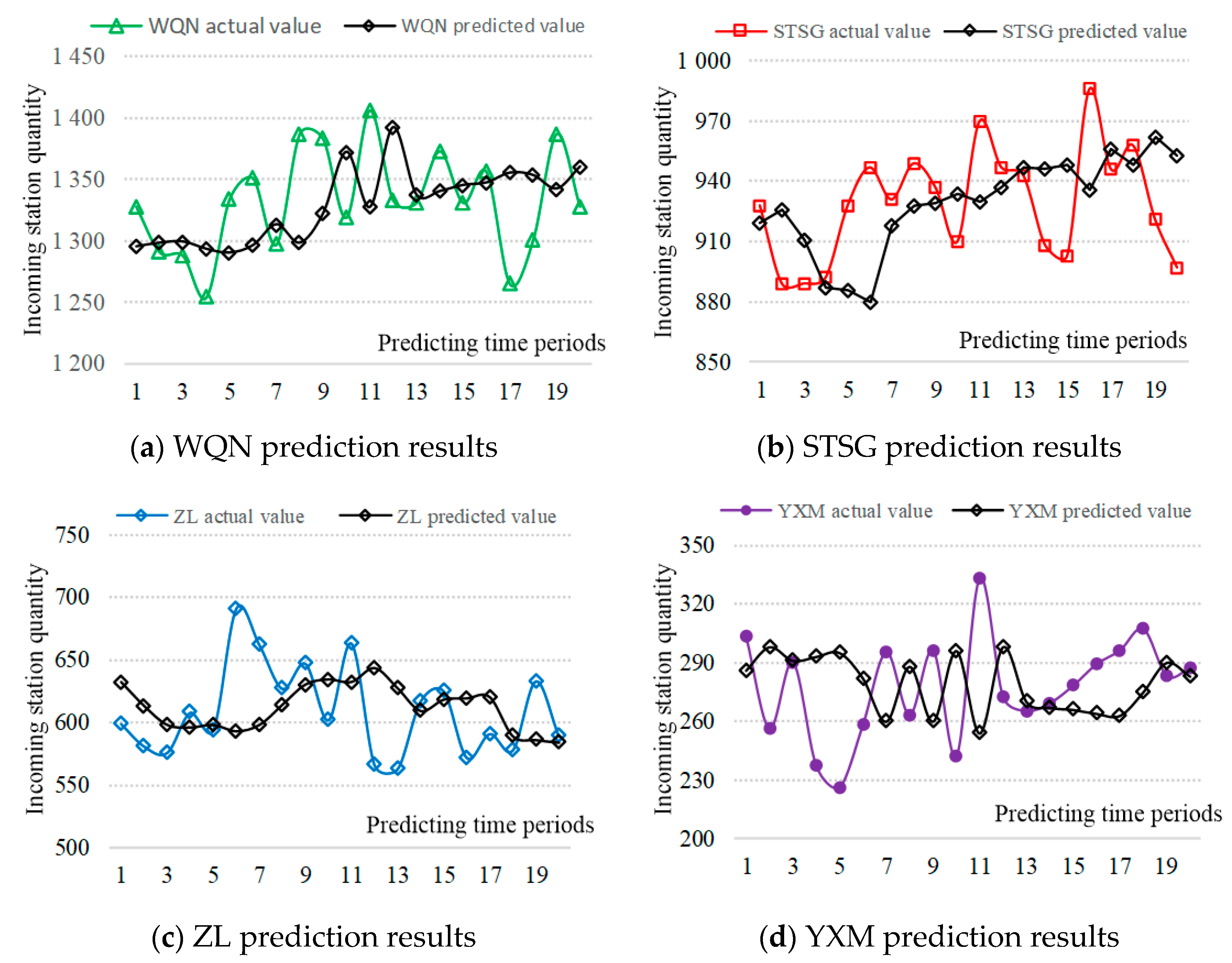
The data collected from each station from 1 January, 2019 to15 March, 2019 for 50 consecutive working days were used to forecast the entrance passenger flow. According to the working principle of SVR (Support Vector Regression) model, through the analysis of 50 data, it is found that the decision function obtained by training the first 30 data has relatively less errors in the prediction. The results are shown in Figure 9.
Based on the EMD-SVR method, the optimal time-granularity passenger flow of four representative stations in the optimal period of 50 consecutive working days is predicted. The actual value and the predicted value are shown in Figure 9. The actual value (the line indicated as color in the figure) fluctuates near the prediction line, indicating that the proposed method can predict the selected passenger flow data accurately.

3.4.2. BPNN Prediction Model Introduction

Back Propagation Neural Network (BPNN) is the most basic neural network, and its output uses forward propagation. The error is transmitted by back propagation. Structurally speaking, the BP network has an input layer, a hidden layer, and an output layer. In essence, the BP algorithm uses the square of the network error as the objective function and uses the gradient descent method to calculate the minimum value of the objective function.
The process of BP neural network is mainly divided into two stages. The first stage is the forward propagation of the signal, from the input layer through the hidden layer, and finally to the output layer. The second stage is the back propagation of the error, from the output layer to the hidden layer. The layer is included, and finally to the input layer, which adjusts the weight and offset of the hidden layer to the output layer, and the weight and offset of the input layer to the hidden layer.

3.4.3. Comparative Analysis of Predicting Results (EMD-SVR) and Other Methods

In order to verify the superiority of the EMD-SVR prediction method, the author considered SVR, ARIMA, and BPNN methods and assumed as comparative parameters MAE and RMSE. Moreover, the classical event sequence prediction method was compared under the same prior data conditions. The BPNN method parameters are set to 7 nodes in the input layer, 1 node in the output layer, 5 nodes in the hidden layer, a learning rate of 0.005, and a maximum number of iterations is 1000. The parameters of ARIMA model and SVR model are given in Section 3.2.3 and Section 3.4.1, respectively. Table 4 shows the comparison of prediction results at different sites.
From Table 4, we can know that when four kinds of prediction methods are used to predict four types of stations, the error and other prediction indicators are ranked in the same order. The prediction errors are from small to large, respectively: WQN (I Type), YXM (IV Type), STSG (II Type); The EMD-SVR method has a significant improvement over the other three methods, both in terms of prediction accuracy and other indicators.

4. Results and Analysis

We use different methods to predict, but get the same trend of prediction error. From this, we can infer that the difference of entrance passenger flow data of different types of stations is the root cause of this error trend. In order to find out how this difference affects the prediction results, Lookback Volatility (LBV) was used to describe the extent of passenger flow changes. Its definition is as follows:
b i = ln ( x i x i 1 )
μ = 1 n i = 2 n ( b i b ¯ ) 2
where xi is the entrance passenger flow of the i-th station; n is the number of data periods, and 20 is chosen here as the same amount of predicted data.
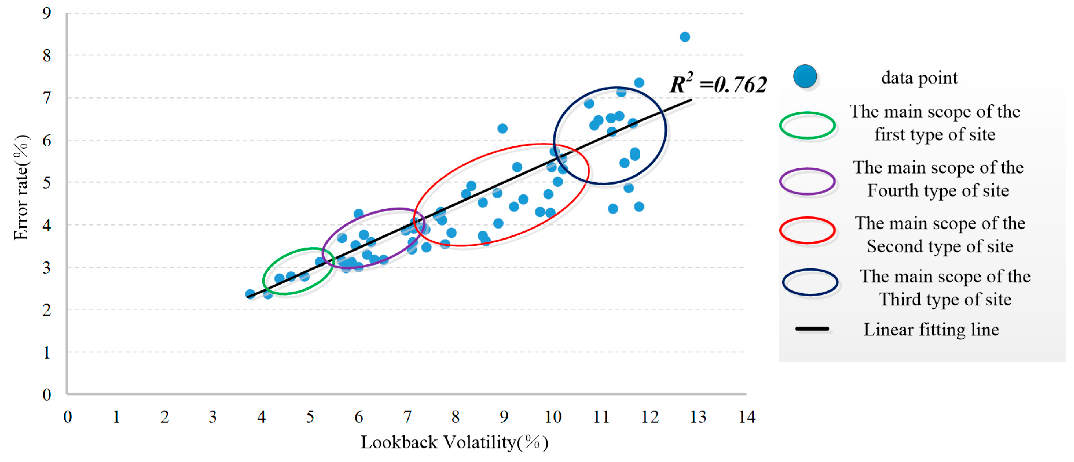
The calculated values of WQN, STSG, ZL, and YXM entry data are 4.618%, 6.713%, 9.835%, and 6.124%, respectively. The results show that there is a significant positive correlation between the magnitude of the lookback reverge value of each station and the fitting prediction error. In order to obtain as much data as possible for data fitting and minimize the impact of accidental errors, 21 stations with less than 100 in the optimum forecast period are excluded. The purpose of eliminating these stations is to ensure a better fitting effect. Finally, 66 stations are selected to analyze the relationship between the error of passenger flow model and the fluctuation of entrance passenger flow data. Figure 10 is a plot of the prediction error obtained by using the EMD-SVR model and the data look back volatility.
In the figure above, we linearly fit all the data points and found that there is a close relationship between the prediction error rate and LBV. If error rate is the dependent variable y and LBV is the independent variable x, then the relationship can be fitted to y = 0.498x+ 0.3053, and the R-square of the fitted linear equation reaches 0.762, indicating that the fitting effect is better. We also mark the location of different types of sites in the figure. The number of sites in the first type of circle accounts for 100% of the number of sites in the first category; the second category is 82.5%, and the third category is 72.7%. The fourth category is 75%. It shows that there are significant differences in prediction errors between different types of stations. The average prediction error of the I type stations is 3.12%, and the standard deviation is 0.402. The average prediction error of the II type stations is 4.21%, and the standard deviation is 1.242. The mean error of the III type stations is predicted. It is 6.39% with a standard deviation of 2.142; the average error of the IV type station is 3.64%, and the standard deviation is 1.252.

5. Conclusions

This paper takes Xi’an metro as the research object, classifies 87 metro stations in the whole network, and conducts research on the best time granularity and time period selection. On the basis of this, and by predicting the passenger flow of different types of stations, we have come to the following conclusions:
  • The metro stations are classified by the changing law of passenger flow as the influencing factors of station clustering. When the stations are classified into four categories, the effect of classification results are in good agreement with reality. According to the proportion of clustering factors, the stations can be defined as severe residential stations, mild residential stations, consumption, tourism and passenger transport terminal stations, and working stations. The classification results are in accordance with the actual situation.
  • The proportion of passenger flow varied from different time periods in different days of the week was analyzed, and the most practical time study range was determined. The improved Pearson coefficient method was used to determine the optimal time granularity of different types of stations. The range of predicted time: type I, II, and IV stations are 07:45–08:00 on weekdays, and type III stations are 08:00–08:15 on weekdays.
  • An EMD-SVR prediction method is proposed. The advantage of this prediction method lies in the effective de-noising of prior data, which not only ensures the removal of white noise in time series, but also effectively preserves the characteristics of its own data variation law. The prediction results are compared with the traditional ARIMA, SVR, and BPNN methods, when the accuracy is improved to varying degrees.
  • After the selection and processing of the original data, the prediction accuracy of the four types of stations is different. The average prediction error of the four types of stations is 3.12%, 4.21%, 6.39%, and 3.79%, respectively. The fluctuation of passenger flow data is measured by LBV index, and the prediction error of 66 stations in the whole network is linearly fitted with LBV, and the R2 is 0.762.
Through the error study of prediction accuracy, the relationship between error size and data fluctuation is determined. However, there are still many studies that need to be done in the future. First of all, the feasibility of prediction should be examined for large holidays (National Day holiday, Spring Festival, Mid-Autumn Festival, etc.), and no special holidays have been discussed in this paper. Secondly, for special stations, such as transfer stations, high-speed rail connection stations because of the particularity of their passenger flow sources, its passenger flow fluctuations are large, for this special station should be more detailed research, should not be limited to the accuracy of passenger flow prediction. Finally, this paper only considers the number of stations, but there are still many other factors affecting the service level of a station. In future work, the impact of outbound and transfer passenger flow on the station passenger flow should be considered. Meanwhile, the sudden change of station passenger volume caused by sudden bad conditions should also be taken into account.

Author Contributions

Conceptualization, P.L.; methodology, P.L.; software, J.N.; validation, P.L.; formal analysis, C.Z. and C.M.; investigation, P.L.; resources, C.M.; data curation, Y.W.; writing—original draft preparation, P.L. and C.Z; writing—review and editing, Y.W.; visualization, C.M.; funding acquisition, C.M.

Funding

This research was funded by the National Natural Science Foundation of China, grant number 71871027.

Acknowledgments

Here we acknowledge the anonymous reviewers and authors of cited papers for their detailed comments, without which this work would not have been possible.

Conflicts of Interest

The authors declare no conflict of interest.

References

  1. Delgado, F.; Munoz, J.C.; Giesen, R. How much can holding and/or limiting boarding improve transit performance. Transp. Res. Part B Methodol. 2012, 46, 1202–1217. [Google Scholar] [CrossRef]
  2. Hernandez, D.; Munoz, J.C.; Giesen, R.; Delgado, F. Analysis of real-time control strategies in a corridor with multiple bus services. Transp. Res. Part B Methodol. 2015, 78, 83–105. [Google Scholar] [CrossRef]
  3. Williams, B.M. Multivariate vehicular traffic flow prediction: Evaluation of ARIMAX modeling. Transp. Res. Board 2001, 1776, 194–200. [Google Scholar] [CrossRef]
  4. Williams, B.M.; Hoel, L.A. Modeling and forecasting vehicular traffic flow as a seasonal ARIMA process: Theoretical basis and empirical results. J. Transp. Eng. 2003, 129, 664–672. [Google Scholar]
  5. Jiao, P.; Li, R.; Sun, T.; Hou, Z.; Ibrahim, A. Three Revised Kalman Filtering Models for Short-Term Rail Transit Passenger Flow Prediction. Math. Probl. Eng. 2016, 1–10. [Google Scholar] [CrossRef]
  6. Guo, J.; Huang, W.; Williams, B.M. Adaptive Kalman filter approach for stochastic short-term traffic flow rate prediction and uncertainty quantification. Transp. Res. Part C Emerg. Technol. 2014, 43, 50–64. [Google Scholar] [CrossRef]
  7. Li, R.M.; Lu, H.P. Combined Neural Network Approach for Short-Term Urban Freeway Traffic Flow Prediction. In Advances in Neural Networks—Isnn 2009; Yu, W., He, H.B., Zhang, N., Eds.; Springer: Berlin/Heidelberg, Germany, 2009; pp. 1017–1025. [Google Scholar]
  8. Bai, Y.; Sun, Z.; Zeng, B.; Deng, J.; Li, C. A multi-pattern deep fusion model for short-term bus passenger flow forecasting. Appl. Soft Comput. 2017, 58, 669–680. [Google Scholar] [CrossRef]
  9. Williams, N.; Zander, S.; Armitage, G. A preliminary performance comparison of five machine learning algorithms for practical IP traffic flow classification. Comput. Commun. Rev. 2006, 36, 7–15. [Google Scholar]
  10. Evgeniou, T.; Pontil, M.; Poggio, T. Regularization networks and support vector machines. Adv. Comput. Math. 2000, 13, 1–50. [Google Scholar] [CrossRef]
  11. Jeong, Y.S.; Byon, Y.J.; Castro-Neto, M.M.; Easa, S.M. Supervised Weighting-Online Learning Algorithm for Short-Term Traffic Flow Prediction. IEEE Trans. Intell. Transp. Syst. 2013, 14, 1700–1707. [Google Scholar] [CrossRef]
  12. Erfani, S.M.; Rajasegarar, S.; Karunasekera, S.; Leckie, C. High-dimensional and large-scale anomaly detection using a linear one-class SVM with deep learning. Pattern Recognit. 2016, 58, 121–134. [Google Scholar] [CrossRef]
  13. Balasubramanian, V.N. Deep Learning Advanced Computing and Communication. 2016 22nd Annual International Conference on Advanced Computing and Communication (ADCOM). Proceedings 2016. [Google Scholar] [CrossRef]
  14. Wu, Y.; Tan, H.; Qin, L.; Ran, B.; Jiang, Z. A hybrid deep learning based traffic flow prediction method and its understanding. Transp. Res. Part C Emerg. Technol. 2018, 90, 166–180. [Google Scholar] [CrossRef]
  15. Polson, N.G.; Sokolov, V.O. Deep learning for short-term traffic flow prediction. Transp. Res. Part C Emerg. Technol. 2017, 79, 1–17. [Google Scholar] [CrossRef] [Green Version]
  16. Zhang, W.; Chen, F.; Wang, Z. Similarity Measurement of Metro Travel Rules Based on Multi-time Granularities. J. China Railw. Soc. 2018, 40, 9–17. [Google Scholar]
  17. Ma, Z.L.; Xing, J.P.; Mesbah, M.; Ferreira, L. Predicting short-term bus passenger demand using a pattern hybrid approach. Transp. Res. Part C Emerg. Technol. 2014, 39, 148–163. [Google Scholar] [CrossRef]
  18. Shan, H.; Sadek, A.W. A novel forecasting approach inspired by human memory: The example of short-term traffic volume forecasting. Transp. Res. Part C Emerg. Technol. 2009, 17, 510–525. [Google Scholar] [CrossRef]
  19. Xia, B.; Kong, F.Y.; Xie, S.Y. Passenger Flow Forecast of Urban Rail Transit Based on Support Vector Regression. In Advances in Mechatronics and Control Engineering Ii, Pts 1-3; Galkowski, K., Kim, Y.H., Eds.; Trans Tech Publications: Fredericksburg, VA, USA, 2013; pp. 612–616. [Google Scholar]
  20. Zhong, C.; Batty, M.; Manley, E.; Wang, J.; Wang, Z.; Chen, F.; Schmitt, G. Variability in Regularity: Mining Temporal Mobility Patterns in London, Singapore and Beijing Using Smart-Card Data. PLoS ONE 2016, 11. [Google Scholar] [CrossRef]
  21. Sun, Y.X.; Leng, B.; Guan, W. A novel wavelet-SVM short-time passenger flow prediction in Beijing metro system. Neurocomputing 2015, 166, 109–121. [Google Scholar] [CrossRef]
  22. Utsunomiya, M.; Attanucci, J.; Wilson, N. Potential uses of transit smart card registration and transaction data to improve transit planning. Transp. Res. Rec. 2006, 1971, 118–126. [Google Scholar] [CrossRef]
  23. Ma, X.L.; Wu, Y.J.; Wang, Y.H.; Chen, F.; Liu, J.F. Mining smart card data for transit riders’ travel patterns. Transp. Res. Part C Emerg. Technol. 2013, 36, 1–12. [Google Scholar] [CrossRef]
  24. Wang, W.L.; Lo, S.M.; Liu, S.B. Aggregated Metro Trip Patterns in Urban Areas of Hong Kong: Evidence from Automatic Fare Collection Records. J. Urban Plan. Dev. 2015, 141. [Google Scholar] [CrossRef]
  25. Kim, M.K.; Kim, S.P.; Heo, J.; Sohn, H.G. Ridership patterns at metro stations of Seoul capital area and characteristics of station influence area. Ksce J. Civ. Eng. 2017, 21, 964–975. [Google Scholar] [CrossRef]
  26. Yu, L.; Chen, Q.; Chen, K. Deviation of Peak Hours for Urban Rail Transit Stations: A Case Study in Xi’an, China. Sustainability 2019, 11, 2733. [Google Scholar] [CrossRef]
  27. Liu, Y.; Liu, Z.; Jia, R. DeepPF: A deep learning based architecture for metro passenger flow prediction. Transp. Res. Part C Emerg. Technol. 2019, 101, 18–34. [Google Scholar] [CrossRef]
  28. Kouhi Esfahani, R.; Shahbazi, F.; Akbarzadeh, M. Three-phase classification of an uninterrupted traffic flow: A k-means clustering study. Transp. B Transp. Dyn. 2018, 7, 546–558. [Google Scholar] [CrossRef]
  29. Wei, Y.; Chen, M.-C. Forecasting the short-term metro passenger flow with empirical mode decomposition and neural networks. Transp. Res. Part C Emerg. Technol. 2012, 21, 148–162. [Google Scholar] [CrossRef]
  30. Du Yuchuan, S.Y. CHEN Ganzhe, Time granularity selection for expressway OD realtime prediction. J. Tongji Univ. 2016, 44, 1553–1558. [Google Scholar]
  31. Zwillinger, D.K. Stephen, Standard Probability and Statistics Tables and Formulae. Technometrics 2001, 43, 249–250. [Google Scholar] [CrossRef]
  32. Sun, S.; Zhang, C. The Selective Random Subspace Predictor for Traffic Flow Forecasting. IEEE Trans. Intell. Transp. Syst. 2007, 8, 367–373. [Google Scholar] [CrossRef]
  33. Huang, N.E.; Shen, Z.; Long, S.R.; Wu, M.C. The empirical mode decomposition and the Hilbert spectrum for nonlinear and non-stationary time series analysis. Proc. R. Soc. A Math. Phys. Eng. Sci. 1998, 454, 903–995. [Google Scholar] [CrossRef]
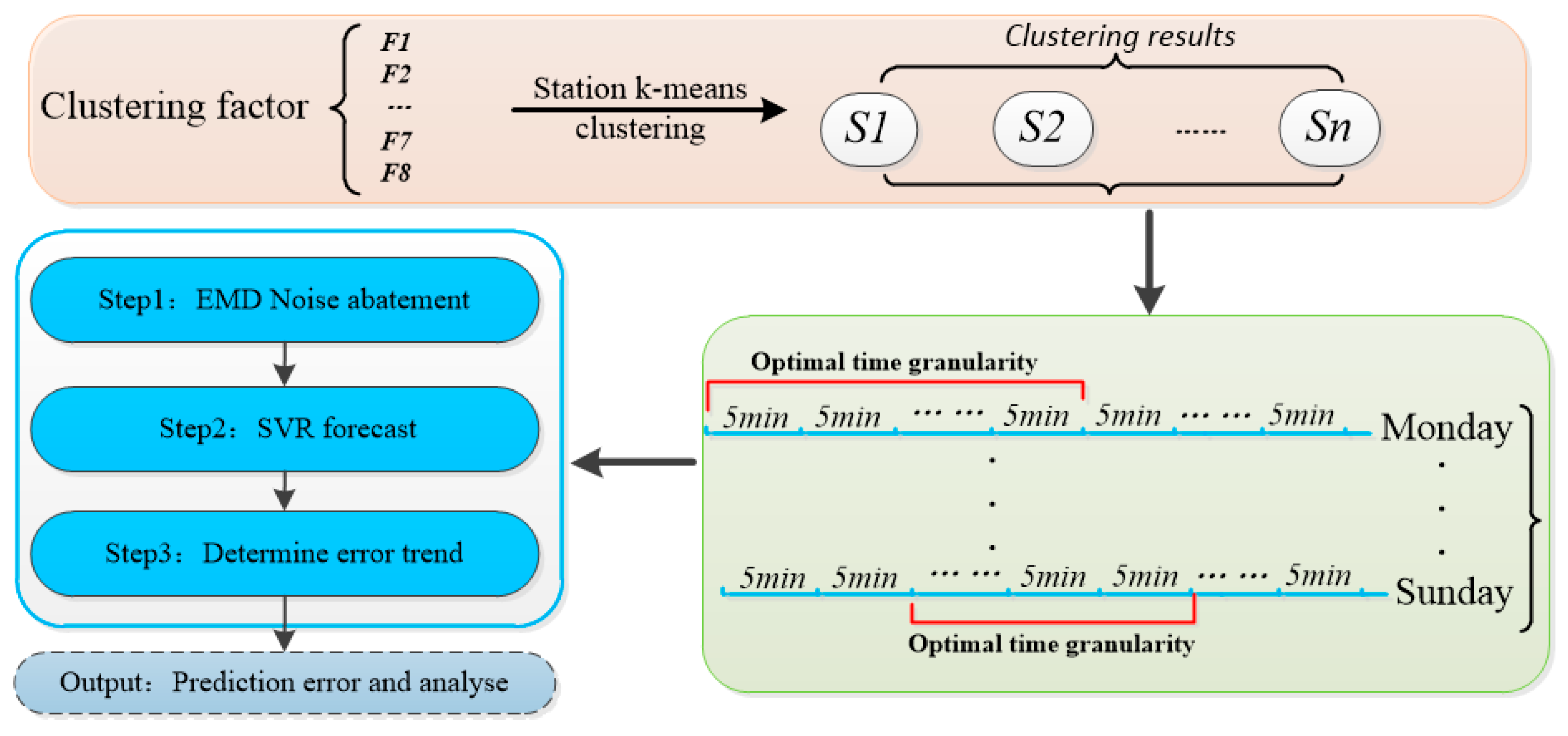
Figure 1. The overall framework of time granularity selection and passenger flow prediction.
Sustainability 11 05281 g001
Figure 2. Spatial presentation of different types of sites.
Sustainability 11 05281 g002
Figure 3. Passenger flow sharing rate. The y-axis means entrance passenger flow burden rate.
Sustainability 11 05281 g003
Figure 4. Pearson correlation coefficient under different time granularity of weekday’s morning and evening peaks.
Sustainability 11 05281 g004
Figure 5. Pearson correlation coefficient under different time granularity of weekend’s morning and evening peaks
Sustainability 11 05281 g005
Figure 6. Schematic diagram of time range selection data preprocessing.
Sustainability 11 05281 g006
Figure 7. Selection of four kinds of Station time periods by Pearson coefficient, Where, four points in the circle represent the maximum correlation coefficient of the passenger flow data of the station.
Sustainability 11 05281 g007
Figure 8. Schematic diagram of noise reduction of original data.
Sustainability 11 05281 g008
Figure 9. Prediction results of four stations by EMD-SVR Model.
Sustainability 11 05281 g009
Figure 10. Error rate and LBV fitting effect.
Sustainability 11 05281 g010
Table 1. Weight of clustering factors for different types of stations.
Station CategoryNumberF1F2F3F4F5F6F7F8
I type50.1100.6500.8790.1090.4000.4211.9241.89
II type500.1740.1040.1000.1380.3780.3411.0491.07
III type140.1110.0900.1010.1140.3940.3871.1351.330
IV type180.1110.1610.1340.0970.3870.3700.8550.930
Table 2. Characteristics of each station cluster.
Station (Number)ClusterStation (Number)ClusterStation (Number)Cluster
ClassDistanceClassDistanceClassDistance
HWZ(#1)III0.093SQ(#2)I0.078ZH(#3)I0.124
ZY(#4)I0.095HCL(#5)I0.179KYM(#6)I0.128
LDL(#7)I0.110YXM(#8)IV0.084SJQ(#9)I0.115
WLK(#10)III0.154CYM(#11)I0.187KFL(#12)IV0.288
THM(#13)I0.168WSL(#14)I0.088CLP(#15)I0.186
CH(#16)I0.183BP(#17)III0.172FZC(#18)I0.185
BKZ(#19)III0.175BY(#20)I0.134YDGY(#21)III0.148
XZZX(#22)I0.095FCWL(#23)I0.125STSG(#24)I0.090
DMGX(#25)I0.163LSY(#26)I0.141AYM(#27)I0.056
BDJ(#28)I0.181ZL(#29)III0.045YNM(#30)IV0.152
NSM(#31)IV0.084TYC(#32)I0.169XZ(#33)III0.403
WYJ(#34)I0.062HZZX(#35)I0.076SY(#36)III0.193
FXY(#37)I0.183HTC(#38)III0.137WQN(#39)II0.099
YHZ(#40)I0.148ZBBL(#41)I0.232YPM(#42)IV0.240
KJL(#43)IV0.269TBNL(#44)IV0.150JXC(#45)IV0.116
DYT(#46)III0.309BCT(#47)IV0.212QLS(#48)I0.080
YXM(#49)I0.098XNL(#50)III0.086CLGY(#51)I0.101
HJM(#52)I0.201SJJ(#53)I0.137XJM(#54)I0.147
GTM(#55)I0.159THT(#56)I0.123CBZX(#57)IV0.100
XHW(#58)II0.274WZ(#59)II0.237GJGW(#60)III0.218
SZ(#61)I0.094XZ(#62)II0.308BSQ(#63)III0.214
HTXC(#64)IV0.207HTDL(#65)IV0.110SZDD(#66)IV0.312
DCAJ(#67)I0.145FTL(#68)I0.127HTDD(#69)II0.122
JHT(#70)I0.115QJCX(#71)I0.112DTFR(#72)III0.213
XAKJ(#73)I0.279JZKJ(#74)I0.168HPM(#75)I0.121
DCS(#76)IV0.091HYD(#77)III0.118DMG(#78)IV0.150
DMGB(#79)I0.085YJZ(#80)I0.106BHC(#81)I0.111
CQL(#82)I0.167SZYY(#83)IV0.133WJL(#84)I0.152
FCJL(#85)I0.136FCSE(#86)IV0.174YSL(#87)IV0.133
Table 3. Prediction results of ARIMA Model at different stations.
StationTimeForecast ErrorRMSEStationTimeForecast ErrorRMSE
WQN
(I Type)
07:00–07:155.18%56.1STSG
(II Type)
07:00–07:156.42%41.2
07:15–07:305.72%42.107:15–07:307.66%32.7
07:30–07:454.71%61.207:30–07:457.33%33.4
07:45–08:003.41%41.707:45–08:006.23%27.6
08:00–08:154.24%44.908:00–08:156.44%22.3
08:15–08:306.22%53.408:15–08:306.72%32.9
08:30–08:454.32%42.308:30–08:457.23%28.5
08:45–09:004.82%34.108:45–09:007.14%22.7
ZL
(III Type)
07:00–07:158.22%45.4YXM
(IV Type)
07:00–07:156.43%44.2
07:15–07:307.12%35.207:15–07:306.22%37.2
07:30–07:458.22%44.207:30–07:455.72%31.4
07:45–08:007.41%36.207:45–08:005.33%34.1
08:00–08:157.31%34.408:00–08:155.43%30.3
08:15–08:307.65%36.208:15–08:306.14%28.3
08:30–08:458.11%33.208:30–08:456.53%22.1
08:45–09:007.54%37.408:45–09:005.44%27.4
Table 4. Performance criteria values of four model for prediction of passenger flow under optimal time selection
StationErrorEMD-SVRSVRARIMABPNNStationErrorEMD-SVRSVRARIMABPNN
WQNMAE29.438.733.856.4STSGMAE13.124.415.728.9
λ (%)3.164.533.414.42λ (%)5.668.436.238.87
RMSE46.462.552.482.7RMSE22.135.422.340.2
ZLMAE22.533.221.738.6YXMMAE17.226.619.327.2
λ (%)6.129.237.318.22λ (%)4.887.335.336.87
RMSE32.248.334.457.3RMSE27.241.130.345.1