The Effects of Energy Consumption, Economic Growth and Financial Development on CO₂ Emissions in China: A VECM Approach

Abstract

As one of the largest energy consumers and the greatest emitter of CO₂ in the world, China now confronts the dual challenge of reducing energy use while continuing to foster economic growth. To overcome this issue, there is a need of comprehensive economic, financial, and energy policy reforms to promote sustainable development. The objective of this paper is to examine the effects of economic growth, financial development and energy consumption on carbon dioxide emission (CO₂) in China from 1982 to 2017. The study applies Johansen cointegration test and vector error correction model (VECM) to investigate the long-term equilibrium and short-term causality relationship among the four variables. The causality is also checked by using the innovative accounting approach (IAA). The empirical results show the long-term cointegration relationship between them. Evidence shows that a unidirectional Granger causality running from energy consumption to financial development. Financial development and energy consumption have a statistically significant positive impact on CO₂ emissions. In the long run, economic growth can curb CO₂ emissions. Hence, financial innovation should be encouraged in the country to meet the demand of sustainable development. Nevertheless, optimizing energy structure and increasing the efficiency of energy utilization can never be left out from the process of development. We add light to policy makers with the construction of carbon trading to effectively address greenhouse effects in China.

1. Introduction

With the development of global economy, environmental pollution is becoming more and more serious [1,2,3,4,5,6]. Especially, the greenhouse effect caused by carbon dioxide (CO₂) has become one of the most concerned environmental problems in the world. This greenhouse effect has become an extremely serious threat to human survival and socio-economic sustainable development. Globally supplied energy is still growing to support the global economy, but the world is also facing the challenge of reducing greenhouse gas emissions. According to the International Energy Agency (IEA), global energy consumption increased by 2.3% year-on-year in 2018 due to strong global economic growth, almost double the average growth rate since 2010. Global natural gas consumption was 3.86 trillion cubic meters, up 5.3% year-on-year, 2.3 times the average growth rate of the past five years. Energy efficiency improvements are weak, and energy-related CO₂ emissions are hitting new highs. The sum of energy demand growth in China, the United States and India accounts for about 70% of the global total. It is predicted that by 2030, the world’s energy demand will increase by about 60% compared with 2000, and the growth of energy demand in developing countries will make it account for the majority of the increase in CO₂ emissions. According to analysis, developing countries will account for about 85% of the increase in CO₂ emissions from 2000 to 2030 [7]. Promoting greenhouse gas emission reduction is still an important task for human beings to cope with climate warming and promote sustainable use of resources. Whether it is the International Climate Convention negotiations; initiated in 1990, or the Kyoto Protocol (2005), the Bali Roadmap (2007), the Copenhagen Accord (2009) and Paris Agreement (2015), are committed to inhibit global warming through global cooperation.

To achieve sustainable development, we must consider the relationship between economic activities and environmental quality. There is substantial research on the relationship between economic growth, energy consumption, and carbon dioxide emissions. There are three research directions: the first part focuses on the relationship between economic growth and energy consumption; the second part focuses on the relationship between economic growth and carbon dioxide emissions; the third part puts the three variables under the same framework to study its dynamic causality. However, although many scholars have conducted a lot of research in the past 30 years, the relationship between the three has not been consistently concluded. The existing literature reveals that empirical studies differ substantially, for example, some studies investigate single countries [8,9,10] and others examine multiple countries [11,12,13,14]. With the introduction of additional variables, the relationship between the three has undergone new changes, such as urbanization [15], trade openness [16], foreign direct investment [17], industrialization [18]. In this regard, it is believed that additional variables can help explain the complexity surrounding the relationship between economic activity and the environment [19]. In recent years, financial development variables have attracted great attention from scholars. More and more scholars have begun to study financial development into the framework of economic growth, energy consumption and carbon dioxide emissions.

The choice of China is also motivated by the fact that China has been the second largest energy consumer and one of the fastest growing economies in the world. China is currently in the middle and late stages of industrialization, and has taken energy-saving and carbon-reduction measures to achieve a low-carbon economy. According to the China Statistical Yearbook 2018, from 2005 to 2017, the carbon dioxide intensity of GDP has dropped by 45%, and the annual average rate of decline has reached 4.9%. However, the Paris Agreement the proposed National Independent Contribution (NDC) targets, which is by 2030, the carbon dioxide intensity per unit of GDP will fall by 60% to 65% compared to 2005, and the proportion of non-fossil energy in primary energy consumption will increase to around 20%. Furthermore, China has experienced a significant rise in energy consumption and carbon emissions in recent decades. According to the World Energy China Outlook (2013–2014) forecast, the total energy demand in China will account for 24% of the world’s total energy demand in 2035, and the increase in energy demand will be as much as 38.5%. By then, the energy position of China will become more prominent in the world’s energy supply and demand pattern. Along with the rapid growth of the social economy, energy consumption continues to increase, and environmental pollutant emissions are further expanded, which has led to a severe test of carbon dioxide and sustainable economic development. At the same time, China’s financial development has grown rapidly in the past four decades, and its scale has expanded very rapidly. It has become an important world financial power. Therefore, we choose China as the research object to study the interaction between energy consumption, financial development, carbon dioxide emissions and economic growth, which has important policy significance for China to reduce carbon dioxide emissions.

The rest of this article is organized as follows. Section 2 briefly reviews the literature. Section 3 explains the data and methods. Section 4 discusses the empirical results. Section 5 summarizes the paper and discusses the policy implications.

2. Literature Review

The first strand of existing literature coops with a wide range of mixed result studies about energy consumption and economic growth. The Kraft and Kraft [20] investigated the causal relationship between these two variables in 1978. Through a study for the United States, covering the period between 1947 and 1974, they found that there is a one-way causal relationship between GNP and energy consumption. However, Akarca and Long [21] used data from 1947 to 1972 to conclude that there is no causal relationship between GNP and energy consumption. This also indicates that the choice of sample interval may affect the empirical results. Eden and Been [22] conclude that there is also no causal relationship between the two in USA from 1947 to 1979. Masih [23] studied the relationship between energy consumption and economic growth in six Asian countries based on Johansen cointegration test and VECM Granger test. The study found that only India, Pakistan and Indonesia have a long-term co-integration relationship between energy consumption and economic growth. Hye and Riaz [24] studied the causal relationship between energy consumption and economic growth in Pakistan from 1971 to 2007 by autoregressive distributed lag (ARDL) and Granger causality test. The study found that a two-ways causal relationship between energy use and economic growth in the Short term, while the long-run causality result shows that a one-way causal relationship exist runs from economic growth to energy use. Odhiambo [25] examined the relationship between energy consumption and economic growth in Tanzania, which shows the existence of one-way causality that runs from energy use to growth of the economy. Lin [26] used the Johansen–Juselius (JJ) cointegration test and VECM Granger causality test to prove that there is a long-term equilibrium relationship between China’s power consumption and economic growth. In recent years, some scholars have compared the relationship among regions. For example, Li [27] found that China’s energy consumption has a significant positive effect on economic growth and the eastern region of China has the most effective effect. Ahmed et al. [28] investigated the relationship between per capita electricity consumption and per capita real income, and the relationship between per capita energy consumption and economic growth in Pakistan, and found that there is a two-way causal relationship between them.

The second strand of existing literature on this topic provides empirical evidence on the relationship between economic growth and CO₂ emissions. Existing research on the relationship between carbon emissions and economic growth mainly includes linear relationships [29,30], N-curve relationships [31], and inverted U-shaped Curve relationships [32]. Although most scholars support Inverted U-curve relationship relationship [33,34,35], namely the environmental Kuznets curve (EKC), the findings of Robalino-López et al. [36] and Baek [37] showed that the inverted U-shaped curve does not hold, while Moomaw and Unruh [38], Martinez Zarzoso, and Bengochea-Morancho [39] found that there is an N-type relationship between economic growth and CO₂ emissions. The income per capita corresponding to the inflection point of the EKC curve varies widely, ranging from $13,260 to $80,000.Han and Lu [40] studied the Environmental Kuznets curve in different countries and the findings also vary greatly, showing the relationship of inverted U and linear. Some scholars [41,42] found that carbon dioxide emissions per capita increased monotonously with real income per capita, and there was no inflection point. However, Lantz and Feng [43] found that there was no significant relationship between per capita GDP and carbon dioxide emissions. There is no consensus on the relationship between carbon emissions and economic development [44]. Lin and Jiang [45] used the traditional environmental Kuznets model to simulate and predict the Kuznets curve of carbon dioxide in China on the basis of carbon dioxide emission prediction, and found that the results were quite different. The differences in the above literature conclusions are mainly due to the significant differences between the study region and the choice of empirical methods [46]. Henisz [47] pointed out that it is more reasonable to discuss the relationship between them from the perspective of causality compared with the EKC hypothesis. Since then, more and more scholars have chosen to use the causality test to explore the feedback mechanism of the interaction between economic growth and carbon dioxide emissions.

The third strand investigated the relationship between energy consumption, CO₂ emission and economic growth, beginning with Ang [48] who introduced the first study where he examined the connection among variables in France for 1960–2000 by co-integration analysis and error correction model (ECM).The outcome reveals that economic growth and carbon dioxide emissions have a U-shaped relationship in the long run, and that economic growth contributes to an increase in energy consumption, while the increase in energy consumption lead to an increase in carbon dioxide emissions. Soytas et al. [49] used co-integration methodology and VECM in Turkey and results indicate that a unidirectional causality exists from energy to GDP and energy consumption has a positive effect on economic growth. Tao and Song [50] measured the dynamic relationship between carbon dioxide emission, energy consumption, gross national income per capita and trade openness in China using the sample data of 1971–2008 in China. The results show that there is a long-term equilibrium relationship among them, and the long-term and short-term Granger causality exists at the same time. Arouri et al. [51] investigated the relationship between economic growth, energy consumption and carbon dioxide emissions in 12 countries of the Middle East and North Africa within the framework of panel unit root test and co-integration. The result is that there is a two-way causality between energy consumption and carbon dioxide in the long run. Govindaraju and Tang [52] applied the Granger causality approach in China and India, the result reveals the long-run relationship among the variables in China but no Indian. Cowan [53] studied the relationship between electricity consumption, economic growth and carbon dioxide emissions in BRICS from 1990 to 2010 under the framework of panel causality analysis. Osigwe and Arawomo [54] used the Granger causality approach to study the link between energy consumption, oil prices and economic growth in Nigeria. A two-way causal relationship between energy consumption and economic growth has been established. Asongu et al. [55] investigated the causal relationship between carbon dioxide emissions, energy consumption and GDP and there was a strong causal relationship between these variables.

In recent years, with the deepening of financial development, more and more scholars are paying attention to the relationship between financial development and economic growth [56,57]. In the modern economy, finance is the blood and accelerator of the economy, which affects the basic characteristics of energy consumption from many paths, and thus affects energy conservation and emission reduction. On the one hand, financial development will increase energy consumption. As the scale of financial development continues to expand and the efficiency of financial development continues to increase, consumers and businesses can obtain loans at a lower cost and in a more convenient way. For example, Sadorsky [58] studied the impact of financial development on energy consumption in 22 new economies from 1990 to 2006 based on the generalized method of moments(GMM). The empirical results show that when financial development is measured by stock market indicators, there is a significant positive relationship between financial development and energy consumption. Sadorsky [59] applied the same method to study nine economies along the east-central border of Europe, and found that when using bank indicators to measure financial development, the relationship between financial development and energy consumption was significantly positive. On the other hand, financial development will reduce energy consumption. Financial development encourages enterprises to introduce high-tech and equipment for energy conservation and environmental protection, and provide financial support for the development of knowledge-intensive and technology-intensive high-tech industries. Therefore, financial development can reduce energy consumption. For example, Tamazian and Chousa et al. [60] found that financial development and economic growth could have an impact on the environmental quality, which would contribute to the reduction of carbon dioxide emissions and play a positive role in the improvement of environmental quality. Tamazian and Rao [61] studied the relationship between financial development and environmental pollution in 24 transition countries based on the generalized method of moments (GMM) to control endogeneity. They believe that foreign investment found to measure financial development helps reduce carbon dioxide emissions per capita. Moreover, in addition to incorporating financial development into economic growth, energy consumption and carbon dioxide research, researchers have also added variables such as foreign direct investment (FDI), trade openness, and urbanization. For example, Farhani and Ozturk [62] empirically examine the link relationship between CO₂ emissions, economic growth, energy consumption, financial development, trade openness, and urbanization in Tunisia for 1971–2012 by ARDL-ECM method. Moreover, they find that financial development has a positive and significant impact on environmental pollution. The monotonic positive relationship is also found between GDP and CO₂ emissions.

3. Empirical Analysis

3.1. Data

This study uses annual data of China covering the period 1982–2017.Carbon dioxide emission (CO₂) is expressed in kilo terms (k_t). Energy consumption (EN) is measured by total energy consumption per capita (kg of oil equivalent). Domestic credit to private sector as share of GDP is used as the proxy for financial development (FD). Economic growth (GDP) is measured as the percentage change of real GDP per capita. The data on CO₂ emission and financial development are downloaded from the World Bank’s World Development Indicators (World Development Indicators). The data on Economic growth and Energy consumption are extracted from China Statistical Yearbook. Figure 1 shows the trends in CO₂ emission, energy consumption, economic growth, and financial development. In order to avoid possible heteroscedasticity, all data are transformed to natural logarithm.

3.2. Modeling Framework

To investigate the long-term equilibrium and short-term dynamic relationship between carbon dioxide emissions and financial development, energy consumption and economic growth in China, this paper adopts Johansen cointegration test and vector error correction model (VECM). Since most time series are non-stationary, direct regression will lead to “pseudo-regression”. Therefore, Engle and Granger [63] proposed the concept of cointegration, which means the long-term stable relationship exists between economic variables. Sims and Watson [64] further studied and derived the analysis of multivariate models with unit root variables. Based on this, VECM model was formally proposed. The VECM model is widely used for exploring the long-term and short-term equilibrium relations with co-integration variables. If the variables are cointegrated in this study, the VECM equation is expressed as follows:

$$\begin{array}{c}{\mathsf{\Delta }\mathrm{LNGDP}}_t={\mathsf{\phi }}_1+{\sum }_{i=1}^n{\alpha }_{1i}\Delta LNGD{P}_{t-i}+{\sum }_{j=1}^n{\beta }_{1j}\Delta LNF{D}_{t-j}+{\sum }_{k=1}^n{\gamma }_{1k}\Delta LNE{N}_{t-k}\\ +{\sum }_{q=1}^n{\delta }_{1q}\Delta LNCO{2}_{t-q}+{\xi }_{1}EC{T}_{t-1}+{\mu }_{1t}\end{array}$$

(1)

$$\begin{array}{c}{\mathsf{\Delta }\mathrm{LNFD}}_t={\mathsf{\phi }}_2+{\sum }_{i=1}^n{\alpha }_{2i}\Delta LNF{D}_{t-i}+{\sum }_{j=1}^n{\beta }_{2j}\Delta LNGD{P}_{t-j}+{\sum }_{k=1}^n{\gamma }_{2k}\Delta LNE{N}_{t-k}\\ +{\sum }_{q=1}^n{\delta }_{2q}\Delta LNCO{2}_{t-q}+{\xi }_{2}EC{T}_{t-1}+{\mu }_{2t }\end{array}$$

(2)

$$\begin{array}{c}{\mathsf{\Delta }\mathrm{LNEN}}_t={\mathsf{\phi }}_3+{\sum }_{i=1}^n{\alpha }_{3i}\Delta LNE{N}_{t-i}+{\sum }_{j=1}^n{\beta }_{3j}\Delta LNGD{P}_{t-j}+{\sum }_{k=1}^n{\gamma }_{3k}\Delta LNF{D}_{t-k}\\ +{\sum }_{q=1}^n{\delta }_{3q}\Delta LNCO{2}_{t-q}+{\xi }_{3}EC{T}_{t-1}+{\mu }_{3t}\end{array}$$

(3)

$$\begin{array}{c}\mathsf{\Delta }\mathrm{LNCO}{2}_t={\mathsf{\phi }}_4+{\sum }_{i=1}^n{\alpha }_{4i}\Delta LNCO{2}_{t-i}+{\sum }_{j=1}^n{\beta }_{4j}\Delta LNGD{P}_{t-j}+{\sum }_{k=1}^n{\gamma }_{4k}\Delta LNF{D}_{t-k}\\ +{\sum }_{q=1}^n{\delta }_{4q}\Delta LNE{N}_{t-q}+{\xi }_{4}EC{T}_{t-1}+{\mu }_{4t}\end{array}$$

(4)

where $\mathsf{\phi }$, $\mathsf{\alpha }$,$\mathsf{\beta },\mathsf{\gamma }$, and $\mathsf{\delta }$ are coefficients of the polynomial; n is the optimal lag; ECT_t−1 is the correction term. Take Equation (1) as an example, it expresses the causality test model from LNFD, LNEN and LNCO2 to LNRGDP. If the null hypothesis (H0: ${\mathsf{\beta }}_{1\mathrm{j}}$ = ${\mathsf{\gamma }}_{1\mathrm{k}}$= ${\mathsf{\delta }}_{1\mathrm{q}}=$0) is rejected in Equation (1), there is a short-term Granger causality from LNFD, LNEN and LNCO2 to LNGDP. The coefficient ${\mathsf{\xi }}_1$ of the error correction term shows the speed of adjustment towards equilibrium. If the null hypothesis (H0: ${\mathsf{\xi }}_1$ = 0) is rejected, long term Granger causality is established from right to left.

In addition, we implement the IAA (Innovative Accounting Approach) that includes advanced generalized forecast error variance decomposition and generalized impulse response techniques [65]. It is argued in recent literature that Granger causality methods such as the VECM Granger causality test have some limitations. Causality test cannot capture the relative strength of causal relationships between variables beyond the selected time period, which weakens the reliability of the causal relationship results [66]. In addition, the VECM Granger method does not tell us the ratio of contributions [67]. To solve this problem, we apply the IAA to examine the effects of energy consumption, economic growth and financial development on CO₂ emissions. Pesaran and Shin [68] pointed out that unlike the traditional impulse response analysis, the generalized impulse responses does not require orthogonalization of shocks and is invariant to the ordering of the variables in the VAR. Furthermore, it fully takes account of the historical patterns of correlations observed amongst the different shocks. Subsequently, Pesaran and Shin [69] argued that the generalized forecast error variance decomposition method shows a proportional contribution in a variable due to the innovative shocks stemming in other variables. The main advantage of this method is that it is not sensitive to the ordering of variables and estimates the simultaneous shock affects. Therefore, this paper examines causality by using innovative accounting methods (IAA).

4. Empirical Results

4.1. Unit Root Analysis

Since the time series selected in this paper are all time series, in order to avoid a spurious regression phenomenon, it is necessary to conduct a unit root test for each variable before the analysis. This paper adopts the augmented Dickey-Fuller (ADF) and Phillips-Perron (PP) tests and the test results are shown in the

Table 1. Results of the unit root test.

Variables	Test Type	ADF	PP	1% Critical Value	5 %Critical Value	Result
LNFD	CT	−2.689063(0)	−2.589856(4)	−4.243644	−3.544284	Non-stationary
DLNFD	C	−5.429577(0)	−4.655730(1)	−3.639407	−2.951125	stationary
LNGDP	CT	−2.495055(1)	−1.929439(2)	−4.243644	−3.544284	Non-stationary
DLNGDP	C	3.460473(0)	−3.532214(1)	−3.639407	−2.951125	stationary
LNCO2	CT	−3.185076(1)	−1.794890(3)	−4.243644	−3.544284	Non-stationary
DLNCO2	C	−3.147978(0)	−2.55326(1)	−3.639407	−2.951125	stationary
LNEN	CT	−1.707846(1)	−1.889023(3)	−4.243644	−3.544284	Non-stationary
DLNEN	C	−3.848236(0)	−3.937483(3)	−3.639407	−2.951125	stationary

Note: The “D” used in front of the variables indicates the first difference; CT stands for constant and trend; C stands for constant. The parentheses of the ADF test value indicate the lag length, and the parentheses of the PP test value indicate the bandwidth.

.

It can be seen from the

Table 2. VAR Lag Order Selection Criteria.

Lag	LogL	LR	FPE	AIC	SC	HQ
0	64.92185	NA	2.93E−07	−3.692233	−3.510839	−3.631200
1	248.3995	311.3560	1.15E−11	−13.84240	−12.93542	−13.53723
2	278.3852	43.61560 *	5.19E−12 *	−14.69002 *	−13.05746 *	−14.14071 *
3	292.8496	17.53254	6.44E−12	−14.59695	−12.23881	−13.80351

Note: * indicates lag order selected by the criterion; LR: sequential modified LR test statistic (each test at 5% level); FPE: Final prediction error; AIC: Akaike information criterion; SC: Schwarz information criterion; HQ: Hannan-Quinn information criterion.

that that the ADF Value of LNFD is −2.689063 and PP test value is −2.589856, both of which were greater than the critical value of 0.05 significance levels. Therefore, the null hypothesis that there is a unit root should be accepted, indicating that LNFD is a non-stationary sequence. While DLNFD has the ADF and the PP inspection values that are less than the critical value of 0.05 significant levels, indicating the sequence is stable after a first difference. Similarly, The Table 2 shows that the LNGDP, LNCO₂ and LNEN are all non-stationary, and they are stationary in first differences. Thus, All the four variables are I(1).

4.2. Cointegration Test

After the unit root test, all the variables are all first-order differential stationary sequences, so there may be a co-integration relationship. To determine the cointegration of time series variables, this paper uses the Johansen cointegration test together with a Vector Autoregressive (VAR) analysis.

Before co-integration test, the optimal lag length can be comprehensively determined according to AIC, SC, LR, FPE and HQ. As seen from Table 2, the optimal lag length obtained in this paper is 1, and the specific results of the Johansen cointegration test are shown in the

Table 3. Results of the Johansen cointegration test.

Null Hypothesis	Trace Statistic	5% Critical Value	Prob. **	Max-Eigen Statistic	5%Critical Value	Prob. **
R = 0	53.64706 *	47.85613	0.0130	32.85503 *	27.58434	0.0095
R $\le 1$	20.79203	29.79707	0.3708	14.06902	21.13162	0.3594
R $\le 2$	6.723007	15.49471	0.6101	6.242698	14.26460	0.5823
R $\le 3$	0.480309	3.841466	0.4883	0.480309	3.841466	0.4883

Note: Trace test indicates 1 cointegrating eqn(s) at the 0.05 level; * denotes rejection of the hypothesis at the 0.05 level; ** MacKinnon-Haug-Michelis (1999) p-values; Max-eigenvalue test indicates 1 cointegrating eqn(s) at the 0.05 level; * denotes rejection of the hypothesis at the 0.05 level.

.

There are generally two methods for Johansen cointegration test, which are trace and maximal eigenvalue tests. The results of both methods are shown in Table 3, the null hypothesis that claims the absence of no co-integration, is rejected when the P value is less than 0.05 at the 5% significance level under both the trace statistic and the maximum eigenvalue method. Both tests fail to reject the null hypothesis (R ≤ 1) that a maximum of one cointegration exists at the 0.05 significance level, Therefore, there is a cointegration relationship between the financial development, energy consumption, economic growth and CO₂ emissions.

4.3. Causality Analysis Using a VECM

After determining the cointegration relationship between variables, a Granger causality test is conducted to formulate appropriate energy policies for sustainable economic growth. Since the variables are cointegrated, we used the vector error correction model (VECM) framework as described in the previous section to achieve the goal. Granger [70] pointed out that vector error correction method (VECM) is more appropriate to examine the causality between the series if the variables are integrated at I(1). Therefore, we apply the VECM Granger causality test by Engle and Granger [63] to investigate the direction of causality between financial development, economic growth, energy consumption and CO₂ emissions.

The parameters of the VECM model can be estimated as shown in the

Table 4. Vector Error Correction Estimates.

Error Correction	D(LNCO2)	D(LNGDP)	D(LNFD)	D(LNEN)
ECTt-1	−0.636131	−0.429491	0.101922	0.573628
	[−4.19226]	[−1.05848]	[0.28813	[4.16656]
D(LNCO2(−1))	1.438273	0.923703	−0.676341	0.038017
	[7.92506]	[1.90335]	[−1.59865]	[0.23088]
D(LNGDP(−1))	0.005526	0.283941	0.442957	−0.098721
	[0.06875]	[1.32100]	[2.36393]	[−1.35363]
D(LNFD(−1))	−0.076717	−0.283798	0.216823	−0.073455
	[−0.90923]	[−1.25782]	[1.10234]	[−0.95951]
D(LNEN(−1))	0.072475	0.350433	−0.238277	−0.010714
	[0.63188]	[1.14255]	[−0.89116]	[−0.10296]
C	−0.025339	0.024400	0.019459	0.060954
	[−1.44010]	[0.51857]	[0.47441]	[3.81809]
R-squared	0.734460	0.378264	0.293456	0.762613
Adj. R-squared	0.687043	0.267240	0.167288	0.720222
F-statistic	15.48913	3.407037	2.325910	17.99017

Note: t-statistics are provided in square brackets.

According to the test results of the VECM in Table 4, we find that ECT _t−1 are negative and statistically significant at the 5% significance level for Equations (4). In addition, the significant of ECT_t-1 also exhibiting that if the system expose to shock it will convergence to the long-run equilibrium at a relatively slow speed for LNCO2(−0.6361). Next, we perform the Granger causality test to check the causality relationships among the variables from the application of VECM. The direction of causality can be divided into short-term and long-term causal relationships and the results are shown in the

Table 5. Results of the vector error correction model (VECM) Granger causality test.

Variable	Type of Granger Causality					Conclusion
	Short Run				Long Run
	DLNCO2	DLNEN	DLNFD	DLNGDP	ECTt-1
DLNCO2		28.9138 ***	2.95443 *	4.9633 **	−0.6361 ***	CO2 > EN;CO2 > FD;
		[0.0000]	[0.0956]	[0.0333]	[−4.1923]	CO2 > GDP
DLNEN	0.87589		0.8662	1.72607	0.5736***	EN $\ne$> CO2; EN $\ne$> FD
	[0.3566]		[0.3592]	[0.2226]	[4.1666]	EN $\ne$> GDP
DLNFD	0.5160	7.04230 **		1.5492	0.1019	FD $\ne$> CO2; FD > EN
	[0.4779]	[0.0124]		[0.2226]	[0.2881]	FD $\ne$> GDP
DLNGDP	3.8873 *	5.9769 **	3.6110 *		−0.4295	GDP > CO2; GDP > EN;
	[0.0576]	[0.0204]	[0.0667]		[−1.0585]	GDP > FD

Note: In the short-term causality test, the F-statistic value is used, and the value of the square brackets is the corresponding p-value; In the long-term causality test, t-statistics are provided in square brackets; *, **, *** denote significance at the 10%, 5%, and 1% levels, respectively; > means that the left side can cause the right side; $\ne$> means that the left side cannot cause the right side;.

.

From the short-term causality test, CO₂ emissions are the cause of energy consumption and economic growth at a significant level of 0.05. At a significant level of 0.1, CO₂ emissions are the Granger cause of financial development, indicating CO₂ carbon emissions have a certain predictive effect on energy consumption, financial development and economic growth in the short term. Energy consumption is not the Granger cause of CO₂ emissions, financial development and economic growth at a significant level of 0.05. Economic growth is the Granger cause of energy consumption at the level of significance of 0.05, and economic growth is also the Granger cause of CO₂ emissions and financial development at the level of significance of 0.1.

Results in Table 5 show that there is a unidirectional Granger causality running from energy consumption to financial development at the 5% significant level in China. That is, an increase in financial development will bring about an increase in energy consumption, but not vice versa. This effect can be explained as: on the one hand, the continuous inflow of consumer credit to the private sector has injected more vitality into our economic system, stimulating the purchase and use of high-energy consumer goods such as automobiles, air conditioners, and houses. This has increased the consumption of energy; on the other hand, the scale of the private sector credit business has been increasing, providing more and more convenient financial support for the development of private enterprises, helping private enterprises to further expand production, thereby increasing the demand for energy.

The long-term causality test shows that the bidirectional causality relationship only exists between CO₂ emissions and energy consumption. This finding is consistent with existing energy literature such as Hatzigeorgiou et al. [71] and later on with Shahbaz et al. [66]. This consensus provides policy makers to further validate the direction of causality between CO₂ emissions and energy consumption in China for future energy planning. This means that in the current setting, it is difficult for the Chinese economy to find carbon emissions from decarbonization, and there is a need of energy structure adjustment policies.

4.4. Impulse Response Function Analysis

In order to investigate the effect of innovations in all variables in the system on CO₂ emissions, the impulse response analysis is conducted. The impulse responses of CO₂ emissions to one standard deviation innovations to energy consumption, financial development, and economic growth are displayed in Figure 2, and the results of generalized pulse function response of LNCO2 are shown in the Appendix A

Table A1. Results of Generalized pulse function Response of LNCO2.

Period	LNCO2	LNGDP	LNFD	LNEN
1	0.025461	0.004303	−0.000999	0.005157
2	0.049171	0.002156	0.002683	0.025585
3	0.062756	−0.004616	0.008579	0.046366
4	0.064874	−0.013061	0.015029	0.059907
5	0.058570	−0.019489	0.019645	0.063673
6	0.048792	−0.022073	0.021254	0.059584
7	0.040059	−0.021067	0.020168	0.051659
8	0.035056	−0.017991	0.017619	0.043907
9	0.034312	−0.014607	0.014980	0.038960
10	0.036708	−0.012200	0.013208	0.037624
11	0.040397	−0.011291	0.012640	0.039192
12	0.043681	−0.011709	0.013083	0.042183
13	0.045551	−0.012878	0.014056	0.045097
14	0.045814	−0.014150	0.015048	0.046948
15	0.044898	−0.015049	0.015710	0.047437
16	0.043503	−0.015385	0.015918	0.046834
17	0.042267	−0.015222	0.015746	0.045702
18	0.041569	−0.014779	0.015378	0.044604
19	0.041477	−0.014299	0.015004	0.043911
20	0.041827	−0.013962	0.014756	0.043733
21	0.042355	−0.013838	0.014680	0.043965
22	0.042819	−0.013902	0.014746	0.044394
23	0.043080	−0.014070	0.014886	0.044807
24	0.043112	−0.014251	0.015027	0.045066
25	0.042978	−0.014377	0.015119	0.045131
26	0.042779	−0.014423	0.015147	0.045042
27	0.042604	−0.014398	0.015122	0.044880
28	0.042507	−0.014334	0.015069	0.044724
29	0.042496	−0.014266	0.015016	0.044627
30	0.042547	−0.014219	0.014981	0.044603
31	0.042622	−0.014202	0.014971	0.044638
32	0.042688	−0.014211	0.014981	0.044699
33	0.042724	−0.014236	0.015001	0.044758
34	0.042728	−0.014261	0.015021	0.044794
35	0.042708	−0.014279	0.015034	0.044803
36	0.042680	−0.014285	0.015038	0.044789

. In the Figure, the horizontal axis represents the number of impulse response periods, the vertical axis represents the response intensity, and the solid line is the impulse response curve.

The Figure 2a shows the positive response in carbon emissions due to standard shocks stemming in energy consumption. When one standard error shock in energy consumption affects CO₂ emission, the effect is positive and follows a decreasing trend. In phase 5, the maximum response is reached, the response intensity is 0.064, and then the fluctuation is declining. The 10th period reaches the minimum effect for the first time and the value was 0.038, followed by a trend of rising volatility. The second period reached the highest point in the 15th period, and the response value was 0.047. Then, the trend of volatility decreased, and the 25th period began to converge. The impulse response function indicates that the positive impact of energy consumption has a significant positive impact on CO₂ emissions, and the promotion effect is the strongest in the short term, and the impact of energy consumption on CO₂ emissions has certain sustainability. Their effects seem to support each other and hence environmental degradation.

The Figure 2b shows the impulse responses of CO₂ emissions to one standard deviation innovations to financial development. The response in CO₂ emissions is positive by shocks stemming in financial development, which indicates that the financial development has a significant positive impact on CO₂ emissions. This result is in line with the finding of Sariannidis et al. [72]. Combined with the results of the Granger causality test, the implication of these findings is that the financial development at present has not yet fully developed to the extent that it can bring about sustainable economic growth; therefore, it is necessary to further deepen finance to promote financial development to the level where it can reduce carbon dioxide emissions, mitigate global warming, and improve environmental quality.

As shown in Figure 2c, the response of CO₂ emissions to a shock on economic growth appears positive in the first 2 periods and then turns to be negative and exhibits a downward trend. This finding seems to support Ohlan [73] and Mallick et al. [74] finding of the presence of EKC. The impulse response function indicates that there is a certain lag in the impact of economic growth on CO₂ emissions. In the long run, economic growth has a significant and sustained inhibition of CO₂ emissions, indicating that economic growth can inhibit CO₂ emissions in the long term.

4.5. Variance Decomposition Analysis

In order to compare the contribution extent of the percentage of financial development, energy consumption and economic growth to the change in CO₂ emissions, the variance decomposition approach is used in the paper. The results of variance decomposition of specific variables are shown in the

Table 6. Results of the variance decomposition of CO₂ emissions.

Period	S.E.	LNCO2	LNGDP	LNFD	LNEN
1	0.025461	100.0000	0.000000	0.000000	0.000000
2	0.057699	92.09613	1.171115	0.001806	6.730951
3	0.092207	82.38396	3.264394	0.000790	14.35085
4	0.123097	73.99907	5.752938	0.001224	20.24677
5	0.147202	67.57938	8.125985	0.006005	24.28863
6	0.164226	63.12225	10.03725	0.017450	26.82305
7	0.175695	60.34875	11.35381	0.033294	28.26414
8	0.183723	58.83062	12.12755	0.048675	28.99315
9	0.190201	58.14582	12.50037	0.059873	29.29394
10	0.196496	57.97019	12.61539	0.065979	29.34844
11	0.203393	58.05031	12.59125	0.068109	29.29033
12	0.211107	58.16675	12.52976	0.067996	29.23550
13	0.219392	58.16710	12.50678	0.067157	29.25896
14	0.227780	58.00736	12.55358	0.066626	29.37244
15	0.235841	57.73376	12.65849	0.066889	29.54086

.

From Table 6, it is indicated that as time goes by, the contribution extent of CO₂ emissions itself to the change in CO₂ emissions has a downward trend, while those of financial development, energy consumption and economic growth rise steadily. In addition, in spite of the contribution extent of CO₂ emissions itself, energy consumption has the greatest impact on carbon emissions, and its contribution level is increasing by nearly 30%. This result is in line with the finding of Ohlan [73] in the context of India. The influence of economic growth also shows a steadily rising trend whose contribution reaches to 12%, while the role of financial development in explaining variation in change in carbon emission is negligible. Therefore, we can say, that China’s energy consumption should be the most crucial factor affecting CO₂ emissions in the next decade or so, which further validates the importance of low-carbon economic pattern in China. Overall, this suggests that efforts to increase renewable energy production are more important than actions that directly reduce carbon emissions.

5. Conclusions and Policy Recommendation

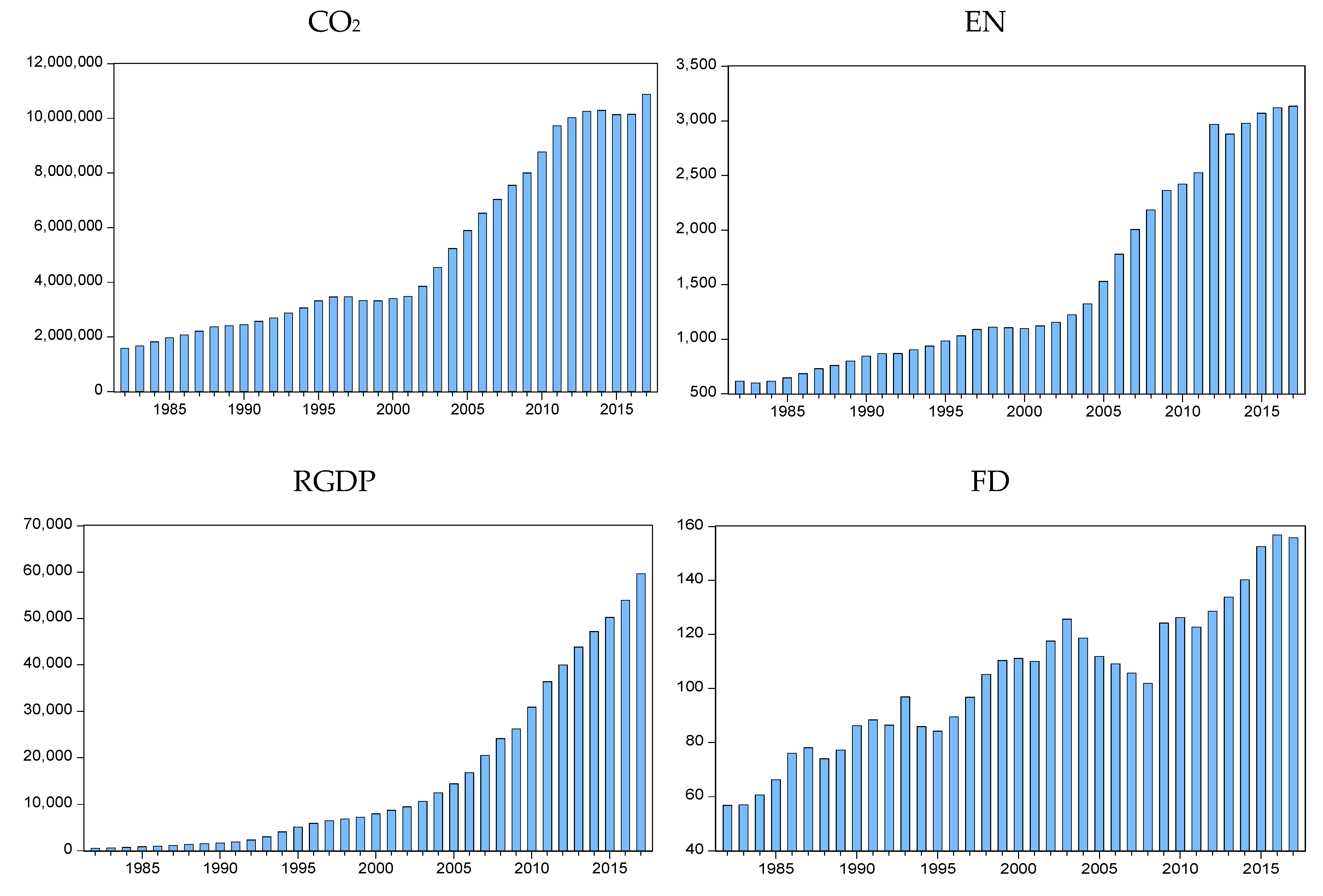
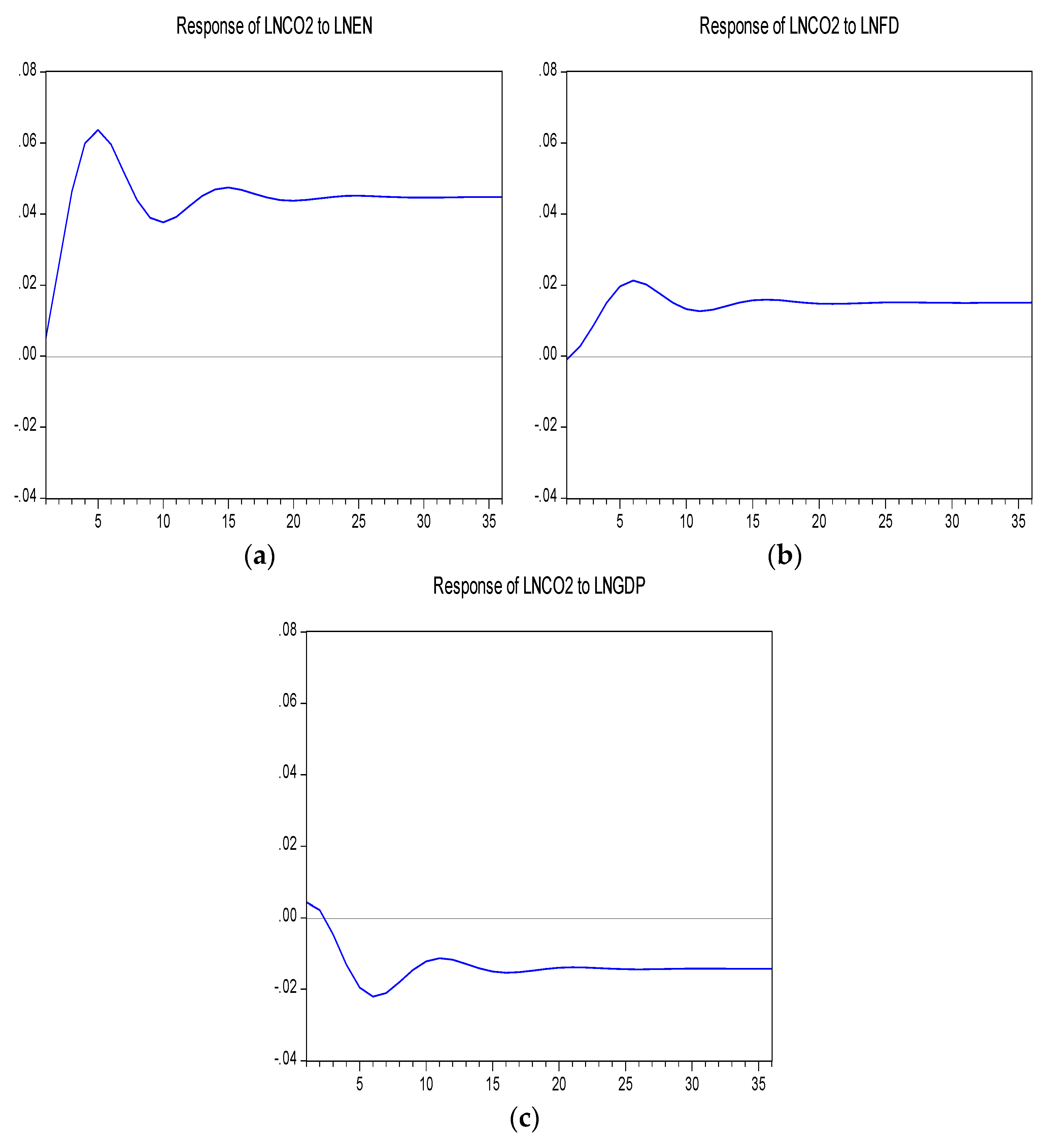
This paper investigates the effects of energy consumption, economic growth and financial development on CO₂ emissions in China over the period of 1982–2017. The empirical results show that there is a long-term cointegration relationship between the four variables. According to the Granger causality test, in the short run, carbon dioxide emissions have a positive effect on energy consumption, economic growth and financial development; economic growth and financial development are Granger reasons for energy consumption. In the impulse response test results, it can be seen that there is a positive two-way causal relationship between CO₂ emissions and energy consumption; financial development will promote carbon dioxide emissions in the short term, while the increase of CO₂ emissions will inhibit financial development. Economic growth can inhibit CO₂ emissions in the long run, and carbon dioxide emissions are more stimulating in the short term. From the results of variance decomposition, it can be seen that the variance contribution of CO₂ emission prediction error is mainly from energy consumption and economic growth.

These results have some policy implications for China. First, we should steadily promote financial innovation, low-carbon finance, and green credit business. It is necessary to improve the development level of the stock market, strengthen the supervision and guidance of the capital market system, improve the information disclosure and other related systems in the capital market, and actively play the role of the stock market in promoting green energy conservation. Second, Energy consumption in China is exacerbating carbon dioxide emissions when energy consumption structure is still dominated by high-carbon energy such as coal. Therefore, the government should optimize energy structure, increase the efficiency of energy utilization and realize energy sustainable development in China. There must be a clear and specific strategy for encouraging renewable energy, such as providing adequate policy support in technological innovation. China has promoted the consumption revolution, strengthened energy technology innovation and energy system reform, and strived to build a clean, low-carbon, safe and efficient energy system, and accelerated the process of low-carbonization of energy. From 2005 to 2017, the proportion of non-fossil energy in primary energy consumption was increased to 13.8%, the proportion of natural gas was increased to 7.0%, the corresponding proportion of coal was dropped to 60.4%. Third, in view of the characteristics of China’s energy consumption, carbon emissions, financial development and economic growth, market-based measures can be adopted to improve environmental governance. Ren et al. [75] found that carbon trading policy is helpful to improve energy structure and reduce CO₂ emissions by investigating China’s 30 provincial-level administrative regions in 2008–2015 panel data. Therefore, the government should continue to promote the construction of China’s carbon market, improve the participation of enterprises through reasonable pricing and quota allocation, and at the same time cooperate with other environmental protection policies to jointly promote sustainable development.

References

1. Guo, J.Y.; Zhou, Y.L. Transformation of heavy metals and dewaterability of waste activated sludge during the conditioning by Fe2+-activated peroxymonosulfate oxidation combined with rice straw biochar as skeleton builder. Chemosphere 2019. [Google Scholar] [CrossRef]
2. Li, F.; Qiu, Z.Z.; Zhang, J.D.; Liu, C.Y.; Cai, Y.; Xiao, M.S.; Zhu, L.Y. Temporal variation of major nutrients andprobabilistic eutrophication evaluation based on stochastic-fuzzy method in Honghu Lake, Middle China. Sci. China Technol. Sci. 2019, 62, 417–426. [Google Scholar] [CrossRef]
3. Zeng, J.J.; Liu, T.; Feiock, R.; Li, F. The impacts of China’s provincial energy policies on major air pollutants: A spatial econometric analysis. Energy Policy 2019, 132, 392–403. [Google Scholar] [CrossRef]
4. Guo, J.Y.; Jiang, S.L.; Pang, Y.J. Rice straw biochar modified by aluminum chloride enhances the dewatering of the sludge from municipal sewage treatment plant. Sci. Total Environ. 2019, 654, 338–344. [Google Scholar] [CrossRef]
5. Li, F.; Zhang, J.D.; Liu, W.; Liu, J.; Huang, J.; Zeng, G. An exploration of an integrated stochastic-fuzzypollution assessment for heavy metals in urban topsoil based on metal enrichment and bioaccessibility. Sci. Total Environ. 2018, 644, 649–660. [Google Scholar] [CrossRef]
6. Guo, J.Y.; Chen, C.; Jiang, S.L.; Zhou, Y.L. Feasibility and mechanism of combined conditioning with coagulant and flocculant to enhance sludge dewatering. ACS Sustain. Chem. Eng. 2018, 6, 10758–10765. [Google Scholar] [CrossRef]
7. World Energy Outlook. Available online: https://www.oecd-ilibrary.org/energy/world-energy-outlook_20725302 (accessed on 6 August 2019).
8. Akbostancı, E.; Türüt-Aşık, S.; Tunç, G.İ. The relationship between income and environment in Turkey: Is there an environmental Kuznets curve? Energy Policy 2009, 37, 861–867. [Google Scholar] [CrossRef]
9. Fodha, M.; Zaghdoud, O. Economic growth and pollutant emissions in Tunisia: An empirical analysis of the environmental Kuznets curve. Energy Policy 2010, 38, 1150–1156. [Google Scholar] [CrossRef]
10. Ghosh, S.; Kanjilal, K. Long-term equilibrium relationship between urbanization, energy consumption and economic activity: Empirical evidence from India. Energy 2014, 66, 324–331. [Google Scholar] [CrossRef]
11. Yu, E.S.H.; Choi, J.-Y. The causal relationship between energy and GNP: An international comparison. J. Energy Dev. 1985, 10, 249–272. [Google Scholar]
12. Al-Iriani, M.A. Energy–GDP relationship revisited: An example from GCC countries using panel causality. Energy Policy 2006, 34, 3342–3350. [Google Scholar] [CrossRef]
13. Ozcan, B. The nexus between carbon emissions, energy consumption and economic growth in Middle East countries: A panel data analysis. Energy Policy 2013, 62, 1138–1147. [Google Scholar] [CrossRef]
14. Bekhet, H.A.; Matar, A.; Yasmin, T. CO2 emissions, energy consumption, economic growth, and financial development in GCC countries: Dynamic simultaneous equation models. Renew. Sustain. Energy Rev. 2017, 70, 117–132. [Google Scholar] [CrossRef]
15. Shahbaz, M.; Lean, H.H. Does financial development increase energy consumption? The role of industrialization and urbanization in Tunisia. Energy Policy 2012, 40, 473–479. [Google Scholar] [CrossRef] [Green Version]
16. Halicioglu, F. Residential electricity demand dynamics in Turkey. Energy Econ. 2007, 29, 199–210. [Google Scholar] [CrossRef]
17. Ibrahiem, D.M. Renewable Electricity Consumption, Foreign Direct Investment and Economic Growth in Egypt: An ARDL Approach. Procedia Econ. Financ. 2015, 30, 313–323. [Google Scholar] [CrossRef] [Green Version]
18. Liu, X.; Bae, J. Urbanization and industrialization impact of CO2 emissions in China. J. Clean. Prod. 2018, 172, 178–186. [Google Scholar] [CrossRef]
19. Shahbaz, M.; Solarin, S.A.; Mahmood, H.; Arouri, M. Does financial development reduce CO2 emissions in Malaysian economy? A time series analysis. Econ. Model. 2013, 35, 145–152. [Google Scholar] [CrossRef]
20. Kraft, J.; Kraft, A. On the Relationship between Energy and GNP. J. Energy Dev. 1978, 3, 401–403. [Google Scholar]
21. Akarca, A.T.; Long, T.V. On the Relationship between Energy and GNP: A Reexamination. J. Energy Dev. 1980, 5, 326–331. [Google Scholar]
22. Yu, E.S.H.; Hwang, B.-K. The relationship between energy and GNP: Further results. Energy Econ. 1984, 6, 186–190. [Google Scholar] [CrossRef]
23. Masih, A.M.M.; Masih, R. Energy consumption, real income and temporal causality: Results from a multi-country study based on cointegration and error-correction modelling techniques. Energy Econ. 1996, 18, 165–183. [Google Scholar] [CrossRef]
24. Hye, Q.M.A.; Riaz, S. Causality between Energy Consumption and Economic Growth: The Case of Pakistan. Lahore J. Econ. 2008, 13, 45–58. [Google Scholar]
25. Odhiambo, N.M. Energy consumption and economic growth nexus in Tanzania: An ARDL bounds testing approach. Energy Policy 2009, 37, 617–622. [Google Scholar] [CrossRef]
26. Lin, B.Q. Electricity consumption and China’s economic growth: A study based on production hunction. Manag. World 2003, 11, 18–27. [Google Scholar]
27. Li, W.Q. Research on the relationship between financial development, energy consumption and economic growth—Based on the analysis of dynamic panel data. Ecol. Econ. 2015, 31, 70–74. [Google Scholar]
28. Ahmed, W.; Zaman, K.; Taj, S.; Rustam, R.; Waseem, M.; Shabir, M. Economic growth and energy consumption nexus in Pakistan. South Asian J. Glob. Bus. Res. 2013, 2, 251–275. [Google Scholar] [CrossRef]
29. Iwata, H.; Okada, K.; Samreth, S. A note on the environmental Kuznets curve for CO2: A pooled mean group approach. Appl. Energy 2011, 88, 1986–1996. [Google Scholar] [CrossRef]
30. Li, R.; Leung, G.C.K. Coal consumption and economic growth in China. Energy Policy 2012, 40, 438–443. [Google Scholar] [CrossRef]
31. Friedl, B.; Getzner, M. Determinants of CO2 emissions in a small open economy. Ecol. Econ. 2003, 45, 133–148. [Google Scholar] [CrossRef]
32. Grossman, G.M.; Krueger, A. Economic Growth and the Environment. Q. J. Econ. 1995, 110, 353–377. [Google Scholar] [CrossRef] [Green Version]
33. Selden, T.M.; Song, D. Environmental Quality and Development: Is There a Kuznets Curve for Air Pollution Emissions? J. Environ. Econ. Manag. 1994, 27, 147–162. [Google Scholar] [CrossRef]
34. Holtz-Eakin, D.; Selden, T.M. Stoking the fires? CO2 emissions and economic growth. J. Public Econ. 1995, 57, 85–101. [Google Scholar] [CrossRef]
35. Galeotti, M.; Lanza, A.; Pauli, F. Reassessing the environmental Kuznets curve for CO2 emissions: A robustness exercise. Ecol. Econ. 2006, 57, 152–163. [Google Scholar] [CrossRef]
36. Robalino-López, A.; García-Ramos, J.-E.; Golpe, A.A.; Mena-Nieto, Á. System dynamics modelling and the environmental Kuznets curve in Ecuador (1980–2025). Energy Policy 2014, 67, 923–931. [Google Scholar] [CrossRef]
37. Baek, J. Environmental Kuznets curve for CO2 emissions: The case of Arctic countries. Energy Econ. 2015, 50, 13–17. [Google Scholar] [CrossRef]
38. Moomaw, W.R.; Unruh, G.C. Are environmental Kuznets curves misleading us? The case of CO2 emissions. Environ. Dev. Econ. 1997, 2, 451–463. [Google Scholar] [CrossRef]
39. Martínez-Zarzoso, I.; Bengochea-Morancho, A. Pooled mean group estimation of an environmental Kuznets curve for CO2. Econ. Lett. 2004, 82, 121–126. [Google Scholar] [CrossRef]
40. Han, Y.J.; Lu, W. The Relationship between Economic Growth and Environment—An Empirical Study Based on the Kuznets Curve of CO2 Environment. Econ. Theory Bus. Manag. 2009, 3, 5–11. [Google Scholar]
41. Shafik, N.; Bandyopadhyay, S. Economic Growth and Environmental Quality: Time Series and Cross-Country Evidence; The World Bank: Washington, DC, USA, 1992. [Google Scholar]
42. Wagner, M. The carbon Kuznets curve: A cloudy picture emitted by bad econometrics? Resour. Energy Econ. 2008, 30, 388–408. [Google Scholar] [CrossRef] [Green Version]
43. Lantz, V.; Feng, Q. Assessing income, population, and technology impacts on CO2 emissions in Canada: Where’s the EKC? Ecol. Econ. 2006, 57, 229–238. [Google Scholar] [CrossRef]
44. Hamit-Haggar, M. Greenhouse gas emissions, energy consumption and economic growth: A panel cointegration analysis from Canadian industrial sector perspective. Energy Econ. 2012, 34, 358–364. [Google Scholar] [CrossRef]
45. Lin, B.Q.; Jiang, Y.J. The Environmental Kuznets Curve Prediction and Influencing Factors Analysis of Carbon Dioxide in China. Manag. World 2009, 4, 27–36. [Google Scholar]
46. Coondoo, D.; Dinda, S. Causality between income and emission: A country group-specific econometric analysis. Ecol. Econ. 2002, 40, 351–367. [Google Scholar] [CrossRef]
47. Henisz, W. The Institutional Environment for Economic Growth. Econ. Politics 2000, 12, 1–31. [Google Scholar] [CrossRef] [Green Version]
48. Ang, J.B. CO2 emissions, energy consumption, and output in France. Energy Policy 2007, 35, 4772–4778. [Google Scholar] [CrossRef]
49. Soytas, U.; Sari, R. Energy consumption and GDP: Causality relationship in G-7 countries and emerging markets. Energy Econ. 2003, 25, 33–37. [Google Scholar] [CrossRef]
50. Tang, C.Q.; Song, X.D. A study of CO2 emissions, energy consumption, and economic growth in China—An analysis Based on ARDL model. South China J. Econ. 2010, 28, 49–60. [Google Scholar]
51. Arouri, M.E.H.; Ben Youssef, A.; M’henni, H.; Rault, C. Energy consumption, economic growth and CO2 emissions in Middle East and North African countries. Energy Policy 2012, 45, 342–349. [Google Scholar] [CrossRef]
52. Chandran Govindaraju, V.G.R.; Tang, C.F. The dynamic links between CO2 emissions, economic growth and coal consumption in China and India. Appl. Energy 2013, 104, 310–318. [Google Scholar] [CrossRef]
53. Cowan, W.N.; Chang, T.; Inglesi-Lotz, R.; Gupta, R. The nexus of electricity consumption, economic growth and CO2 emissions in the BRICS countries. Energy Policy 2014, 66, 359–368. [Google Scholar] [CrossRef]
54. Osigwe, A.C.; Arawomo, D.F. Energy Consumption, Energy Prices and Economic Growth: Causal Relationships Based on Error Correction Model. Int. J. Energy Econ. Policy 2015, 5, 408–412. [Google Scholar]
55. Asongu, S.; El Montasser, G.; Toumi, H. Testing the relationships between energy consumption, CO2 emissions, and economic growth in 24 African countries: A panel ARDL approach. Environ. Sci. Pollut. Res. 2016, 23, 6563–6573. [Google Scholar] [CrossRef]
56. Gurley, J.G.; Shaw, E.S. Financial Aspects of Economic Development. Am. Econ. Rev. 1955, 45, 515–538. [Google Scholar]
57. Lucas, R. Expectations and the neutrality of money. J. Econ. Theory 1972, 4, 103–124. [Google Scholar] [CrossRef]
58. Sadorsky, P. The impact of financial development on energy consumption in emerging economies. Energy Policy 2010, 38, 2528–2535. [Google Scholar] [CrossRef]
59. Sadorsky, P. Financial development and energy consumption in Central and Eastern European frontier economies. Energy Policy 2011, 39, 999–1006. [Google Scholar] [CrossRef]
60. Tamazian, A.; Chousa, J.P.; Vadlamannati, K.C. Does higher economic and financial development lead to environmental degradation: Evidence from BRIC countries. Energy Policy 2009, 37, 246–253. [Google Scholar] [CrossRef]
61. Tamazian, A.; Bhaskara Rao, B. Do economic, financial and institutional developments matter for environmental degradation? Evidence from transitional economies. Energy Econ. 2010, 32, 137–145. [Google Scholar] [CrossRef] [Green Version]
62. Farhani, S.; Ozturk, I. Causal relationship between CO2 emissions, real GDP, energy consumption, financial development, trade openness, and urbanization in Tunisia. Environ. Sci. Pollut. Res. 2015, 22, 15663–15676. [Google Scholar] [CrossRef]
63. Engle, R.F.; Granger, C.W.J. Co-Integration and Error Correction: Representation, Estimation, and Testing. Econometrica 1987, 55, 251–276. [Google Scholar] [CrossRef]
64. Sims, C.A.; Stock, J.H.; Watson, M.W. Inference in Linear Time Series Models with Some Unit Roots. Econometrica 1990, 58, 113–144. [Google Scholar] [CrossRef]
65. Robaina Alves, M.; Moutinho, V. Decomposition analysis and Innovative Accounting Approach for energy-related CO2 (carbon dioxide) emissions intensity over 1996–2009 in Portugal. Energy 2013, 57, 775–787. [Google Scholar] [CrossRef]
66. Shahbaz, M.; Hye, Q.M.A.; Tiwari, A.K.; Leitão, N.C. Economic growth, energy consumption, financial development, international trade and CO2 emissions in Indonesia. Renew. Sustain. Energy Rev. 2013, 25, 109–121. [Google Scholar] [CrossRef]
67. Shahbaz, M. Does trade openness affect long run growth? Cointegration, causality and forecast error variance decomposition tests for Pakistan. Econ. Model. 2012, 29, 2325–2339. [Google Scholar] [CrossRef] [Green Version]
68. Pesaran, H.H.; Shin, Y. Generalized impulse response analysis in linear multivariate models. Econ. Lett. 1998, 58, 17–29. [Google Scholar] [CrossRef]
69. Pesaran, M.H.; Shin, Y. An autoregressive distributed-led modeling approach to cointegration analysis. In Econometrics and Economic Theory in the 20th Century; Strom, S., Ed.; The Ragnar Frisch Centennial Symposium; Cambridge University Press: Cambridge, UK, 1999. [Google Scholar]
70. Granger, C.W.J. Some recent development in a concept of causality. J. Econ. 1988, 39, 199–211. [Google Scholar] [CrossRef]
71. Hatzigeorgiou, E.; Polatidis, H.; Haralambopoulos, D. CO2 emissions, GDP and energy intensity: A multivariate cointegration and causality analysis for Greece, 1977–2007. Appl. Energy 2011, 88, 1377–1385. [Google Scholar] [CrossRef]
72. Sariannidis, N.; Zafeiriou, E.; Giannarakis, G.; Arabatzis, G. CO2 Emissions and Financial Performance of Socially Responsible Firms: An Empirical Survey: Financial Performance, GARCH model, Environmental Performance. Bus. Strategy Environ. 2013, 22, 109–120. [Google Scholar] [CrossRef]
73. Ohlan, R. The impact of population density, energy consumption, economic growth and trade openness on CO2 emissions in India. Nat. Hazards 2015, 79, 1409–1428. [Google Scholar] [CrossRef]
74. Shahbaz, M.; Mallick, H.; Mahalik, M.K.; Loganathan, N. Does globalization impede environmental quality in India? Ecol. Indic. 2015, 52, 379–393. [Google Scholar] [CrossRef] [Green Version]
75. Ren, Y.Y.; Fu, J.Y. Study on emission reduction and green development effect of carbon trading. China Popul. Resour. Environ. 2019, 29, 11–20. [Google Scholar]
Figure 1. Plots series of variables.
Sustainability 11 04850 g001
Figure 2. Results of the impulse response of carbon dioxide emissions.
Sustainability 11 04850 g002