A Unified Approach to Efficiency Decomposition for a Two-Stage Network DEA Model with Application of Performance Evaluation in Banks and Sustainable Product Design

Abstract

Data envelopment analysis (DEA) is a data-driven tool for performance evaluation, benchmarking and multiple-criteria decision-making. This article investigates efficiency decomposition in a two-stage network DEA model. Three major methods for efficiency decomposition have been proposed: uniform efficiency decomposition, Nash bargaining game decomposition, and priority decomposition. These models were developed on the basis of different assumptions that led to different efficiency decompositions and thus confusion among researchers. The current paper attempts to reconcile these differences by redefining the fairness of efficiency decomposition based on efficiency rank, and develops a rank-based model with two parameters. In our new rank-based model, these three efficiency decomposition methods can be treated as special cases where these parameters take special values. By showing the continuity of the Pareto front, we simplify the uniform efficiency decomposition, and indicate that the uniform efficiency decomposition and Nash bargaining game decomposition can converge to the same efficiency decomposition. To demonstrate the merits of our model, we use data from the literature to evaluate the performance of 10 Chinese banks, and compare the different efficiency decompositions created by different methods. Last, we apply the proposed model to the performance evaluation of sustainable product design in the automobile industry.

1. Introduction

Data envelopment analysis (DEA), as introduced by Charnes et al. [1], is a data-driven tool for performance evaluation, benchmarking, and multiple-criteria decision-making [2,3,4]. Through identifying the best practices of peer decision-making units (DMUs) in the presence of multiple inputs and outputs, DEA provides practical insight for managers, policy makers, and so on. It has been widely noted that DMUs may have two-stage network structures with intermediate measures [5,6,7,8,9], and the models for evaluating efficiencies of such DMUs are called two-stage network DEA models. Two-stage network DEA models have been shown to have a variety of applications, such as for schools, banks, energy, and the environment [10,11,12,13,14,15]. In particular, due to the two-stage network DEA taking multiple variables into consideration and balancing multiple objectives in the evaluation process, it has been a popular approach to sustainability-related problems recently, such as the evaluation of sustainability development [16] and sustainable product design [17,18]. One of the merits of two-stage network DEA models is that the estimated sub-stage efficiencies help decision-makers to establish the inefficient source and improvement directions for each DMU under evaluation.

Cook et al. [5] organized the existing two-stage network DEA models into four categories: standard DEA approach, efficiency decomposition approach, network DEA approach, and game-theoretical approach. The standard DEA approach treats the two sub-stages of a two-stage DMU independently, while the other three address the conflicts of intermediate measures between the two sub-stages. The conflicts result from the divergent aims of the two sub-stages: in order to perform better, the first stage increases the intermediate products, while the second stage reduces the intermediate products.

Among the three non-standard DEA approaches, the centralized model proposed by Liang et al. [19] and the relational model proposed by Kao and Hwang [20] are particularly popular and influential. These models both assume that the multipliers of intermediate measures are the same. Regardless of whether the intermediate measures are regarded as outputs of the first stage or inputs of the second stage, the overall efficiency is characterized as the product of two stages. After maximizing the overall efficiency, the sub-stage efficiencies can be achieved by the optimal multipliers. However, it is well known that the optimal multipliers solved by the linear programing may be non-unique, which may lead to non-uniqueness for the achieved sub-stage efficiencies. The purpose of this paper is to develop a fair and reasonable efficiency decomposition method and provide unique sub-stage efficiencies.

In the literature, efficiency decomposition and efficiency aggregation are two approaches to identify the relationships between the system and sub-system efficiencies [21,22]. The efficiency decomposition approach measures the system efficiency from the inputs it consumes and the outputs it produces, and then derives the relationships between them. On the contrary, the efficiency aggregation approach defines the relationships first, then measures the system and sub-system efficiencies based on these. We must clarify that the concept of efficiency decomposition in the current article is different from the one above. In our paper, efficiency decomposition is not to explore the relationships between the system and sub-system efficiencies, but, for a given relationship between a system and sub-system, to examine how fair and reasonable the system efficiency decomposition is so that sub-system efficiencies can be achieved even when non-uniqueness exists. Note that, no matter the efficiency decomposition or efficiency aggregation approach used in the process of efficiency evaluation, non-uniqueness may exist as long as the system and sub-system efficiencies are calculated simultaneously.

There are three major methods for efficiency decomposition: uniform efficiency decomposition [5], Nash bargaining game decomposition [23], and priority decomposition [20]. Liang et al. [19] applied the concepts of game theory and cooperation to examine the two-stage process. They proposed a search for the fairest decomposition at both stages after the optimal value of the centralized efficiency score is determined. They treated the two stages equally: the authors suppose that the same efficiency distribution exists in both stages, thus the product of two stages equals the overall efficiency score. For brevity, we call this the uniform efficiency decomposition method. However, in the study of Liang et al. [19], the authors failed to prove that a set of weights related to the aforementioned efficiency distribution exists, making their model non-applicable in practice.

Zhou et al. [23] reached an opposite conclusion about the roles of the two stages in the spirit of cooperative games. The authors argue that a fair and reasonable decomposition method should view the two stages as two separate parties that will bargain with each other for their own interests, once overall efficiency is obtained. Thus, a new efficiency decomposition method is proposed based on the Nash bargaining game model, which results in unique stage efficiencies as well.

Different from the assumption of the Nash bargaining game in Zhou et al.’s model [23], Kao and Hwang [20] view sub-stages from the perspective of a Stackbelberg game. Specifically, they examine the potential sequences of two stages by assuming that one stage has the priority and maximizing its efficiency, and then calculating the efficiency of the other stage afterwards. For convenience, we call this the priority decomposition method. For cases when the status of the leader cannot be certain, there is further elaboration in Li et al. [24]. We must clarify that Kao and Hwang [20] only suggest that the unique stage efficiencies can be obtained by priority decomposition if necessary. In their case, however, the efficiency decomposition between sub-stages is unique.

The different assumptions of the three methods above have led to confusion for academic researchers and practitioners. Two questions worth asking would be: (1) how should these different methods be viewed? and (2) which method is the best for efficiency decomposition? Furthermore, although these methods have different assumptions in efficiency decomposition, do they have any connections, or is there any way to view them from a holistic perspective?

This article redefines the concept of fairness in efficiency decomposition, and proposes a rank-based model to obtain unique sub-stage efficiencies when non-uniqueness happens. Our contributions are two-fold. First, we simplify the uniform efficiency decomposition method, and show that the uniform efficiency decomposition and Nash bargaining game decomposition can converge to the same efficiency decomposition. Second, our proposed rank-based model includes the above three major efficiency decomposition methods as special cases when the parameters take special values in our model.

The remainder of this paper is organized as follows. Section 2 briefly introduces the two-stage process. Section 3 proves the continuity of the Pareto front, which is the key to developing the proposed new model and simplifying the uniform efficiency decomposition model. Section 4 redefines fairness and develops a rank-based model for efficiency decomposition. Section 5 discusses the relationships between the different methods. Here we show that the priority decomposition method can be derived from our proposed method, while demonstrating that the assumed efficiency decomposition in Liang et al. [19]’s model exists and can be analytically obtained. We also demonstrate that the uniform efficiency decomposition and Nash bargaining game decomposition are equivalent in nature. To illustrate the new model, two empirical tests are conducted in Section 6, and concluding remarks are provided in Section 7.

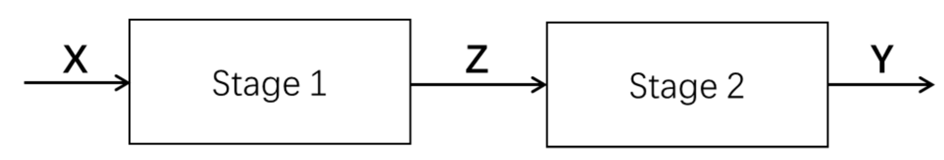
2. Two-Stage Process

To present our approach, we use the following notation:

$j\in J=1,2,\dots ,n$: The index of n DMUs.

$j_0\in J$: Denotes the evaluated DMU.

$X_j=\left(x_{ij},i=1,2,\dots ,m\right)$: The vector of the initial inputs used by $DM{U}_j$.

$Z_j=\left(z_{pj},p=1,2,\dots ,q\right)$: The vector of the intermediate measures for $DM{U}_j$.

$Y_j=\left(y_{rj},r=1,2,\dots ,s\right)$: The vector of the final outputs produced by $DM{U}_j$.

$v=\left(v_1,v_2,\dots ,v_m\right)$: The vector of weights for the initial inputs.

$w=\left(w_1,w_2,\dots ,w_q\right)$: The vector of weights for the intermediate measures.

$u=\left(u_1,u_2,\dots ,u_s\right)$: The vector of weights for the final outputs.

$e_{j_0}$: The overall efficiency of $DM{U}_{j_0}$.

$e_{j_0}^1$: The stage 1 efficiency for $DM{U}_{j0}$.

$e_{j_0}^2$: The stage 2 efficiency for $DM{U}_{j_0}$.

$e_{j_0}^{{\mathrm{k}}_{-}}$: The lower bound of stage-k efficiency for $DM{U}_{j_0}$, k = 1,2 while maintaining the overall efficiency $e_{j_0}$.

$e_{j_0}^{{\mathrm{k}}_{+}}$: The upper bound of stage-k efficiency for $DM{U}_{j_0}$, k = 1,2 while maintaining the overall efficiency $e_{j_0}$.

We consider the elementary two-stage system as represented in Figure 1, with each DMU transforming external inputs X into final outputs Y via intermediate measures Z by a two-stage process. In this basic setting, only external inputs to the first stage enter the system, and only outputs to the second stage leave the system. Supposing there are n DMUs in the system, we would typically define the efficiency of the first stage and second stage to $DM{U}_j$ as follows:

$$e_j^1=\frac{w{Z}_j}{v{X}_j},e_j^2=\frac{u{Y}_j}{\tilde{w}{Z}_j}.$$

(1)

Notice that, theoretically, the multipliers $w$ and $\tilde{w}$ for the intermediate measures do not have to be equal in efficiency evaluation. However, DEA researchers have broadly agreed that the same intermediate product $Z$ has the same multipliers associated with it in modeling network DEA, no matter whether it plays the role of inputs or outputs. In this article, we thus assume $w=\tilde{w}$.

The overall efficiency of the two-stage process is defined by the following relational model [3], which is the product of the stage efficiencies:

$$\begin{array}{l}\mathrm{Max}{\mathrm{e}}_{j_0}={\mathrm{e}}_{j_0}^1\cdot {\mathrm{e}}_{j_0}^2=\frac{u{Y}_{j_0}}{v{X}_{j_0}}\\ s.t.\\ \frac{w{Z}_j}{v{X}_j}\le 1;\frac{u{Y}_j}{w{Z}_j}\le 1,j=1,2,\dots ,\mathrm{n}\\ v,w,u\ge \epsilon \end{array}$$

(2)

where $\epsilon$ is a non-Archimedean constant. Further discussion about $\epsilon$ can be found in Amin and Toloo [25].

Equation (2) represents fractional programming, and can be transformed to linear programming by applying the Charnes‒Cooper transformation [26]. After the overall efficiency is achieved, the stage efficiencies can be calculated via Equation (1). Due to the existence of multiple optimal solutions in a linear program, it may lead to non-uniqueness for sub-stage efficiencies when decomposing the overall efficiency into stage efficiencies. The unique stage efficiency is important both in theory and in practice. This paper develops a rank-based method to achieve unique stage efficiency. For the purpose of comparison between the new approach and previous ones, the following section demonstrates several geometric properties of the Pareto front to simplify the uniform efficiency distribution method proposed by Liang et al. [19].

3. Geometric Properties of Pareto Front

The geometric properties of the Pareto front are the keystone for developing the new approach of efficiency decomposition and simplifying the uniform efficiency distribution. In order to elaborate our purpose, we consider a bi-objective program to be as follows:

$$\begin{array}{l}Max\frac{w{Z}_0}{v{X}_0}\\ \mathrm{Max}\frac{u{Y}_0}{w{Z}_0}\\ s.t.\\ \frac{w{Z}_j}{v{X}_j}\le 1;\frac{u{Y}_j}{w{Z}_j}\le 1,j=1,2,\dots ,\mathrm{n}\\ v,w,u\ge \epsilon \end{array}$$

(3)

Let $S$ be the variable space in Equation (3). The functions of stage efficiency, $e_{j_0}^1=\frac{w{Z}_{j_0}}{v{X}_{j_0}},e_{j_0}^2=\frac{u{Y}_{j_0}}{w{Z}_{j_0}}$ map variable space $S$ to the efficiency space (objective function space) in two-dimensional Euclidean space, denoted as $\Gamma$. Solving a multiple objective program means finding the efficient (Pareto optimal) solutions in variable space, which are mapped on the Pareto front in objective functions space, i.e., solutions that cannot be altered to increase the value of one objective function without decreasing the value of at least one other objective function. There are multiple approaches to solve the bi-objective program in Equation (3). However, the purpose here is not to solve Equation (3), but the geometric property of the Pareto front. In the following, we will prove that the Pareto front of the bi-objective program in Equation (3) is a bounded and continuous curve in the objective functions space. In order to test this result, we will first need to prove another result about the variable space $S$. Note that, although the geometric properties of Pareto front are demonstrated based on the DMU under evaluation, they apply to any other DMUs. Without a loss of generality, we only consider the situation for the DMU under evaluation.

Lemma 1.

$v,w,u$ are variables in Equation (3); the variable space $S$ is a path connected and closed in Euclidean space.

Proof. 

See Appendix A.1.1. □

Theorem 1.

The Pareto front is a continuous and bounded curve in efficiency function space.

Proof. 

See Appendix A.1.2. □

In the process of this proof, we showed that one part of the boundary of the efficiency function space $\Gamma$ is exactly the same with the Pareto front of Equation (3). Due to the closeness of $\Gamma$, the corresponding boundary belongs to the efficiency function space $\Gamma$. Consequently, for any given point $\left(e_{j_0}^1,e_{j_0}^2\right)$ on the Pareto front, there is always a corresponding multiplier coefficient $\left(v,w,u\right)$ associated with it in variable space of Equation (3). Realizing this point is important in developing the new efficiency decomposition approach and simplifying the uniform efficiency distribution method proposed in Liang et al. [1].

4. Rank-Based Efficiency Decomposition Approach

In this section, we redefine fairness based on efficiency rank and develop a rank-based efficiency decomposition approach.

In the basic two-stage setting, only the inputs to the first stage enter the system and only the outputs of the second stage leave the system. To calculate the system efficiency, the most representative approaches are the centralized model proposed by Liang et al. [19] and the relational model by Kao and Hwang [20], which are proven to be equivalent. Essentially, both of these models require the stages to compromise with each other in order to maximize overall efficiency. Making compromises implies that stage 1 and stage 2 cannot obtain the most favorable weights to achieve their respective advantages. The advantages of each stage can only be demonstrated when the stage efficiencies are calculated by a standard DEA model that allows each stage to achieve the best efficiency without compromises. After the overall efficiency is achieved, stage efficiencies can be obtained by decomposing the overall efficiency. When the optimal weights are not unique, non-uniqueness in decomposing the overall efficiency between the two stages may exist. To correctly and effectively identify the source of inefficiency inside DMUs, it is important to decompose the overall efficiency fairly and reasonably. We think that a fair and reasonable efficiency decomposition should meet two basic rules: (1) the decomposed stage efficiencies should objectively reflect the advantages of each stage; (2) the decomposed stage efficiencies should lie on the Pareto front. The first rule requires the decomposed stage efficiencies to maintain the relative advantages between two stages. The second rule requires that the corresponding multipliers to the decomposed stage efficiencies are Pareto optimal solutions. In what follows, we propose an efficiency decomposition approach to satisfy rules 1 and 2.

By applying the standard two-stage DEA model, we can obtain the efficiency score of each stage and its corresponding rank. Note that it is meaningless to compare the efficiency scores between the two stages. Although the efficiency of stage 1 for $DM{U}_{j_0}$ is greater than that of stage 2, it does not mean that stage 1 performs better than stage 2. However, we can estimate the relative advantages for each stage by rank. For example, the efficiency score of stage 2 is higher than that of stage 1, thus we can judge that stage 2 has advantages relative to stage 1. Therefore, we should bear in mind the relative advantages of the two stages when conducting an efficiency decomposition.

Specifically, for a given $DM{U}_{j_0}$, we can calculate the relative rate of increase of the efficiency rank for stage 1 and stage 2:

$$\alpha \%=\{\begin{array}{l}\frac{\mathrm{rank}(stage2)-rank(stage1)}{rank(stage2)},rank(stage2)\ge rank(stage1)\\ \frac{\mathrm{rank}(stage1)-rank(stage2)}{rank(stage1)},rank(stage1)>rank(stage2)\end{array}.$$

(4)

We use the CCR model to calculate the efficiency rank in this article.

Without a loss of generality, suppose that stage 1 ranks higher than stage 2, i.e., $rank(stage2)>rank(stage1)$, then the efficiency adjustment of stage 1 should be given priority. Specifically, the efficiency adjustment of stage 2 relative to stage 1 should be proportional to the relative increase rate of efficiency rank of stage 1 relative to stage 2, i.e.,

$$\frac{e_{j_0}^{2+}-e_{j_0}^2}{e_{j_0}^{2+}}-\frac{e_{j_0}^{1+}-e_{j_0}^1}{e_{j_0}^{1+}}=M\cdot \alpha \%\left(\frac{e_{j_0}^{1+}-e_{j_0}^1}{e_{j_0}^{1+}}\right),$$

(5)

where M is a positive constant number and $\alpha \%$ is the relative rate of increase in Equation (4). Equation (5) can be written equivalently as follows:

$$\frac{e_{j_0}^{2+}-e_{j_0}^2}{e_{j_0}^{2+}}=\left(1+M\cdot \alpha \%\right)\left(\frac{e_{j_0}^{1+}-e_{j_0}^1}{e_{j_0}^{1+}}\right).$$

(6)

Equation (6) is equivalent to the following expression:

$$\frac{e_{j_0}^{2+}-e_{j_0}^2}{e_{j_0}^{1+}-e_{j_0}^1}=\left(1+M\cdot \alpha \%\right)\cdot \frac{e_{j_0}^{2+}}{e_{j_0}^{1+}}.$$

(7)

Equation (7) implies that this proposed efficiency decomposition method finds a point $\left(e_{j_0}^1,e_{j_0}^2\right)$ on the Pareto front such that the slope of the line that crosses $\left(e_{j_0}^1,e_{j_0}^2\right)$ and $\left(e_{j_0}^{1+},e_{j_0}^{2+}\right)$ is $\left(1+M\cdot \alpha \%\right)\cdot e_{j_0}^{2+}/e_{j_0}^{1+}$. According to Theorem 1, the Pareto front is a continuous and bounded curve with two endpoints $\left(e_{j_0}^{1,L},e_{j_0}^{2,U}\right)$ and $\left(e_{j_0}^{1,U},e_{j_0}^{2,L}\right)$. The slope of the line that crosses $\left(e_{j_0}^{1+},e_{j_0}^{2+}\right)$ and point P ranges from 0 to positive infinity when point P moves from the point $\left(e_{j_0}^{1_{-}},e_{j_0}^{2_{+}}\right)$ to $\left(e_{j_0}^{1_{+}},e_{j_0}^{2_{-}}\right)$ on the Pareto front. Thus, given the parameter values of $M$ and $\alpha$, such a combination of efficiency decomposition $\left(e_{j_0}^1,e_{j_0}^2\right)$ must exist.

Note that $e_{j_0}=e_{j_0}^1\cdot e_{j_0}^2=e_{j_0}^{2+}\cdot e_{j_0}^{1_{-}}$, so Equation (7) can be transformed into

$$\frac{1+M\cdot \alpha \%}{e_{j_0}^{1+}}{\left(e_{j_0}^1\right)}^2-M\cdot \alpha \%\cdot e_{j_0}^1-e_{j_0}^{1_{-}}=0.$$

(8)

Consider a special case of $\alpha =0$, implying that the efficiency rank of stage 1 equals that of stage 2. In such a situation, stage 1 and stage 2 have the same relative advantages. Thus, the decomposition of stage efficiencies should be treated equally. From Equation (8), we can easily calculate the stage efficiencies when $\alpha =0$, i.e.,

$$e_{j_0}^1=\sqrt{e_{j_0}^{1+}\cdot e_{j_0}^{1_{-}}},e_{j_0}^2=\sqrt{e_{j_0}^{2+}\cdot e_{j_0}^{2_{-}}}.$$

(9)

This result exactly coincides with Zhou et al. [23], which implies that the Nash game decomposition method is a special case for the rank-based decomposition method. Furthermore, we will show that it is also the same as Liang et al. [19] in the next section, after model simplification. Equation (9) implies that the stage efficiency is the geometric mean of the upper and lower bound of the corresponding stage retaining the overall efficiency $e_{j_0}$ if the two stages are treated equally. For the general situation $\alpha >0$, we can obtain the stage efficiencies via solving Equation (8), i.e.,

$$e_{j_0}^1=\left[M\cdot \alpha \%+\sqrt{{\left(M\cdot \alpha \%\right)}^2+4\cdot e_{j_0}^{1_{-}}\cdot \frac{1+M\cdot \alpha \%}{e_{j_0}^{1+}}}\right]/2\cdot \frac{1+M\cdot \alpha \%}{e_{j_0}^{1+}},e_{j_0}^2=\frac{e_0}{e_{j_0}^1}.$$

(10)

From Equation (6), it is easy to conclude that ${\mathrm{e}}_{j_0}^1\in [{\mathrm{e}}_{j_0}^{1_{-}},{\mathrm{e}}_{j_0}^{1+}]$, which naturally leads to ${\mathrm{e}}_{j_0}^2\in [{\mathrm{e}}_{j_0}^{2_{-}},{\mathrm{e}}_{j_0}^{2+}]$. Therefore, the solution $\left(e_{j_0}^1,e_{j_0}^2\right)$ is a Pareto optimal solution, bounded between two points $\left(e_{j_0}^{1_{-}},e_{j_0}^{2+}\right)$ and $\left(e_{j_0}^{1+},e_{j_0}^{2_{-}}\right)$. In terms of the conclusion of Theorem 1, the Pareto front is a continuous curve in efficiency function space, and all Pareto solutions formed by Equation (1) lie on this Pareto front. There has to be a set of weights in variable space corresponding to the solution $\left(e_{j_0}^1,e_{j_0}^2\right)$. Consequently, the proposed decomposition method of stage efficiency meets the requirements of rules 1 and 2, which implies that the new decomposition method is valid.

5. Comparison of Different Efficiency Decomposition Methods

This section establishes the relationships between different efficiency decomposition methods. First, we show that the priority decomposition method can be derived from our model. Second, we simplify the uniform efficiency decomposition method proposed by Liang et al. [1] and conclude that it is a special case of our model. As a result, we show the equivalence between the uniform decomposition method and the priority decomposition method.

5.1. Priority Decomposition Method

To better understand the proposed method, we draw a sketch of a Pareto front based upon its geometric property, as depicted in Figure 2. The coordinates of points A and D represent the stage efficiencies calculated via a decentralized model, where stage 2 and stage 1 are treated as the respective leaders. Note that the stage efficiencies $e_{j_0}^{k_{-}}$ and $e_{j_0}^{k_{+}}$ are the lower and upper bound, respectively, of stage-k efficiency for $DM{U}_{j_0}$, k = 1,2, while maintaining the overall efficiency $e_{j_0}$. The coordinates of the points B and C represent the stage efficiencies, calculated via the priority method while maintaining the overall efficiency $e_{j_0}$. Notice that each point on the curve BC maximizes the overall efficiency of the relational model. Point B is identical to point C if the decomposition of stage efficiency is unique.

Reconsider Equation (7) $e_{j_0}^{2+}-e_{j_0}^2/e_{j_0}^{1+}-e_{j_0}^1=\left(1+M\cdot \alpha \%\right)\cdot e_{j_0}^{2+}/e_{j_0}^{1+}$. Note that the left-hand side of Equation (7) stands for the slope of the line that crosses the points $\left(e_{j_0}^1,e_{j_0}^2\right)$ and $\left(e_{j_0}^{1+},e_{j_0}^{2+}\right)$. The right-hand side is an adjusted slope based on the line that crosses the origin and the point $\left(e_{j_0}^{1+},e_{j_0}^{2+}\right)$, and the adjusted coefficient is $1+M\cdot \alpha \%$. From a geometric perspective, the essence of the newly proposed decomposition method in the current paper is to find a point $\left(e_{j_0}^1,e_{j_0}^2\right)$ on the Pareto front such that the slope of the line that crosses the point $\left(e_{j_0}^1,e_{j_0}^2\right)$ and $\left(e_{j_0}^{1+},e_{j_0}^{2+}\right)$ is $\left(1+M\cdot \alpha \%\right)\cdot e_{j_0}^{2+}/e_{j_0}^{1+}$. Since the parameter $\alpha$ is entirely determined by the relative rank of the two stages, the adjusted coefficient only depends on the parameter $M$. We can clearly see that the effect of $M$ with a value of 0 on stage efficiency decomposition is the same when $\alpha$ takes a value of 0 with the corresponding point being $e_{j_0}^1=\sqrt{e_{j_0}^{1+}\cdot e_{j_0}^{1_{-}}},e_{j_0}^2=\sqrt{e_{j_0}^{2+}\cdot e_{j_0}^{2_{-}}}$. As the value of $M$ increases, the point $\left(e_{j_0}^1,e_{j_0}^2\right)$ moves to the right along the Pareto front. Specifically, as the value of $M$ goes to positive infinity, the point $\left(e_{j_0}^1,e_{j_0}^2\right)$ will become the limit point $\left(e_{j_0}^{1_{+}},e_{j_0}^{2_{-}}\right)$. This result can be analytically obtained by making $M\to +\infty$ in Equation (10), i.e.,

$$\begin{array}{l}\underset{M\to +\infty }{\lim }{e}_{j_0}^1=\underset{M\to +\infty }{\lim }\left(\left[M\cdot \alpha \%+\sqrt{{\left(M\cdot \alpha \%\right)}^2+4\cdot e_{j_0}^{1_{-}}\cdot \frac{1+M\cdot \alpha \%}{e_{j_0}^{1+}}}\right]/2\cdot \frac{1+M\cdot \alpha \%}{e_{j_0}^{1+}}\right)\\ =\underset{M\to +\infty }{\lim }\left(2M\cdot \alpha \%/2\cdot \frac{1+M\cdot \alpha \%}{e_{j_0}^{1+}}\right)=e_{j_0}^{1_{+}}\end{array}$$

(11)

This result is an exact priority decomposition, which is achieved through assuming the first stage has priority while retaining the overall efficiency $e_{j_0}$. Each value of $M$ corresponds to a point that lies on the Pareto front between the points $\left(\sqrt{e_{j_0}^{1+}\cdot e_{j_0}^{1_{-}}},\sqrt{e_{j_0}^{2+}\cdot e_{j_0}^{2_{-}}}\right)$ and $\left(e_{j_0}^{1_{+}},e_{j_0}^{2_{-}}\right)$. We could take the parameter $M$ as the decision-maker’s preference, and $M=0$ reflects that the decision-maker treats two stages equally; $M>0$ indicates that the decision-maker prefers the stage with higher rank; $M\to +\infty$ represents the decision-maker giving absolute priority to the stage with a higher rank.

Similarly, another type of priority decomposition can be achieved through $M$ taking the value of positive infinity if the rank of stage 2 is higher than that of stage 1, i.e., $\left(e_{j_0}^1,e_{j_0}^2\right)=\left(e_{j_0}^{1_{-}},e_{j_0}^{2_{+}}\right)$. These two kinds of limited value scenarios imply that the newly proposed method in this paper includes the priority decomposition method as a special case.

5.2. Uniform Efficiency Decomposition Method

As in the current paper, a two-stage series process was under consideration in Liang et al. [19]’s paper. In order to calculate the overall efficiency of the two-stage process, a centralized model was proposed in their paper. The centralized model is equivalent in nature to the relational model proposed by Kao and Hwang [20]. In the centralized model, the overall efficiency is first obtained via maximizing the geometric mean of the two stages’ efficiency. The stage efficiencies are then calculated ex post. In cases of multiple optimal solutions that lead to non-uniqueness of $e_{j_0}^1$ and $e_{j_0}^2$, they developed a procedure to achieve an alternative distribution of $e_{j_0}^1$ and $e_{j_0}^2$ between the two stages. Specifically, they suppose that there exists a $\lambda$, $0\le \lambda \le 1$, such that

$$[\lambda e_{j_0}^{1_{-}}+(1-\lambda )e_{j_0}^{1_{+}}]\cdot [\lambda e_{j_0}^{2_{-}}+(1-\lambda )e_{j_0}^{2_{+}}]=e_{j_0}=e_{j_0}^{\mathrm{centralized}}.$$

(12)

Let ${\lambda }^{*}$ be the optimal solution of Equation (12); the stage efficiency distribution can be obtained as follows:

$$e_{j_0}^1={\lambda }^{*}{e}_{j_0}^{1_{-}}+(1-{\lambda }^{*})e_{j_0}^{1_{+}},e_{j_0}^2={\lambda }^{*}{e}_{j_0}^{2_{-}}+(1-{\lambda }^{*})e_{j_0}^{2_{+}}.$$

(13)

This procedure tests whether a set of weights is related to the efficiency distribution in Equation (12). If not, they need to find a set of weights and another efficiency distribution by solving a series of linear program problems to make sure the corresponding efficiency distribution is close to the distribution in Equation (12); see the details in Liang et al [19]. This procedure offers a perspective on how to fairly calculate stage efficiencies, but leads to complications for the calculation process, meaning it is not practical in many applications. Based on the continuity of the Pareto front, we can easily show that an efficiency distribution (Equation (12)) does exist that simplifies the calculation process of this procedure.

Looking at Figure 2, we can apply Cook, Liang, and Zhu [5]’s approach in a new way: to see whether a convex combination between the two points E and F exists such that the corresponding point lies on the Pareto front, that is

$$\lambda \left(e_{j_0}^{1_{-}},e_{j_0}^{2_{-}}\right)+\left(1-\lambda \right)\left(e_{j_0}^{1_{+}},e_{j_0}^{2_{+}}\right)=\left(\lambda e_{j_0}^{1_{-}}+\left(1-\lambda \right)e_{j_0}^{1_{+}}, \lambda e_{j_0}^{2_{-}}+\left(1-\lambda \right)e_{j_0}^{2_{+}}\right).$$

(14)

According to Figure 2, the answer is obvious, and point G is exactly the combination point. Since G is on the Pareto front, the corresponding weights exist naturally in the variable space. Furthermore, we can analytically provide the coordinates of G and the expression of $\lambda$. Consider the points $\left(e_{j_0}^{1_{-}},e_{j_0}^{2_{+}}\right)$ and $\left(e_{j_0}^{1_{+}},e_{j_0}^{2_{-}}\right)$, which both have the same overall efficiency, i.e.,

$${\mathrm{e}}_{j_0}=e_{j_0}^{1_{-}}\cdot e_{j_0}^{2_{+}}=e_{j_0}^{1_{+}}\cdot e_{j_0}^{2_{-}}.$$

(15)

Equivalently, we have $e_{j_0}^{2_{+}}/e_{j_0}^{1_{+}}=e_{j_0}^{2_{-}}/e_{j_0}^{1_{-}}=k$, which implies that points E and F have the same slope. Obviously, point G has the same slope as E and F. Let G’s coordinates be $\left(e_{j_0}^1,e_{j_0}^2\right)$, then we have

$$e_{j_0}^2/e_{j_0}^1=e_{j_0}^{2_{+}}/e_{j_0}^{1_{+}}=e_{j_0}^{2_{-}}/e_{j_0}^{1_{-}}=k\mathrm{and}{e}_{j_0}=e_{j_0}^1\cdot e_{j_0}^2.$$

(16)

From Equation (15), we can easily obtain

$$e_{j_0}^1=\sqrt{e_{j_0}^{1_{+}}\cdot e_{j_0}^{1_{-}}}\mathrm{and}{e}_{j_0}^2=\sqrt{e_{j_0}^{2_{+}}\cdot e_{j_0}^{2_{-}}}.$$

(17)

Note that $\lambda e_{j_0}^{1_{-}}+(1-\lambda )e_{j_0}^{1_{+}}=e_{j_0}^1=\sqrt{e_{j_0}^{1_{+}}\cdot e_{j_0}^{1_{-}}}$, $\lambda e_{j_0}^{2_{-}}+(1-\lambda )e_{j_0}^{2_{+}}=e_{j_0}^2=\sqrt{e_{j_0}^{2_{+}}\cdot e_{j_0}^{2_{-}}}$. Then we can obtain

$$\lambda =\frac{\sqrt{e_{j_0}^{1_{+}}}}{\sqrt{e_{j_0}^{1_{+}}}+\sqrt{e_{j_0}^{1_{-}}}}=\frac{\sqrt{e_{j_0}^{2_{+}}}}{\sqrt{e_{j_0}^{2_{+}}}+\sqrt{e_{j_0}^{2_{-}}}}=\frac{\sqrt{k}}{1+\sqrt{k}}.$$

(18)

So far, we have simplified and provided the analytical expressions for the efficiency distribution and stage efficiencies. From Equation (17), we can see that Liang et al. [19]’s model is a special case of our model when the parameter $M$ or $\alpha$ equals 0.

Different from the uniform efficiency decomposition, Zhou et al. [23] argued that a fair and reasonable method for efficiency decomposition is to make the two stages compete with each other to maximize their own efficiency when overall efficiency has been obtained under the cooperative game model. Surprisingly, we find that the result from Zhou et al. [23]’s model completely coincides with that in Liang et al. [19], which implies that the Nash bargaining game decomposition method is also a special case of our model.

In summary, our proposed model includes the three major efficiency decomposition methods as special cases. Furthermore, for any method of efficiency decomposition, it is necessary to find a point on the Pareto front such that the overall efficiency remains. Since we can always obtain a pair of given stage efficiency decompositions through adjusting the preference coefficient $M$, our newly proposed method is more general and incorporates other methods of efficiency decomposition into a unified framework.

6. Empirical Tests

In this section, we perform tests to demonstrate the applications of our model. Two separate tests are conducted to obtain the unique and reasonable stage efficiencies with data from the banking industry and the automobile industry.

6.1. Performance Evaluation of Banking

Efficiency evaluation in the banking industry has always been an important issue and received much attention [27,28,29,30]. For the purpose of comparison, we recalculate the case in Zhou et al. [23]. The authors applied the bargaining game model to determining the efficiency decompositions of 10 branches of China Construction Bank (CCB) in Anhui province, China (see Appendix A for the data). All the data are taken from the Annual Report [31] of China Construction Bank (CCB) in Anhui province. The processes of bank branches can be modeled as a two-stage system. In the first stage, employees (EMs), fixed assets (FAs), and expenses (EXs) are consumed to produce the outputs of credit (CR) and interbank loans (ILs). In the second stage, the outputs from the first stage are used as the inputs of the second stage to produce the outputs loan (Lo) and profit (PR).

The overall efficiency of the system is calculated by the relational model [20], and the second column in

Table 1. Efficiency scores for banks.

		Stage 1		Stage 2		Stage 1	Stage 2
DMU	Overall	${\mathbf{e}}^{1\_}$	${\mathbf{e}}^{1_{+}}$	${\mathbf{e}}^{2\_}$	${\mathbf{e}}^{2_{+}}$	CCR	CCR
1	1.0000	1.0000	1.0000	1.0000	1.0000	1.0000	1.0000
2	0.4344	0.5526	0.5541	0.7838	0.7861	0.5541	0.7861
3	0.2930	0.2930	0.4991	0.5869	1.0000	0.4991	1.0000
4	0.3013	0.3209	0.7593	0.3968	0.9389	0.7593	0.9699
5	0.3549	0.4304	0.7289	0.4869	0.8246	0.7289	0.8334
6	0.5448	0.5448	0.7359	0.7404	1.0000	0.7359	1.0000
7	0.1788	0.2881	0.5516	0.3242	0.6206	0.5516	0.6316
8	0.2818	0.3052	0.5325	0.5291	0.9232	0.5325	1.0000
9	0.3282	0.3845	0.5526	0.5939	0.8535	0.5526	1.0000
10	0.1747	0.3722	0.6498	0.2689	0.4695	0.6498	0.4979

lists all of the DMUs’ overall efficiency scores. Under the condition of retaining the overall efficiency, the lower and upper bound efficiency scores for stage 1 and stage 2 are presented in columns 3 to 6 in Table 1. Columns 7 and 8 give the standard efficiency scores for stage 1 and stage 2, as obtained by the CCR model. Since Liang et al. [19] and Zhou et al. [23]’s model lead to the same stage efficiency decompositions, we only demonstrate Zhou et al. [23]’s result for the purpose of comparison. As illustrated in

Table 2. BG model: efficiency scores and rankings.

	Stage 1	Stage 2	Stage 1	Stage 2
DMU	CCR	CCR	BG model	BG model
1	1(1)	1(1)	1.0000(1)	1(1)
2	0.5541(6)	0.7861(8)	0.5534(4)	0.785(3)
3	0.4991(10)	1(1)	0.3824(10)	0.7661(4)
4	0.7593(2)	0.9699(6)	0.4936(5)	0.6104(8)
5	0.7289(4)	0.8334(7)	0.5601(3)	0.6337(7)
6	0.7359(3)	1(1)	0.6332(2)	0.8605(2)
7	0.5516(8)	0.6316(9)	0.3987(9)	0.4485(9)
8	0.5325(9)	1(1)	0.4032(8)	0.6989(6)
9	0.5526(7)	1(1)	0.461(7)	0.749(5)
10	0.6498(5)	0.4979(10)	0.4918(6)	0.3553(10)
			RD = 10	RD = 20

, the second and third columns give standard efficiency scores for stage 1 and stage 2; the fourth and fifth columns present stage efficiencies for stage 1 and stage 2 according to Zhou et al. [23]’s model, which is the bargaining game model, abbreviated as “BG model” in Table 2. Similarly, the rank-based model proposed in this article is abbreviated as “R-B model” in

Table 3. R-B model: efficiency scores and rankings.

	Stage 1	Stage 2	Stage 1	Stage 2	Stage 1	Stage 2
DMU	M = 1	M = 1	M = 2	M = 2	M = 3	M = 3
1	1(1)	1(1)	1(1)	1(1)	1(1)	1(1)
2	0.5534(5)	0.7848(4)	0.5535(5)	0.7848(5)	0.5536(6)	0.7847(6)
3	0.3484(10)	0.841(3)	0.3326(10)	0.8808(3)	0.3237(10)	0.905(3)
4	0.5633(4)	0.5349(8)	0.6062(3)	0.497(8)	0.6343(2)	0.475(8)
5	0.5905(3)	0.601(7)	0.6123(2)	0.5796(7)	0.6284(3)	0.5648(7)
6	0.6081(2)	0.8959(2)	0.5939(4)	0.9173(2)	0.5848(4)	0.9316(2)
7	0.4068(8)	0.4396(9)	0.4142(8)	0.4317(9)	0.421(7)	0.4247(9)
8	0.3659(9)	0.7702(5)	0.3486(9)	0.8084(4)	0.3388(9)	0.8316(4)
9	0.4345(7)	0.7553(6)	0.4214(7)	0.7788(6)	0.4137(8)	0.7934(5)
10	0.5242(6)	0.3333(10)	0.5463(6)	0.3199(10)	0.562(5)	0.3109(10)
RD	6	18	6	16	4	17

and

Table 4. R-B model: efficiency scores and rankings.

	Stage 1	Stage 2	Stage 1	Stage 2	Stage 1	Stage 2
DMU	M = 4	M = 4	M = 5	M = 5	M = 6	M = 6
1	1(1)	1(1)	1(1)	1(1)	1(1)	1(1)
2	0.5536(6)	0.7846(6)	0.5536(6)	0.7846(6)	0.5537(6)	0.7845(6)
3	0.3181(10)	0.9211(3)	0.3141(10)	0.9326(3)	0.3113(10)	0.9412(3)
4	0.6539(2)	0.4608(8)	0.6682(2)	0.4509(8)	0.6792(2)	0.4436(8)
5	0.6407(3)	0.5539(7)	0.6504(3)	0.5456(7)	0.6583(3)	0.5392(7)
6	0.5785(4)	0.9417(2)	0.574(5)	0.9492(2)	0.5705(5)	0.955(2)
7	0.4272(7)	0.4186(9)	0.433(7)	0.413(9)	0.4382(7)	0.4081(9)
8	0.3326(9)	0.8471(4)	0.3284(9)	0.8582(4)	0.3252(9)	0.8664(4)
9	0.4086(8)	0.8033(5)	0.405(8)	0.8104(5)	0.4023(8)	0.8157(5)
10	0.5737(5)	0.3046(10)	0.5827(4)	0.2999(10)	0.5899(4)	0.2962(10)
RD	4	14	6	14	6	14

. The value of $\alpha$ can be easily calculated via the second and third columns in Table 1. For the purpose of comparison, we calculate six different sets of values of M for our model, as listed in Table 3 and Table 4, with all the corresponding ranks listed in parentheses.

From Table 2, only $DM{U}_1$ performs efficiently in both stages and the whole system. For the rest of the nine DMUs, non-uniqueness exists in the efficiency decomposition between two stages for each DMU since the maximal and minimal achievable efficiency scores for each stage are not the same. As explained in Section 4, a reasonable and fair efficiency decomposition method should maintain the relative advantages between the two stages. Hence, we focus the analysis of this empirical test on the rank differences.

As an example, we consider a special case, M = 4. We first consider the situation of the first stage. In Table 2, the second and fourth columns present the efficiency scores and corresponding ranks of stage 1, obtained by the CCR model and bargaining game model, respectively. The second column of Table 3 lists the results calculated by the rank-based model. Under the decomposition of the bargaining game model, only three DMUs have the same ranks as the standard CCR model, i.e., $DM{U}_1$, $DM{U}_3$ and $DM{U}_9$, but six DMUs for the rank-based model have the same rank, i.e., $DM{U}_1$, $DM{U}_2$, $DM{U}_3$, $DM{U}_4$, $DM{U}_8$ and $DM{U}_{10}$. For the rest of the DMUs, the bargaining game model has five DMUs with one rank difference, namely $DM{U}_5$, $DM{U}_6$, $DM{U}_7$, $DM{U}_8$ and $DM{U}_{10}$, but four DMUs for rank-based model, namely $DM{U}_5$, $DM{U}_6$, $DM{U}_7$, $DM{U}_9$. For the case of the two and three rank differences, the bargaining game model has $DM{U}_2$ and $DM{U}_4$, but there are none for the rank-based model.

If we define the absolute rank difference $RD$ as the sum of all rank differences, then we can calculate the rank difference of stage 1 for the bargaining game model and rank-based model as 10 and 4, respectively. Obviously, the lower the $RD$, the better the efficiency decomposition method works. From this standpoint, the newly proposed method with M = 4 works better than the bargaining game model.

A similar analysis can be applied to stage 2. From Table 2 and Table 4, we see that the bargaining game model and the rank-based model have four identical DMUs with zero rank difference, $DM{U}_1$, $DM{U}_5$, $DM{U}_7$, $DM{U}_{10}$. For the case of one rank difference, the two decomposition methods have the same result, namely $DM{U}_6$. For the case of two rank differences, the bargaining game model has $DM{U}_4$ and the rank-based model has $DM{U}_2$, $DM{U}_3$ and $DM{U}_4$. Notice that $DM{U}_3$ has a difference of three ranks and $DM{U}_2$ has five under the bargaining game model. For $DM{U}_8$ and $DM{U}_9$, the rank differences of the bargaining game model are 5 and 4, while those of the rank-based model are 3 and 4, respectively. Similarly, we can calculate that the absolute rank difference of stage 2, and the $RD$ (stage 2) of the bargaining game model and rank-based model are 20 and 14, respectively. Accordingly, the total rank difference of the bargaining game model and rank-based model are 30 and 18, respectively. The rank-based model works better for maintaining the relative advantages between two stages. Note that the rank difference of stage 2 is significantly greater than for stage 1, probably due to the efficient DMUs in stage 2 being significantly greater than in stage 1. We rank all the efficient DMUs of stage 2 as one, meaning that the rank difference lacks discrimination.

For different values of M, the total rank difference is $RD$ (M = 1) = 24, $RD$ (M = 2) = 22, $RD$ (M = 3) = 21, $RD$ (M = 5) = 20, $RD$ (M = 6) = 20. From the numerical results, we see that there is an inverted U-shaped relationship between the total rank difference and M. However, we cannot find an optimal value of M for the rank-based model, which is a shortcoming of this paper.

6.2. Performance Evaluation of Sustainable Designs

In recent years, sustainable design or, sometimes equivalently, design for the environment, has been considered as one of the most important practices for achieving sustainability. In this section, we apply the two-stage DEA framework for the sustainable design performance evaluation proposed in Chen at al. [18], which uses design efficiency as a performance measure to evaluate how well multiple product specifications and attributes are combined in a product design to achieve better environmental performance. Contrary to the traditional measures for sustainable design, which mostly focus on the absolute environmental performance, this two-stage DEA model includes an “industrial design stage” (stage 1) and a “bio design stage” (stage 2) in order to identify the most efficient way to combine the product specifications and attributes to achieve better environmental performance through product design.

The testing data are collected from the 2013 vehicle emissions testing database published by the U.S. EPA [32], which includes valid data on 12 new models introduced by three different manufacturers (see Appendix A for the original data). In the two-stage DEA model, cubic inch displacement (cid), rated horsepower (rhp), engine speed versus vehicle speed at 50 mph (n/v ratio), and axle ratio (axle) are treated as the inputs; equivalent test weight (etw) and fuel economy (mpg) as the intermediates; and hydrocarbon emissions (hc), carbon monoxide emissions (CO), carbon dioxide emissions ($C{O}_2$), and nitrogen oxide emission ($N{O}_{\mathrm{x}}$) as outputs. Note that higher levels of outputs usually indicate better performance in DEA. Thus, we treat the reciprocals of cubicinch displacement, rated horsepower, compression ratio, and equivalent test weights in our analysis to fit the DEA use.

The results are listed in

Table 5. Efficiency scores for sustainable design.

		Stage 1		Stage 2		Stage 1	Stage 2
DMU	Overall	${\mathbf{e}}^{1\_}$	${\mathbf{e}}^{1_{+}}$	${\mathbf{e}}^{2\_}$	${\mathbf{e}}^{2_{+}}$	CCR	CCR
1	0.8891	0.9475	0.9633	0.9229	0.9383	0.9475	1
2	0.8127	0.9295	0.9295	0.8742	0.8742	0.9735	1
3	0.9171	0.9171	0.9171	1	1	1	0.9951
4	1	1	1	1	1	1	1
5	0.8791	0.9295	0.9295	0.9457	0.9457	1	1
6	0.8134	1	1	0.8134	0.8134	1	1
7	0.7593	0.9413	0.9413	0.8067	0.8067	1	0.99
8	0.7119	1	1	0.7119	0.7119	1	0.9787
9	0.7579	1	1	0.7579	0.7579	1	0.986
10	0.7134	0.9734	0.9734	0.7328	0.7328	0.9741	0.996
11	0.9291	0.98	0.98	0.9481	0.9481	1	1
12	0.6552	0.8958	0.8958	0.7314	0.7314	0.9456	0.9924

. The second column presents the overall efficiencies based on the two-stage DEA model. Under the condition of retaining the overall efficiency, the lower and upper bound efficiencies of stage 1 and stage 2 are listed in columns 3 to 6. The last two columns list the CCR efficiency scores of stage 1 and stage 2, respectively. According to the unique test procedure proposed in Liang et al [19], all DMUs have unique stage efficiencies except $DM{U}_1$ since its lower and upper bound efficiencies are not equal. Based on the rank of stage 1 and stage 2 determined by its CCR efficiency scores, we can easily calculate the value of $\alpha$, which equals 90.91%.

Table 6. Efficiency decomposition: R-B model vs. BG model.

	R-B model
DMU1	Stage 1	Stage 2	RD
M = 1	0.9529	0.9330	8
M = 2	0.9517	0.9343	8
M = 3	0.9509	0.9350	8
M = 4	0.9503	0.9356	8
BG model	0.9554	0.9306	8

lists four sets of efficiency scores for stage 1 and stage 2, which are calculated by a rank-based model. The stage efficiencies calculated by the bargaining model are presented in the last row. The last column of Table 6 shows that both the rank-based model and the bargaining game model have the same rank differences, which implies that the two models work identically in this case. The reason is that only $DM{U}_1$ needs an efficiency decomposition, and there are no other DMUs whose stage efficiencies are between the lower bound and upper bound of $DM{U}_1$. Therefore, no matter how the values of M are selected, there is no impact on the rankings.

7. Concluding Remarks

Efficiency decomposition can help decision-makers to establish the inefficient source so that appropriate efforts can be devoted to improving performance. To discover the internal inefficiencies, the overall efficiency of the whole system needs to be decomposed into stage efficiencies. Due to the non-unique optimal weights of a linear program, non-uniqueness in efficiency decomposition may exist. Three major efficiency decomposition methods have been proposed: Liang et al. [19]’s uniform efficiency distribution model, Zhou et al. [23]’s bargaining game model, and Kao and Hwang [20]’s priority decomposition model. Each model has a different perspective on efficiency decomposition and claims to achieve fair, reasonable, and unique stage efficiencies. However, the foundations of these models are totally different, which can make it harder for researchers and practitioners to establish their relative superiority. Through proving the continuity of the Pareto front in efficiency function space, we simplified Liang et al. [19]’s model, and found that the efficiency decompositions derived by Cook, Liang, and Zhu [5] and Zhou et al. [23]’s models are the same. Furthermore, based on this geometric property of the Pareto front, we propose a rank-based model to achieve reasonable and unique efficiency decompositions for each stage. The proposed rank-based model allows for the three abovementioned models to be treated as special cases. Liang et al. [19] and Zhou et al. [23]’s models, which were proven to be equivalent, can be unified into the rank-based model as a special case when $\alpha$ or M equals 0. Kao and Hwang [20] can also be included as a special case when M takes the value of positive infinity. As presented, there are two parameters in our model, $\alpha$ and M. The parameter $\alpha$ reflects the relative advantages between two sub-stages, which means the efficiency decomposition can be conducted fairly and reasonably. In practice, another parameter M can be viewed as the preference of the decision-maker. Theoretically, our model can also include any other efficiency decomposition models as special cases as long as the value of the decision-maker’s preferred coefficient M is adjusted appropriately. Thus, the proposed rank-based model provides a unified perspective for investigating different efficiency decomposition methods, as well as a better understanding of the existing efficiency decomposition approaches in the literature. However, the optimal values of M for our model have not been achieved in this current paper. As an example, only a few sets of special values of M are presented to demonstrate the applications of our model. The reason is that the optimal values of M for our model are DMU-specific, and the calculation is too complicated. This is a drawback of this study.

Lastly, the proposed model was applied to evaluate bank performance and the efficiency of sustainable product design in the automobile industry. In the banking evaluation, non-uniqueness of efficiency decomposition occurs in nine out of 10 banks. For the purpose of comparison, the bargaining game and rank-based models are used in this case. Through defining the rank differences, we compared the results of efficiency decomposition derived by these two models. It turns out that our model performance is better than the bargaining model. In a second test, we showed the applicability of our model to the evaluation of sustainable product design in the automobile industry. There are 12 types of vehicles from three different manufacturers included in this case. Only one DMU has the problem of non-uniqueness of efficiency decomposition. We used the rank-based model to achieve unique stage efficiencies. For the purpose of comparison, we also calculated the results by the bargaining model. Since the rank differences would not make any difference no matter whether the rank-based model or bargaining model is used in this case, these two models perform equally well. In addition, although our model was proposed based on the most fundamental two-stage network process, the idea introduced here applies to other types of network DEA model.

References

1. Charnes, A.; Cooper, W.; Rhodes, E. Measuring the efficiency of decision making units. Eur. J. Oper. Res. 1978, 2, 429–444. [Google Scholar] [CrossRef]
2. Kou, G.; Peng, Y.; Wang, G. Evaluation of clustering algorithms for financial risk analysis using MCDM methods. Inf. Sci. 2014, 275, 1–12. [Google Scholar] [CrossRef]
3. Li, G.; Kou, G.; Peng, Y. A Group Decision Making Model for Integrating Heterogeneous Information. IEEE Trans. Syst. Man, Cybern. Syst. 2018, 48, 982–992. [Google Scholar] [CrossRef]
4. Zhang, H.; Kou, G.; Peng, Y. Soft consensus cost models for group decision making and economic interpretations. Eur. J. Oper. Res. 2019, 277, 964–980. [Google Scholar] [CrossRef]
5. Cook, W.D.; Liang, L.; Zhu, J. Measuring performance of two-stage network structures by DEA: A review and future perspective. Omega 2010, 38, 423–430. [Google Scholar] [CrossRef]
6. Halkos, G.E.; Tzeremes, N.G.; Kourtzidis, S.A. A unified classification of two-stage DEA models. Surv. Oper. Res. Manag. Sci. 2014, 19, 1–16. [Google Scholar] [CrossRef]
7. Chen, Y.; Cook, W.D.; Li, N.; Zhu, J. Additive efficiency decomposition in two-stage DEA. Eur. J. Oper. Res. 2009, 196, 1170–1176. [Google Scholar] [CrossRef]
8. Färe, R.; Grosskopf, S. Productivity and intermediate products: A frontier approach. Econ. Lett. 1996, 50, 65–70. [Google Scholar] [CrossRef]
9. Du, J.; Liang, L.; Chen, Y.; Cook, W.D.; Zhu, J. A bargaining game model for measuring performance of two-stage network structures. Eur. J. Oper. Res. 2011, 210, 390–397. [Google Scholar] [CrossRef]
10. Seiford, L.M.; Zhu, J. Profitability and Marketability of the Top 55 U.S. Commercial Banks. Manag. Sci. 1999, 45, 1270–1288. [Google Scholar] [CrossRef] [Green Version]
11. Zhu, J. Multi-factor performance measure model with an application to Fortune 500 companies. Eur. J. Oper. Res. 2000, 123, 105–124. [Google Scholar] [CrossRef]
12. Mardani, A.; Zavadskas, E.K.; Streimikiene, D.; Jusoh, A.; Khoshnoudi, M. A comprehensive review of data envelopment analysis (DEA) approach in energy efficiency. Renew. Sustain. Energy Rev. 2017, 70, 1298–1322. [Google Scholar] [CrossRef]
13. Sueyoshi, T.; Yuan, Y.; Goto, M. A literature study for DEA applied to energy and environment. Energy Econ. 2017, 62, 104–124. [Google Scholar] [CrossRef]
14. An, Q.; Wang, Z.; Ali, E.; Zhu, Q.; Zhu, X. Efficiency evaluation of parallel interdependent processes systems: An application to Chinese 985 Project universities. Int. J. Prod. Res. 2018, 1–13. [Google Scholar] [CrossRef]
15. Wu, J.; Zhu, Q.; Chu, J.; An, Q.; Liang, L. A DEA based approach for allocation of emission reduction tasks. Int. J. Prod. Res. 2016, 54, 5618–5633. [Google Scholar] [CrossRef]
16. Zhou, H.; Yang, H.; Chen, Y.; Zhu, J. Data envelopment analysis application in sustainability: The origins, development and future directions. Eur. J. Oper. Res. 2018, 264, 1–16. [Google Scholar] [CrossRef]
17. Hwang, S.-N.; Chen, C.; Chen, Y.; Lee, H.-S.; Shen, P.-D. Sustainable design performance evaluation with applications in the automobile industry: Focusing on inefficiency by undesirable factors. Omega 2013, 41, 553–558. [Google Scholar] [CrossRef]
18. Chen, C.; Zhu, J.; Yu, J.-Y.; Noori, H. A new methodology for evaluating sustainable product design performance with two-stage network data envelopment analysis. Eur. J. Oper. Res. 2012, 221, 348–359. [Google Scholar] [CrossRef]
19. Liang, L.; Cook, W.D.; Zhu, J. DEA models for two-stage processes: Game approach and efficiency decomposition. Nav. Res. Logist. 2008, 55, 643–653. [Google Scholar] [CrossRef]
20. Kao, C.; Hwang, S.-N. Efficiency decomposition in two-stage data envelopment analysis: An application to non-life insurance companies in Taiwan. Eur. J. Oper. Res. 2008, 185, 418–429. [Google Scholar] [CrossRef]
21. Kao, C. Efficiency decomposition and aggregation in network data envelopment analysis. Eur. J. Oper. Res. 2016, 255, 778–786. [Google Scholar] [CrossRef]
22. Kao, C. Efficiency decomposition for general multi-stage systems in data envelopment analysis. Eur. J. Oper. Res. 2014, 232, 117–124. [Google Scholar] [CrossRef]
23. Zhou, Z.; Sun, L.; Yang, W.; Liu, W.; Ma, C. A bargaining game model for efficiency decomposition in the centralized model of two-stage systems. Comput. Ind. Eng. 2013, 64, 103–108. [Google Scholar] [CrossRef]
24. Li, H.; Chen, C.; Cook, W.D.; Zhang, J.; Zhu, J. Two-stage network DEA: Who is the leader? Omega 2018, 74, 15–19. [Google Scholar] [CrossRef]
25. Amin, G.R.; Toloo, M. A polynomial-time algorithm for finding ε in DEA models. Comput. Oper. Res. 2004, 31, 803–805. [Google Scholar] [CrossRef]
26. Charnes, A.; Cooper, W.W. Programming with linear fractional functionals. Nav. Res. Logist. Q. 1962, 9, 181–186. [Google Scholar] [CrossRef]
27. AlHassany, H.; Faisal, F. Factors influencing the internet banking adoption decision in North Cyprus: an evidence from the partial least square approach of the structural equation modeling. Financ. Innov. 2018, 4, 29. [Google Scholar] [CrossRef] [Green Version]
28. Tang, Y.; Moro, A.; Sozzo, S.; Li, Z. Modelling trust evolution within small business lending relationships. Financ. Innov. 2018, 4, 19. [Google Scholar] [CrossRef]
29. Asongu, S.A.; Odhiambo, N.M. Size, efficiency, market power, and economies of scale in the African banking sector. Financ. Innov. 2019, 5, 4. [Google Scholar] [CrossRef] [Green Version]
30. Kou, G.; Chao, X.; Peng, Y.; Alsaadi, F.E.; Herrera-Viedma, E. MACHINE LEARNING METHODS FOR SYSTEMIC RISK ANALYSIS IN FINANCIAL SECTORS. Technol. Econ. Dev. Econ. 2019, 1–27. [Google Scholar] [CrossRef]
31. China Construction Bank (Anhui Branch). Annual Report 2004 of China Construction Bank in Anhui Province. 2004. Available online: http://www.ccb.com/cn/uploads/1-26.1118369283972.pdf (accessed on 14 June 2019). (In Chinese).
32. United States Environmental Protection Agency. Certification Emission Test Data. 2013. Available online: https://www.epa.gov/ (accessed on 14 June 2019).
Figure 1. Two-stage system.
Sustainability 11 04401 g001
Figure 2. Pareto front.
Sustainability 11 04401 g002