An Integrated Global Food and Energy Security System Dynamics Model for Addressing Systemic Risk


1
Global Sustainability Institute, Anglia Ruskin University, Cambridge CB1 1PT, UK
2
Institute for Ecological Economics, Vienna University of Economics and Business (WU), 1020 Vienna, Austria
*
Author to whom correspondence should be addressed.
Sustainability 2019, 11(14), 3995; https://doi.org/10.3390/su11143995
Submission received: 6 June 2019
/
Revised: 12 July 2019
/
Accepted: 19 July 2019
/
Published: 23 July 2019
(This article belongs to the Special Issue Systems Approaches to Complex and Sustainable Food Systems)
Abstract
:In 1972, The Limits to Growth, using the World3 System Dynamics model, modeled for the first time the long-term risk of food security, which would emerge from the complex relation between capital and population growth within the limits of the planet. In this paper, we present a novel system dynamics model to explore the short-term dynamics of the food and energy system within the wider global economic framework. By merging structures of the World3, Money, and Macroeconomy Dynamics (MMD) and the Energy Transition and the Economy (ETE) models, we present a closed system global economy model, where growth is driven by population growth and government debt. The agricultural sector is a general disequilibrium productive sector grounded on World3, where capital investment and land development decisions are made to meet population food need, thus generating cascade demands for the energy and capital sector. Energy and Capital Sectors employ a more standard economic approach in line with MMD and ETE. By taking into account the role of financial, real, and natural capital, the model can be used to explore alternative scenarios driven by uncertainty and risk, such as climate extreme events and their impacts on food production. The paper presents scenario analysis of the impact of an exogenous price, production, and subsidies shock in the food and/or energy dimensions on the economic system, understanding the sources of potential cascade effects, thus providing a systemic risk assessment tool to inform global food security policies.
Keywords:
system dynamics; economy; energy; agriculture; subsidy policy; production shock; climate risk1. Introduction
The impact of climate change on global food systems is expected to be heterogeneous and uneven across regions in the world [1]. The last decade was already characterized by more frequent and disruptive weather events, which increased the social and economic costs of natural disasters [2,3]. However, while the physical causes of food production shocks are well analyzed, the dynamics of other sectors’ responses to them, and the implications on sustainable development and poverty reduction require further attention [4]. In a world characterized by an increase in population growth, in particular, in low-income and emerging countries [5], lack of timely policy responses could extend the scale of the food crisis and increase geopolitical instability.
Recently the World Resource Institute (WRI) found that to meet projected crop needs, given the expected population growth, through an increase in production and without expanding the annual area harvested, crop yields would need to grow by 32% more from 2006 to 2050 than they did from 1962 [6]. Additionally, they would need to see this increased growth without being able to fully benefit from the same scale of exploitation of new technologies (scientifically bred seeds and fertilizers) as in the past, as we are unlikely to see a second ‘green revolution’ and with water being more and more constrained. At the same time, the International Food Policy Research Institute (IFPRI) [7] found that climate change could reduce yields of irrigated wheat and rice by 30% and 15%, respectively (with geographic differences). For example, Mediterranean countries, Sub-Saharan Africa, and West Asia are more likely to be negatively affected in terms of yields, with important consequences on food security and malnutrition. Despite the uncertainties on estimates, the Fifth Assessment Report of the Intergovernmental Panel on Climate Change [8] states that the largest declines in crop yields are expected in tropical areas, with crop yields expected to decline by eight percent by the 2050s in South Asia and Africa. No change has been identified for rice, results for cassava are inconclusive, and yields of other major crops (e.g., sorghum and millet) are expected to decline significantly.
The interactions between weather shocks, food production, and households’ response have recently started to be analyzed [9,10]. For example, the increasing probability of occurrence and duration of extreme events could accrue social tensions, which might break down into conflicts through consequent impacts of price spikes, such as those experienced during the 2007–2008 food price shocks [11,12,13,14]. Lloyd’s [15] recognized that the expected increases in chronic pressure on food would increase the vulnerability of the food system to acute shocks, and the risk for the insurance industry in terms of potential losses from claims across multiple classes of insurance, from business interruption to agriculture, terrorism, and political risk.
Besides, there is increasing evidence of a connection between energy and food prices [16], especially with the increasing use of biofuels [17]. Therefore, new importance is given to agriculture and energy policies, which can no longer be taken separately in relation to increased food and oil price volatility, energy security ambitions, and environmental concerns [18].
The complexity and multidimensionality of the picture displayed above require that policies aimed at assuring food security need to account for the interconnectedness of the issues at stake within a sustainable and inclusive development framework, crossing the current sector barriers. The reason being that these interconnected issues present a banquet of multidimensional consequences (and development challenges) in terms of systemic characteristics and chain effects.
In this paper, we present a novel global food and energy system dynamics model to explore the short-term (1 to 5 years) interdependencies of food-energy commodity price volatility and the cascade effects on the real and financial economy. With the final aim of providing a systemic risk assessment tool to inform global food security policies, we argue that the current model is a first step in the understanding of the relationships between food and energy, and further work is necessary to address their systemic independencies. The model developed is a System Dynamics model, thus relying on continuous-time differential equations modeling, bounded rationality between economic agents, feedback loops, and time delays, and non-linear behavior. The model builds based on (i) the last version of the World3 (World3-03) [19], (ii) the Energy Transition and the Economy (ETE) Model [20], and (iii) Money and Macroeconomic Dynamics (MMD), as per Yamaguchi [21]. In particular, we model the agricultural sector based on World3. We assume that all agricultural commodities are transformed into a single crop [22] and rely on the Meadows et al. [19] for the model investments, land, and production equations. The resulting system is embedded in a simplified economic modeling framework, as taken from ETE [20]. This involves the relationship between labor, prices, interest rate, money supply, and financial flows. Except for the agricultural sector, we employ a Cobb-Douglas Production function and use an inventory structure perception delay structure in line with MMD [21]. We complete the structure with ad-hoc structures, including a division of households into capital owners and workers, and allow exogenous input to the model, such as household consumption and government debt creation.
We note important limitations to this model, most importantly, the aggregate nature of the model structure. As the focus of our modeling is to understand complex interconnections and feedbacks between different commodities by necessity, these have to be modeled at an aggregate level to be able to interpret the results within the context of informing policy. Therefore, we do not attempt to model individual commodities, such as wheat, maize, rice, or meat (at least in the initial model), or the interaction between them. We also cannot model the particular risks associated with the local nature of natural disasters or societal and market interactions. The supply chain within energy and food systems is also not modeled. However, these additional complexities are likely to increase the risks from the shocks that we model rather than reducing them.
Also, the limitations of this analysis include the feedback of biofuel production from food to satisfy energy demand, which has not been taken into account. Additionally, no renewable energy resource has been taken into account in the energy mix. Such inclusions could have altered the shock analysis in comparison to real data; however, as we are only interested in the immediate short-term, these assumptions were deemed appropriate at this time, given that they represented only a small portion of the global market historically. It is also likely that the production shocks in our scenarios, which are required to replicate real price data, will be higher than those observed in the real world. This will mainly be due to unmodeled aspects of the real world, including government, market, and individual behaviors involved in price setting (especially on international markets). There will also be several limitations due to the need to calibrate our scenarios on real-world data that are unavailable or imprecise (for example, global subsidies). Further work is needed to develop a more accurate understanding of global subsidies for fossil fuels and food, including those for exploration, research and development, cost of regulation and enforcement, environmental damage and clean up, and production [23,24,25]. The indirect costs of access to resources, such as those associated with geopolitical stability or war, are also not considered.
As a result, we focus our attention on the mutual feedback between food and energy at the global aggregate level. In particular, while food production requires energy for the production (thus embedded in the price of food as cost), the food price impacts overall price inflation, that, in turn, can affect the setting of energy price. We argue that modeling this complex interaction is a valuable addition to the process of policy development when running alongside other models, as it allows the feedbacks contained within the system interdependencies to be accounted for, which leads to the better understanding of the cascade effects associated with shocks to the system.
2. Modeling the Relation between Climate Risk and Agriculture
There is no agreement on the quantification of the impact of different drivers of climate change risk on food systems (in terms of magnitude and relative importance) at different geographic scales. This uncertainty is linked to the different nature of the effects of climate change on agriculture, being either:
- Direct, such as physical damage on crops, animals, and trees;
- Indirect, such as the loss of potential production and capacities, increased costs of production, the lower flow of goods and services;
- Tangible—that can be easily measured in monetary terms;
- Intangible—difficult to measure in monetary terms, such as the fear of future disruption, stress.
To fill in this knowledge gap over the last decade, agricultural and sector models were adapted to integrate the sources of uncertainty arising from changing climate [26]. Many activities under the Agricultural Model Intercomparison and Improvement Project (AGMiP) have provided important insights into the various sources of variability in model-to-model performance in such studies. At the moment, we can use several models to assess different impacts of climate change on agriculture – long-term changes, short-term responses to shocks, land use allocation, food production, prices, and carbon emissions [27,28].
However, the current sectorial models used to analyze food systems are not able to represent the complexity, non-linearity, and time-dependent nature of the issues at stake. Sector-specific or agricultural productivity models have several limitations for estimating climate change impacts on agriculture [29]. Integrated Assessment Models (IAM), in particular, do not adequately capture (i) the role of time lags between the imposition of a stress and how farmers (and markets) respond, which in complex dynamical systems may have a potentially destabilizing effect; (ii) time delays associated with how prices and agents respond immediately after a shock occurs (e.g., farmers adapting their investing or land allocation choices), time lags in prices perceptions (information delays) and land conversion in the case of farmers’ behavior (material delay); (iii) many IAM models have a long-term focus, which makes them less well-suited to some aspects of climate stresses, which may manifest themselves as a sequence of seasonal and annual events and to meet short-term policy demands [30].
The feedback loops that characterize the agents and sectors of the food systems, the amplification effects of a shock along the food value chains, and the time delays that characterize the imposition of a shock and their response to it, require models able to deal with non-linearity, uncertainty, and boom-and-burst cycles. In this paper, we argue that System Dynamics modeling is a suitable approach to deal with such a complex system and should be run alongside Integrated Assessment Models to develop a better understanding of the full food system risk.
System Dynamics (SD) is a modeling paradigm pioneered by Forrester [31] to study complex social systems and support decision making through the understanding of a system’s dynamics under different uncertain future scenarios. We rely on SD as suitable in modeling the price system and financial flows [21,32], as well as support scenario policy behavior analysis at the aggregate level of the global systems [33,34,35,36]. In particular, it allows the testing of which policies are more robust when specific scenarios emerge from simulations, and to capture counterintuitive, maybe undesired policy consequences [37].
In 1972, the “Limits to Growth” (LtG), commissioned by the Club of Rome, developed the World3 model to better understand these complex dynamics [19,35,38]. World3 showed the risk of overshoot due to human pressure on ecosystems and the end of growth. By representing a world system composed of land, non-renewable resources, capital, population, and persistent pollution, World3 clearly showed that, unless corrective actions are taken to drive the global system towards sustainability, persistent pollution, land erosion, or resource extraction would overshoot the limits of the planet at some point during the 21st century, causing significant impacts on population and capital, including the possibility of collapse. Nowadays, evidence [1,39,40] supports the view that there are planetary limits in certain systems, and a particular focus has been given to greenhouse gas emissions [41,42]. The dynamics of the World3 model have been recently found to be able to match with real-data [43].
In the development of this study, we argue understanding the dynamics of volatility in energy and food prices over the short- to medium-term is critical. Building on the Limits to Growth World3-03 model [19], we add the financial system, government, and the role of resource prices, based on the structures presented in two different but complementary SD models, i.e., the ETE model [20,32] and the MDM System [21]. Although accounting for the limits to growth in the land and non-renewable energy systems according to the World3-03, we propose an interpretation of the economic system similar to Sterman [20], that is a closed system structural economy composed of different productive sectors responsible for assuring the demand of each commodity (fossil fuels, food, goods, and capital), is met at any time in the simulation. Such an economy is constrained by natural resources (land and energy reserves), uses the capital for production activity, and endogenously generates commodity prices from the interaction between supply and demand for each of them, cost of production and inflationary effects. Prices are used to translate physical to financial flows, which are depicted using a balance sheet approach for each sector and are driven by a debt money system. A hypothetical global government sector is also captured in line with Yamaguchi [21]. As this approach is focused on the short-term, we substitute the Persistent Pollution dimension of World3 with exogenous shocks on the other dimensions [33,34,35,36]. The current design can depict complex emerging interactions among energy and food system dynamics and possible cascade impacts of food and energy production shocks on the rest of the economy, as well as testing subsidy policies to mitigate such an effect.
SD uses stocks, flows, feedback loops, and delays as key elements for the representation of complex systems. Such a perspective allows us to describe a feedback structure of the agriculture-energy, system nexus, and integrate it with the global economy, providing a complete closed money system based on business principles and natural resource use. Such a structure helps explain the non-linearity, which emerges from the dynamics of multi-level systems, such as financial, real, and natural, which are mutually interdependent at different levels of study. The model can be used to study shocks in the system, such as the effect of cutting subsidies to the agriculture sector or a production shock from extreme weather events.
In addition to this, SD allows the effective representation of both continuous (i.e., land erosion, gradual perception in demand change of an economy) as well as discrete processes (i.e., sudden investments change level, sudden shock in energy price). Stock variables in an SD are representative of inertial features in the system that cannot change instantaneously (stock of food ready for consumption, land used for producing cereals, overall debt in the economy). Flow variables instead represent the processes that work to change the state of a system (stocks), and in the case of a productive system that is governed by demand change they include, for example, the flow of production or consumption which change the stock of a product to be consumed, arable land developed as a result of investment in agriculture, or the rate of debt redemption from a productive sector to the financial sector.
SD represents a valuable alternative to current modeling approaches in agriculture, such as Integrated Assessment (IAM) and Sector-Specific Models.
3. The Model Framework
The model presented in this paper is a generic out of equilibrium closed system economy, distinguishing households (both workers—W and capital owners—H), firms (goods and capital—GC, energy—EN, and agriculture for cereal production—AC), public sector (government - GV and banking system—B), as seven macro-sectors aggregated at the level of the global economy. We use cereal production as a proxy for food production within the model as a good first approximation to food system risk, which allows easier coupling between land use and food output [9]. This allows us to look at the system from a top-down perspective and focus the entire analysis on the relationships between food and energy prices. Economic growth is driven by rising population and government debt creation and is supported by the debt-money system, which generates the liquidity required for trading resources over time. The model includes resource limits in terms of land availability (in AC sector) and fossil fuel reserves availability (in EN sector).
In the model, demand is generated at the real level of the economy but constrained by the finance available in each sector. The rise in population for each type of household multiplies an exogenous parameter, representing the desired consumption per capita per commodity. Due to the increase in consumption from households, every sector increases its stock of capital and, in turn, must consume more energy, thus determining a cascade demand across sectors. Desired orders of capital are then altered according to the availability of cash for each sector involved in the market using simple non-linear relationships, describing the behavior of decision-makers at the financial and operations levels while adjusting key control variables. By using a balance sheet approach [21], every transaction is recorded in the model four times (double-entry rule between assets and liabilities and recorded in two sectors per transaction). The model also endogenously calculates GDP and inflation using AC and GC production and energy consumption by households.
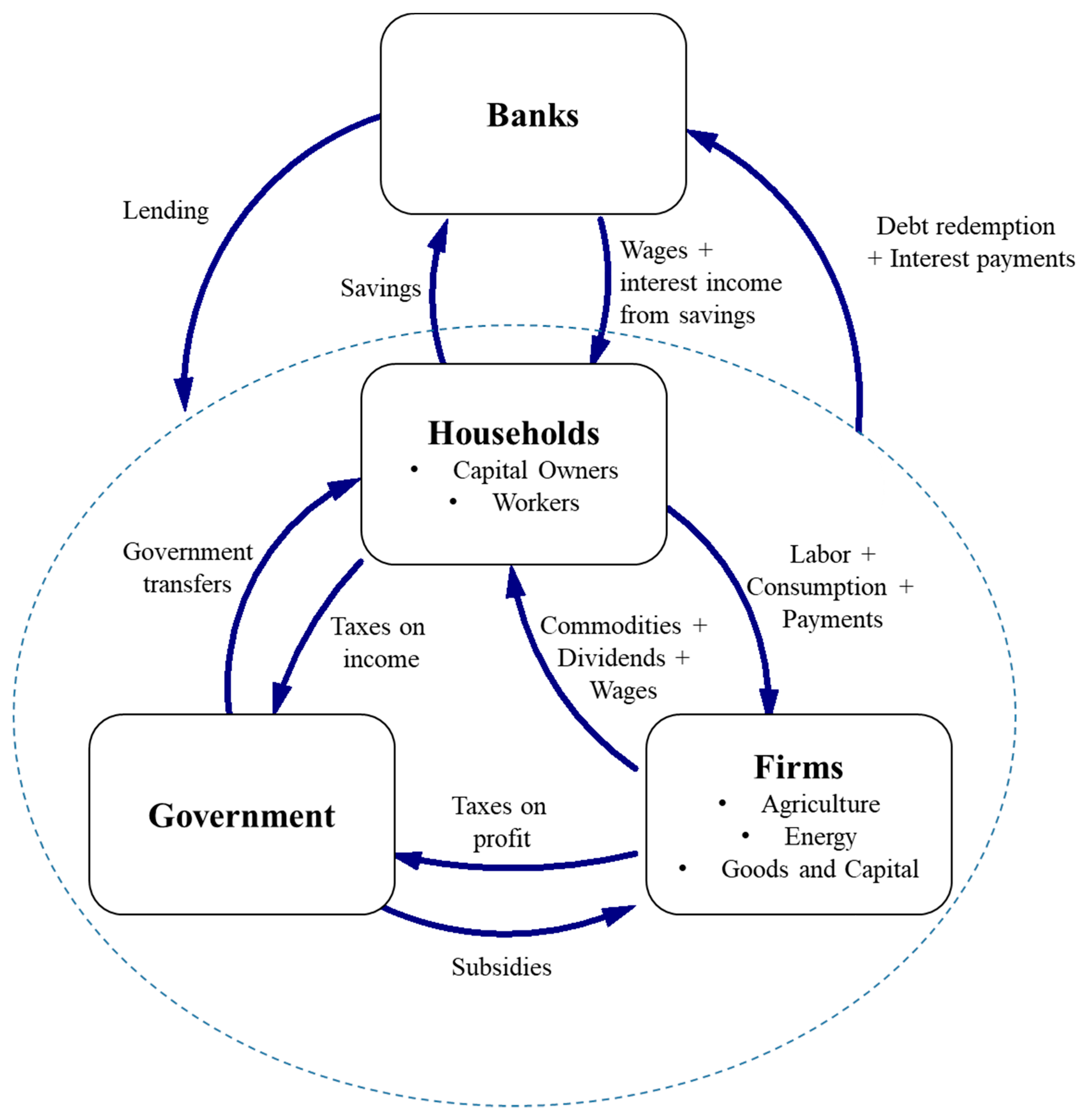
Figure 1 illustrates the overall relationships among the various sectors of the economy. Households lie at the core of the model, receiving cash flows from all other sectors, and they use those for consumption. Workers receive wages from firms and banks as a result of bank income from interest payments, and capital owners receive dividends from firms and interest payment income from banks that are allocated to depositors. In the model, only capital owners are assumed to have disposal income that allows money to be saved in banks. The fraction of capital owners to total population is assumed to be constant in the simulation. Households accumulate goods and capital as assets in their balance sheets, which, in turn, allows for a certain level of permissible debt calculated as a fraction of the former. In so doing, rising goods and capital purchase (because of population increases) rise households’ assets, which increase borrowing and, in turn, the accumulation of debt. The government collects taxes from both firms and households out of their profit and income and diverts those directly as inputs to households’ balance sheet as government transfers. This represents a simplification and indicates households as the ultimate beneficiary of all public services, infrastructures, and other expenditures of government. Besides this, the government can distribute subsidies to agriculture and energy sectors, and decide whether to finance those by reducing expenditure or rising public debt to the private sector.
While households increase their demand for each of the three productive sectors (EN, AC, and GC), firms perform investment decisions and hire workers to meet such a demand. The inventory (stock of output) is placed between consumption and production acting as a buffer to assure consumption can be met. The GC and EN share a similar structure in organizing input factors for production and are mostly based on the use of the Cobb-Douglas production function. The AC structure is taken from the World3 model [19]. All real stocks and flows related to physical trade have been reproduced as financial quantities and registered in their balance sheet. To finance their investments and costs of production, firms maintain a certain level of debt as a fraction of their assets dependent on their propensity to risk exposure. Based on their available cash, they face all costs of production—investments/depreciation of capital, investments in land development (only in the case of agriculture), payments for labor, payments for energy consumption, debt redemption, interest payments, and taxes—and distribute dividends. Interest rates, tax, and discard rates are fundamental components accounting for the cost of capital based on Hall and Jorgenson [44,45]. All costs of production (cost of capital, labor, energy) are reflected in the price of output of the commodity supplied by each sector, accounting for a delay representing the inability of firms to instantaneously measure and adapt prices to changes in costs. A mark-up is also taken into consideration, even though this is kept at zero in the case of cereal and energy because of the perfectly competitive markets they are assumed to operate into. The role of price in the model is of primary importance, considering it translates real to financial flows and vice-versa (Table 1).
In the model, price initialization of energy and the cereal commodities of the year 1995 have been based on the nominal value of the average price of coal, gas, and oil [46] and global food price of cereals [47].
Banks operate as money supply provider, as well as manage interest rates, to stabilize the economy at any point in time. In the model, the bank sector represents an aggregate of all financial transactions setting lending and borrowing at its core, including both private and central banks. In a very simplistic approach, the bank balance sheet is represented by cash, reserves, loans to the public, and loans to private sectors, whereas the liabilities are given by households’ deposits and a hypothetical stock of debt money. Such stock has particular importance, considering it represents the total amount of equity belonging to banking institutions that can be increased or decreased with the fiscal policy on the money supply.
The full economy described is stock and flow consistent. Table 2 shows the balance sheet matrix of the economy, with a sign (+) in front of every asset and a sign (−) in front of every liability.
In summary, the model provides a framework, which links together financial, human, and production systems, based on global energy reserves and land availability. Transactions are driven by real needs but governed by nominal flows. The government is assumed to facilitate the functioning of the overall system by providing subsidies to the agriculture and energy sectors. The financial system, which is based on household’s deposits, is assumed to generate money based on money demand and set the interest rate to assure stability in the economy.
3.1. Modeling the Financial Sector in the World3
World3 is a world model in which the financial and price systems have been made implicit in the relationships of the real economy. This was important to focus the model towards its purpose, that is to look at the dynamics of real output growth in a finite world by the year 2100. As a result, the model provides the foundations for the architecture of a global economy led by growth and capitalism, with very long-term dynamics. Feedback factors, including population dynamics and demographic transition, depletion of non-renewable resources over the century, accumulation of persistent and nonpersistent pollution that could ultimately reduce the life expectancy of the population, as well as destroy the agricultural system, are accounted for. Most importantly, an implicit industrial decision to prioritize agriculture above everything else when a polluted world lowers the productivity of land is a clear determinant for the collapse of the entire economic system.
In this paper, our purpose is to explore short-term dynamics between the price of food and energy, based on the volatility of the early 2000s. Such a purpose allows us to neglect long-term feedback systems, such as pollution, resource depletion, and demographic transitions. Different from the World3-03, variables, such as technology improvement potentials, that can impact the production of systems in the long-term are also neglected. Major sources of complexity in the model are included in the price modeling and variables, such as inventories and labor force.
3.2. The Agricultural Sector within the Economic Framework
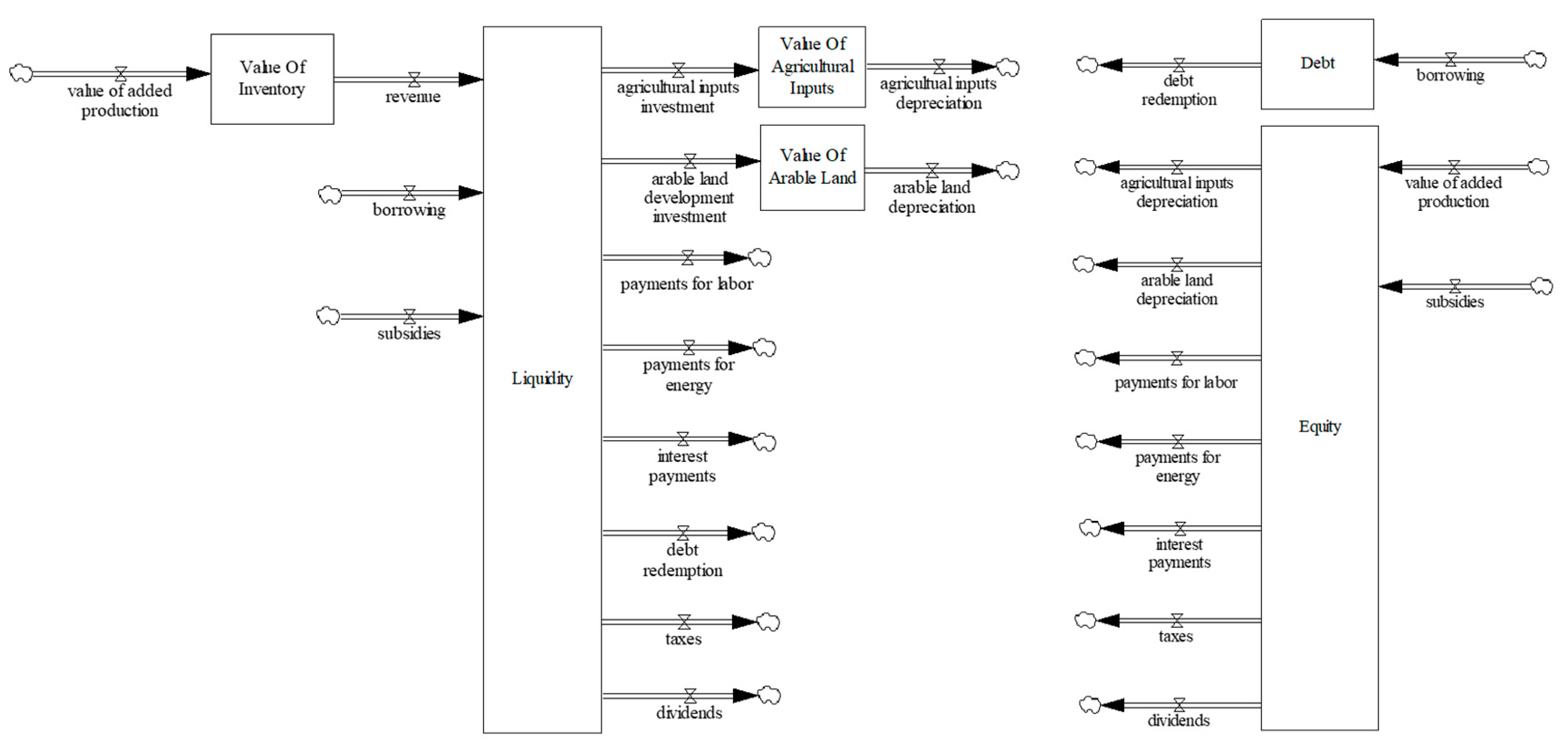
Figure 2 shows the balance sheet and cash flows of the agriculture sector. The left-hand side shows the financial assets in agriculture, whereas the right-hand side shows its liabilities. The equilibrium among the two sides is assured by recording every transaction on both sides, whereas the initial conditions are set by simply calculating the initial equity as the difference among the sum of the assets and the debt. It is worth noting that the physical assets on the assets side are shared between equity and debt on the liabilities side.
The cash flows out of the stock ‘Liquidity’ are all calculated based on different rules and follow different dynamics. However, each of them is also influenced by a non-linear correction factor dependent on the availability of cash in the ‘Liquidity’ stock itself. In the extreme case, where the inflows of cash in ‘Liquidity’ would switch off, the liquidity would quickly reduce to zero because of continuous outflows of payments. To increase realism in the model, the liquidity stock is not allowed to go below zero, and non-linear relationships that bring outflows to zero while liquidity approaches zero are fundamental. In the case of excess liquidity, several payments would remain the same as the one indicated by further calculations (i.e., taxes, interest payments, payments for energy), indicating that money surpluses would not alter those. Other payments can be increased to assure the cash is well used in the time of growth, including Capital Investments, Payments for Labor, Debt Redemption, and Dividends.
The equations that are most relevant for the presentation of this study are the ones that relate to trade with the other sectors. In particular, the main inflow to the stock of Liquidity is the revenue () of the agriculture sector, which is determined by the price of agricultural output () and the cereal consumption form households (), as indicated in Equation (1).
Particular importance is given to the equations describing the investments in new assets, which have been adapted from the World3-03 model. In particular, all capital units of the World3 model have been converted into GC units for our model. This allowed the introduction of the price of the GC unit (pc), which is used as a multiplier of the W3 agricultural inputs quantities to obtain financial flows and stocks of assets.
Despite the use of the World3 model structure for generating food output production, the structure adapted to connect its investment function with our model is the inverse in reasoning. In particular, the investment allocation in the agricultural sector of the World3 divides a total amount of agricultural investment into smaller parts that are allocated between agricultural inputs and land development. To do so, a fraction of agricultural inputs allocated to land development () is first calculated based on the marginal productivity of both agricultural inputs and arable land and then used to split the total agricultural investments between the two [44]. In our model, instead, we first calculate agricultural inputs investment () and use this as a driver for the investment in arable land development (). In particular, the investments in agricultural inputs (AII) have been first translated into real quantities (), divided by a factor () to obtain the amount of total agricultural investments as used in World3, and then multiplied again by to obtain the real investment in land development. This is, then, multiplied by the price of capital () to obtain financial flows to include in the balance sheet, as shown in Equation (2).
The total amount of indicated energy consumed is based on the agricultural inputs ( —i.e., indicating the number of chemicals and equipment in use in agriculture), and calculated as a simple multiplication between and their energy intensity (). Payments for energy () within the agriculture sector are then dependent on the price of energy (). However, a non-linear relationship dependent on the availability of liquidity () is also applied to account for decreases in affordability of energy consumption when cash is constrained. In turn, this limit constrains energy demand from agriculture and the revenue in the energy sector. Equation (3) describes this behavior.
The variations in the prices of commodities have the important effect of generating economic instability, which drives changes in the money supply, inflation, and investments decision allocation. The stability of the system is delegated to the banking system, responsible for both money creation and managing interest rates. Such a structure has been taken from Sterman [20]. While affected by the price change, the interest rate impacts the cash flows of the various sectors, as described in Equation (4). The desired interest payment is calculated as a multiplication between the interest rate () and debt (), and such a value is corrected with a non-linear relationship responsible for controlling cash flows in case of deficit or surplus of liquidity according to required levels.
Similar reasoning is given to the payments of labor (which is a multiplication between wages and employed people corrected with non-linearity) and debt redemption (which is assumed to be a constant fraction of debt based on the average duration of a loan and corrected with a non-linear relationship). The profit before tax is then calculated as a difference between revenue, cost of production (i.e., payments for energy and labor), and cost of physical assets (debt redemption, interest payments, agricultural inputs, and land depreciation). Taxes are applied as a multiplication of such a quantity and a constant tax rate. The profit after tax is then calculated, which drives the distribution of dividends to the capital owners. Without the presence of subsidies, the sector tends to recreate a cash-flow balance between inputs and outputs from the stock liquidity by generating borrowing, which increases the stock of debt.
Figure 3 shows the price of output at the center of the feedback loop structure of the agricultural system of our model, showing the interplay of major elements and forces determining its behavior. The driving force, generating growth in the model, is given by population (exogenous in the model based on UN data). At the real and natural levels, the agricultural sector dynamics of land-use change and investments allocation among agricultural inputs and land development follow World3 [19,22,38].
The major feedback loops involving price within the agricultural system are represented in Figure 3. While reinforcing feedback loops (R1, R2, and R3) tend to destabilize the system towards disequilibrium, the balancing loops (B1, B2) generate the forces that assure supply is in line with demand. The reinforcing feedback loops describe the positive market forces that support a functioning economic system. In particular, R1 indicates that increases in demand (driven by population growth) correspond to increases in consumption and, in turn, revenue. The higher the revenue, the greater the profit and, in turn, dividends. Price increases tend to be self-reinforcing through the feedback loops R2 and R3. In particular, price increases are assumed to drive inflation, which implies further price increases. At the same time, inflation generates increases in wage, which raises the cost of production (it is worth noting that the cost of labor is the larger share for the cost of production in the model), and thus increases prices accordingly.
The continuous rise in the price of output strengthens the market forces that are responsible for balancing the system and bringing the supply to match the demand. In particular, B2 recreates the behavior of farmers who will tend to produce more when the prices are higher as they look for increased profits and revenues. An effect of price change is introduced in determining investments, which, in turn, raises the availability of arable land and agricultural inputs that, in turn, increase production and the inventory. The higher those values, the stronger the feedback to balance prices towards dynamic equilibrium levels. At the same time, increases in demand, in turn, increases investments, productive assets, and thus production (B1). It is worth noting that, by building on the World3 structure, labor and energy have been modeled as driven by the agricultural inputs with a simple corrective factor. In so doing, costs of labor and energy (and the demand of energy to EN) tend to rise proportionally with the increases in agricultural inputs (which is manufactured from the GC sector).
Subsidies are assumed to be a constant fraction of government expenditures allocated as a monetary input to the agricultural sector cash stock. Such allocation can be modeled in different ways according to the user’s need. Subsidies can be financed through borrowing, such as increasing government debt and maintaining their same level of expenditure, or gradually by deducing some expenditure, which, in turn, decreases cash availability for households’ consumption. In the base run of the model, we use the former. Figure 4 shows the use of subsidies in the agriculture sector. The most important feedback generated by subsidies is to balance the price.
By reducing the cost of production, subsidies reduce price, which, in turn, reduces revenue (B3). Also, our model includes subsidies as direct determinants in the reduction of price to maintain a more affordable price level for households (B4). In the base run scenario of the model, one fraction is normally paid as subsidies in agriculture and another fraction in energy (i.e., 1% of government’s revenues in agriculture, and 8% of government’s revenue in energy). Such values can be tested to see whether and how subsidies to the agricultural and energy sectors can affect food price change over time.
3.3. Energy, Food, and Inflation
The purpose of the ETE model was to look at the possible implications for energy shortages on inflation in the US economy [20]. As a result, the important emphasis was given to the modeling of a GDP Deflator, as well as the trend in prices that could lead to a measure for inflation in the model.
In the current model, we extend that structure by exploring the effects of closing the feedback from inflation (calculated as the average variations of prices in the goods and capital and food sector) and the direct input to the inflation of every price calculation. Such feedback can be considered as a potential short-term mechanism of traders, exploiting a reinforcing feedback loop in speculating higher prices when prices start to increase.
Figure 5 shows the causal loop diagram for the modeling of the prices in the energy sector that remains at the core of the entire economic system. In a closed-loop economy, energy prices increase the cost of production of every commodity in the economy. This involves both the energy itself and in the case of this model, agricultural and capital commodities. The reinforcing feedback that increases the price further is two-fold. On the one hand, the increase in cost determines a tendency to raise the price of energy (R1). On the other hand, the cost of energy raises the prices of the other commodities that, in turn, impacts overall inflation and finally can increase the price of energy (R2). In addition to those important feedbacks, the supply and demand of each commodity play a key role to balance the price. Given the inclusion of inventory factors, the supply-demand effect is calculated as the sum of the ratios of production and inventory levels with relative elasticities.
4. Introducing Shocks
The model is a closed dynamic economy which aggregates all cereal, energy, and other commodities production as if they are global aggregates. In so doing, the economy tends to run smoothly in a four macro-agents’ (food, energy, goods and capital, and households) economic system driven by a supply/demand network in which each sector is responsible for providing a particular commodity required by the others. As a result, the model represents the economy with a very simplified set of equations. Thus, the model is not supposed to capture shocks and policy change in its endogenous structure by construction. The shocks have to be exogenously introduced, simulating a hypothetical uncontrollable effect emerging from the reality of the system under study, but still not yet understood. In this sense, the strength of the model is not in the prediction of global shocks but the analysis of cascade effect of such shocks on the rest of the system, characterized by complex feedback loops, accumulation processes, and non-linear behaviors. Over time, the model could be expanded to capture significant factors explaining social behaviors, including political unrest and impact of institutions.
Depicting real-world dynamics, prices lie at the core of the dynamics of the model, governing supply-demands, revenue streams, and have the power to strongly affect investments in each sector that drive production change. Besides, the role of inflation particularly complicates the analysis. The weighted average of price changes based on the production pattern for each commodity is assumed to contribute to overall inflation (GDP deflator measure). Perceived inflation provides feedback to the price change of each commodity directly (increase in price) and indirectly through costs of production that drive the price in the model (on the one hand, by increasing wages, and on the other hand, as production costs due to other commodity prices change). The complete model accounts for approximately 60 stock variables, 100 parameters, and 400 auxiliary variables. The purpose of the model is to capture a part of the complex relationship between food and energy prices via two main feedback loops. First, a feedback from the energy to food via the cost of production increase, and secondly, feedback from food to energy via possible impact on inflation behaviors that can impact back on the setting of the energy price.
In the short-term, a price spike of a particular commodity increases the overall value of production, the cash into the sector responsible for producing such a commodity, and, in turn, increases profits and income for households from that commodity. The rise in revenue for the firm sector allows for increasing investments for higher production. With a delay, demand drops, production rises above demand, and prices oscillate to lower levels. In the longer time frame (a few years), prices will tend to stabilize again to initial levels. Within this context, the energy price dynamics have particular importance in the study because they drive the production cost change in all sectors. Food prices instead impact on the overall consumption level of households, who allocate a share of their income to meet their nutritional needs.
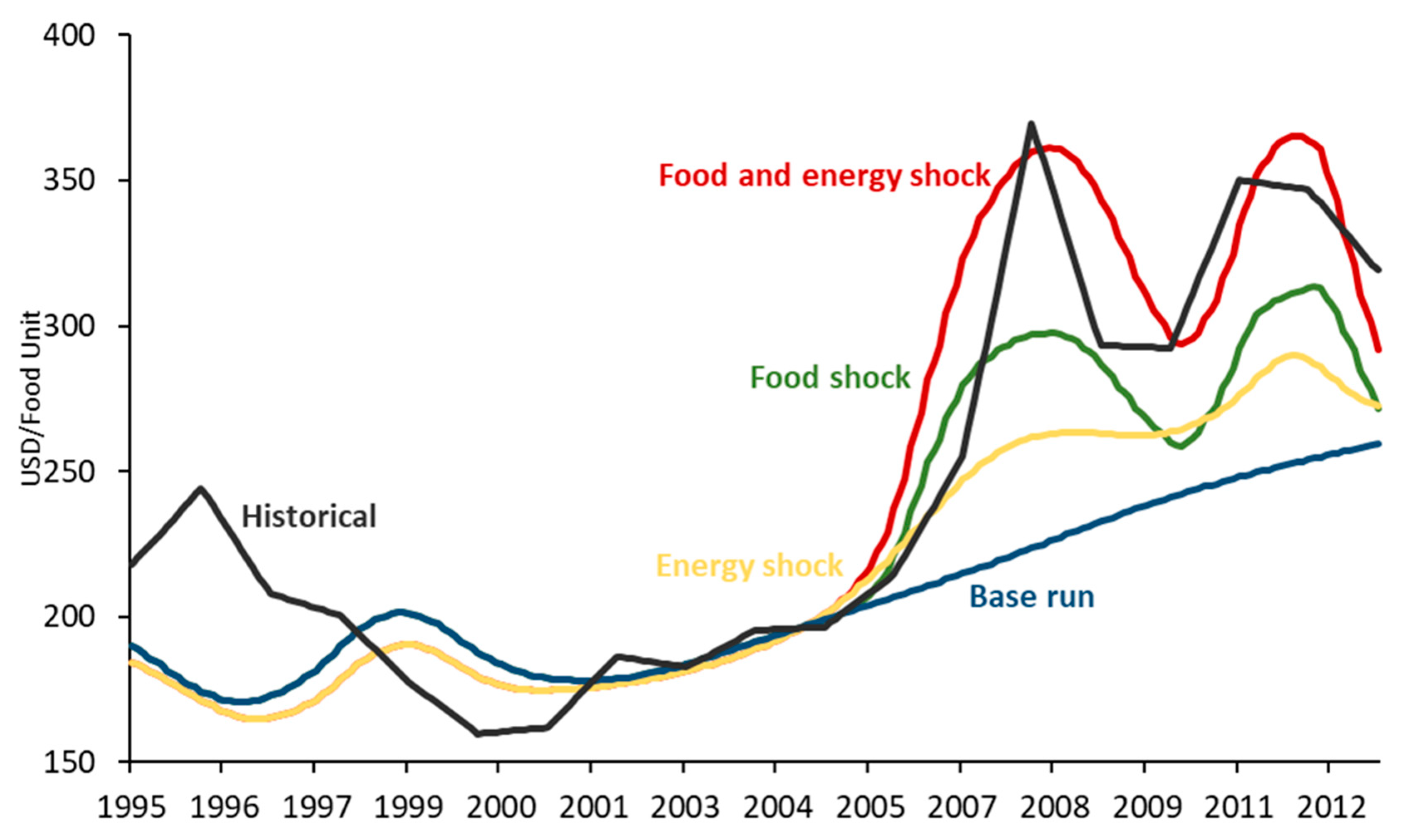
We generate five shocks to run four different scenarios to attempt to reproduce historical data on food and energy price change, as depicted in Figure 6 and Figure 7. The historical time series chosen is between 1995 and 2013 as it contains both a period of relative stability in both food and energy prices, as well as significant shocks (2004–onwards). Therefore, we attempt to reproduce these historic shocks in prices by applying exogenous shocks in production, prices, or subsidies. A direct price shock acts as a proxy for speculative behavior from financial markets, where the underlying physical or subsidy constraints cannot solely account for the actual price shock observed. If our model allows us to reproduce those historic price shocks, then it could be used to test the susceptibility of our future food and energy systems to similar shocks, as well as test potential policy responses that may help reduce the scale of these price shocks.
Shocks in the model can be applied to both energy and food sectors as (i) constraint on the supply (production shocks), (ii) direct effect on price change (price shocks), and (iii) change in government’s subsidies to allocate government revenues on sector’s liquidity. The scenarios proposed are:
- Base run (blue line in Figure 6 and Figure 7)—represents the natural dynamic of the system as it was built. In this sense, the food and energy production shocks remain at zero for the full duration of the simulation. Subsidies in energy correspond to 5% of government income for the full duration of the simulation.
From the scenario runs, it is clear to see that the base run (blue) produces a relatively stable price for energy and food over the period under consideration. This is as expected. We use the shocks seen in real energy prices (Figure 6) and real food prices (Figure 7) after 2007 to calibrate our scenarios. The size of the scenario shocks is, therefore, derived from matching the historic price data to the model price data.
What emerges from this analysis is that both food and energy price shocks tend to affect the price of another commodity non-linearly. Looking at the difference between the base run and the food shock scenarios in both figures, it is possible to see how those inputs affect the price of food. It is interesting to note that a food shock also creates an energy price shock. This is due to both the influence of food on inflation that affects the energy pricing and to the fact that when some food production is destroyed, additional production is necessary for years to come to stabilize production levels towards demand satisfaction. This requires additional energy, which corresponds to an increase in energy demand, and this drives energy price change in the short-term. However, a much stronger relationship exists in the opposite direction with an energy shock, resulting in a stronger food price shock.
The result of including both food and energy shocks simultaneously in the model replicates, with higher fidelity, the final shape of the food and energy prices, as found in the Food and Agriculture Organization Corporate Statistical Database (FAOSTAT) [47] and World Bank Global Economic Monitor (WB GEM) Commodities [46] datasets accordingly. The most interesting result of this analysis is that the sum of the shocks does not correspond to a summed effect on the price change. Due to the time lags, path dependency, and feedback loop structure, both effects of food and energy prices results are amplified when accounted for together in comparison to the food and energy shocks affecting the system alone.
We note that the two peaks seen in the energy and food prices around 2008 and 2011 can be captured using our dynamic model. In particular, to recreate the observed price shocks, we need a joint food and energy production shock between 2003 and 2006, price shocks in both energy and food around 2010–2011 (a proxy for market speculation), and a decrease in government subsidies to energy over that period. The production shock in food could be due to the loss of agricultural output due to extreme weather in a key breadbasket (for example, drought or floods in China or the USA), while a production shock in energy could be due to geopolitical factors as much as physical factors (for example, trade restrictions or unrest in key energy-producing regions). Other options could consider the high growth rate in energy demand concentrated in countries, such as China, which could also cause the speculative price shocks. Further work and model structures would be necessary to capture more complex theories on the analysis of historical data.
There is evidence of these underlying shocks all occurring over that period [48], albeit not at the exact levels that we use in our scenarios. We note, as above, that the food price shock observed is likely caused by both a shock in the food and energy systems, whereas the energy price shock is more driven by the energy system alone. We also note that while it may be possible to reproduce the historic data with a different combination of exact values in those underlying shocks, we found it very difficult to reproduce the exact features by only shocking one aspect (either production, price, or subsidy) without those shocks appearing unreasonable.
Further work is needed to explore whether the size of the shocks used in the scenarios reflects accurately the real physical or financial shocks (or a combination of these) or if other market behaviors (such as financial futures markets over-pricing shocks) could account for some of the increases in prices. We note that it is likely that the actual size of these shocks is likely to be too high, given market responses (which tend to amplify the impacts of shocks) are not captured in our model. In particular, we note that there is also an important aspect of where subsidies are applied as a dramatic local change in food, or energy subsidies may not have a consequent impact on global subsidies (may not be seen as a global shock in subsidies) but could have a much larger impact on global food prices depending on exactly when, where, and how the subsidies are changed.
This analysis offers a very useful tool to explore the physical and financial size of a shock required to produce a market-based price response, as seen in the historic data.
5. Conclusions
By building on the structure of the Limits to Growth World3 model [19], the Money and Macroeconomy Dynamics (MMD) [21], and the Energy Transition and the Economy model [20], we present a novel integrated global food and energy security systems dynamics model. We use the model to assess the conditions for the onset of systemic risk emerging from the interaction between natural resources, real, and financial system dimensions at the global level as a consequence of exogenous shocks.
Then, we show how system dynamics can provide a platform for supporting ‘what if’ behavioral scenario analysis to study the socio-economic impact of systemic and cascading risks, and the role (and trade-offs) of alternative responses to policies, with a focus on global food security. Production and consumption goods firms of the economy are represented in their linkages with the agricultural sector, in terms of economic and financial accounting. Moreover, the important linkage with the government sector, which is responsible for providing subsidies to the energy and agricultural sectors, is included. This is fundamental to analyze the impact of public policies on a system’s resilience to shocks impacting the food system.
The model dynamics are centered on the role of prices, which are endogenously modeled in the system and represent leverage points for destabilizing the system at both the real and financial levels of the economy. A base run scenario is simulated, calibrating the model on the historical data of crops and fossil fuels resource prices. Multiple price spikes, as well as production shocks and changes in the level of subsidies, are then added to the reference run with the key objective of replicating the historical observed volatility in resource prices. Our results show that the energy system has a more significant impact on the food system than vice versa in channeling and responding to the shocks. This has important implications when designing policies to address future volatility in both energy and food markets. In particular, when considering the design of global food aid responses to potential shocks, it is important for policymakers to consider as much the underlying energy system, and its instabilities, as it is for them to consider the food system. This points to the need for a much more holistic approach to designing interventions in risk management. Additionally, we could not reproduce the past shocks without using a complex and likely interconnected combination of underlying drivers, including shocks in production, market responses (through prices), and government support (through subsidy).
Such a model structure is not able, by design, to endogenously generate shock dynamics, like the example provided in Section 3 shows. However, it allows the analysis of shocks scenarios, in terms of drivers of the system’s responses, to identify the conditions for reinforcing feedback loops to emerge, and their impact on the system’s stability. By taking into account the role of financial, real, and natural capital and investments, the model is a step forward towards an integrated assessment tool that can be used to test alternative scenarios driven by uncertainty and risk, such as climate extreme events and their impacts on food production, returning decision-makers accessible timely information for building resilience.
This model aims to contribute to the development of alternative storytelling scenarios to simulate the impact of climate risk on interconnected human-environmental systems, and the role of public policies as drivers of resilience in the short-term.
Author Contributions
Conceptualization, R.P. and A.J.; methodology, R.P. and I.M.; software, R.P.; formal analysis, R.P.; writing—original draft preparation, R.P.; writing—review and editing, A.J. and I.M.; supervision, I.M and A.J.; funding acquisition, A.J.
Funding
This research was funded by the Dawe Charitable Trust and the Economic and Social Research Council for the Center for the Understanding of Sustainable Prosperity (CUSP) (ESRC grant no: ES/M010163/1).
Acknowledgments
The authors would like to thank the three anonymous reviewers of an earlier version of this paper that was presented at a conference for their valuable comments, which have strengthened the structure and presentation of results. The authors would also like to thank the three anonymous reviewers of this final paper.
Conflicts of Interest
The authors declare no conflict of interest. The funders had no role in the design of the study; in the collection, analyses, or interpretation of data; in the writing of the manuscript, or in the decision to publish the results.
References
- IPCC. Climate Change 2014: Impacts, Adaptation, and Vulnerability, Summary for Policymakers; Cambridge University Press: Cambridge, UK; IPCC: New York, NY, USA, 2014. [Google Scholar]
- Munich Re. Group Annual Report 2013. 2013. Available online: www.munichre.com (accessed on 1 August 2018).
- ADB. ADB Annual Report 2013. 2013. Available online: http://www.adb.org/documents/adb-annual-report-2013 (accessed on 1 August 2018).
- Jones, A.; Hiller, B. Exploring the dynamics of responses to agrifood production shocks. Sustainability 2017, 9, 960. [Google Scholar] [CrossRef]
- Godfray, H.C.; Beddington, J.R.; Crute, I.R.; Haddad, L.; Lawrence, D.; Muir, J.F.; Pretty, J.; Robinson, S.; Thomas, S.M.; Toulmin, C. Food security: The challenge of feeding 9 billion people. Science 2010, 327, 812–818. [Google Scholar] [CrossRef] [PubMed]
- WRI. Creating a Sustainable Food Future—A Menu of Solutions for Sustainability Feed More Than 9 Billion People by 2050. 2014. Available online: www.wri.org/sites/default/files/wri13_report_4c_wrr_online.pdf (accessed on 1 August 2018).
- IFPRI. Global Hunger Index—The Challenge of Hunger: Focus on Financial Crisis and Gender Inequality. 2009. Available online: cdm15738.contentdm.oclc.org/utils/getfile/collection/p15738coll2/id/15025/filename/15026.pdf (accessed on 1 August 2018).
- IPCC. 5th Assessment Report. Summary for Policy Makers. In Climate Change 2013: The Physical Science Basis; Contribution of Working Group I to the Fifth Assessment Report of the Intergovernmental Panel on Climate Change; IPCC: Geneva, Switzerland, 2013. [Google Scholar]
- Benton, T.; Bailey, R.; Challinor, A.; Elliott, J.; Gustafson, D.; Hiller, B.; Jones, A.; Jahn, M.; Kent, C.; Lewis, K. Extreme Weather and Resilience of the Global Food System; Final Project Report from the UK-US Taskforce on Extreme Weather and Global Food System Resilience; The Global Food Security Programme: Swindon, UK, 2015. [Google Scholar]
- Puma, M.J.; Bose, S.; Chon, Y.; Cook, B. Assessing the evolving fragility of the global food system. Environ. Res. Lett. 2015, 10. [Google Scholar] [CrossRef]
- Natalini, D.; Jones, A.W.; Bravo, G. Quantitative assessment of political fragility indices and food prices as indicators of food riots in countries. Sustainability 2015, 7, 4360–4385. [Google Scholar] [CrossRef]
- Abbott, P.C.; Hurt, W.E.; Tyner, C. What’s driving food prices? Farm Foundation Issue Report. 2008. Available online: www.farmfoundation.org/webcontent/Farm-Foundation-Issue- Report-Whats-Driving-Food-Prices-404.aspx?z=na&a=404 (accessed on 1 August 2018).
- Diao, X.; Headey, D.; Johnson, M. Toward a green revolution in Africa: What would it achieve, and what would it require? Agric. Econ. 2008, 39, 539–550. [Google Scholar] [CrossRef]
- Mitchell, D. A Note on Rising Food Prices; World Bank Policy Research Working Paper 4682; World Bank: Washington, DC, USA, 2008. [Google Scholar]
- Lloyd’s of London, Food system shock—The Insurance Impacts of Acute Disruption to Global Food Supply. 2015. Available online: https://www.lloyds.com/~/media/files/news%20and%20insight/risk%20insight/2015/food%20system%20shock/food%20system%20shock_june%202015.pdf (accessed on 1 August 2018).
- Baumeister, C.; Kilian, L. Do Oil Price Increases Cause Higher Food Prices? Econ. Policy 2014, 29, 691–747. [Google Scholar] [CrossRef]
- Balcombe, K.; Rapsomanikis, G. Bayesian estimation of nonlinear vector error correction models: The case of sugar-ethanol-oil nexus in Brazil. Am. J. Agric. Econ. 2008, 90, 658–668. [Google Scholar] [CrossRef]
- Qiu, C.; Colson, G.; Escalante, C.; Wetzstein, M. Considering macroeconomic indicators in the food before fuel nexus. Energy Econ. 2012, 34, 2021–2028. [Google Scholar] [CrossRef]
- Meadows, D.; Randers, J.; Meadows, D. Limits to Growth: The 30-Year Update; Chelsea Green Publishing: Hartford, VT, USA, 2003. [Google Scholar]
- Sterman, J.D. The Energy Transition and the Economy: A System Dynamics Approach. Ph.D. Thesis, Massachusetts Institute of Technology, Cambridge, MA, USA, 1981. [Google Scholar]
- Yamaguchi, K. Money and Macroeconomic Dynamics-Accounting System Dynamics Approach. 2013. Available online: http://www.muratopia.org (accessed on 1 July 2017).
- Meadows, D.L.; Behrens, W.W.; Meadows, D.L.; Naill, R.F.; Randers, J.; Zahn, E.K.O. The Dynamics of Growth in a Finite World; Wright-Allen Press: Cambridge, MA, USA, 1974. [Google Scholar]
- Gerasimchuk, I.; Bassi, A.M.; Ordonez, C.D.; Doukas, A.; Merrill, L.; Whitley, S. Zombie Energy: Climate Benefits of Ending Subsidies to Fossil Fuel Production; Global Subsidies Initiative: Geneva, Switzerland, 2017. [Google Scholar]
- Bast, E.; Makhijani, S.; Pickard, S.; Whitley, S. Fossil Fuel Bailout: G20 Subsidies to Oil, Gas and Coal Exploration; Overseas Development Institute/Oil Change International: London, UK; Washington, DC, USA, 2014; Available online: http://priceofoil.org/content/uploads/2014/11/G20-Fossil-Fuel-Bailout-Full.pdf (accessed on 22 July 2019).
- Coady, D.; Parry, I.; Sears, L.; Shang, B. How Large are Global Energy Subsidies? (IMF Working Paper WP/15/105). 2015. Available online: https://www.imf.org/external/pubs/ft/wp/2015/wp15105.pdf (accessed on 22 July 2019).
- Selvaraju, R. Climate risk assessment and management in agriculture. Building resilience for adaptation to climate change in the agriculture sector. In Proceedings of the Joint FAO/OECD Workshop, Rome, Italy, 23–24 April 2012; p. 71. [Google Scholar]
- Müller, C.; Robertson, R.D. Projecting future crop productivity for global economic modeling. Agric. Econom. 2014, 45, 37–50. [Google Scholar] [CrossRef]
- Rosenzweig, C.; Elliott, J.; Deryng, D.; Ruane, A.C.; Müller, C.; Arneth, A.; Boote, K.J.; Folberth, C.; Glotter, M.; Khabarov, N.; et al. Assessing agricultural risks of climate change in the 21st century in a global gridded crop model intercomparison. Proc. Natl. Acad. Sci. USA 2014, 111, 3268–3273. [Google Scholar] [CrossRef] [PubMed]
- Monasterolo, I.; Janetos, A. Exploring opportunities for integration of alternative modeling approaches for the analysis of climate change impacts on agriculture. Presented at the 8th IAMC conference, Potsdam, Germany, 15–18 November 2015. [Google Scholar]
- Frank, S.; Witzke, H.P.; Zimmermann, A.; Havlík, P.; Ciaian, P. Climate change impacts on European agriculture: A multi model perspective. In Proceedings of the XIVth EAAE Congress “Agri-Food and Rural Innovations for Healthier Societies”, Ljubbljana, Slovenia, 26 August 2014. [Google Scholar]
- Forrester, J.W. Industrial Dynamics; MIT Press: Cambridge, MA, USA; Wiley: New York, NY, USA, 1961. [Google Scholar]
- Sterman, J.D. Business Dynamics: Systems Thinking and Modeling for a Complex World; Irwin/McGraw-Hill: New York, NY, USA, 2000. [Google Scholar]
- Forrester, J.W.; Senge, P.M. Tests for building confidence in system dynamics models. In System Dynamics; Legasto, A.A., Forrester, J.W., Lyneis, J.M., Eds.; North-Holland: Amsterdam, The Netherlands, 1980. [Google Scholar]
- Morecroft, J.D.W. System dynamics and microworlds for policymakers. Eur. J. Operat. Res. 1988, 59, 9–27. [Google Scholar] [CrossRef]
- Meadows, D.H.; Meadows, D.L.; Randers, J.; Behrens, W.W. The Limits to Growth; Universe Books: New York, NY, USA, 1972; p. 102. [Google Scholar]
- Forrester, J.W. World Dynamics; Wright-Allen Press: Cambridge, MA, USA, 1971. [Google Scholar]
- Monasterolo, I.; Pasqualino, R.; Mollona, E. The role of system dynamics modelling to understand food chain complexity and address challenges for sustainability policies. In Proceedings of the 1st FAO-SYDIC Conference, Rome, Italy, 6–7 July 2015. [Google Scholar]
- Meadows, D.H.; Meadows, D.L.; Randers, J. Beyond the Limits: Confronting Global Collapse Envisioning a Sustainable Future; Chelsea Green Pub Co.: Hartford, VT, USA, 1992. [Google Scholar]
- Rockström, J.; Steffen, W.; Noone, K.; Persson, Å.; Chapin, F.S., II; Lambin, E.; Lenton, T.M.; Scheffer, M.; Folke, C.; Schellnhuber, H.; et al. Planetary boundaries: Exploring the safe operating space for humanity. Nature 2009, 461, 472–475. [Google Scholar]
- Jones, A.; Allen, I.; Silver, N.; Cameron, C.; Howarth, C.; Caldecott, B. Research report—Resource constraints: Sharing a finite world. Implications of Limits to Growth for the Actuarial Profession. 2013. Available online: www.actuaries.org.uk (accessed on 22 July 2019).
- Randers, J. From limits to growth to sustainable development or SD (sustainable development) in a SD (system dynamics) perspective. Syst. Dyn. Rev. 2000, 16, 213–224. [Google Scholar] [CrossRef]
- Randers, J. 2052: A Global Forecast for the Next Forty Years; Chelsey Green: Post Mills, VT, USA, 2012. [Google Scholar]
- Pasqualino, R.; Jones, A.W.; Monasterolo, I.; Phillips, A. Understanding global systems today—A calibration of the World3-03 model between 1995 and 2012. Sustainability 2015, 7, 9864–9889. [Google Scholar] [CrossRef]
- Hall, R.E.; Jorgenson, D.W. Tax policy and investment behavior. Am. Econ. Rev. 1967, 57, 391–414. [Google Scholar]
- Hall, R.E.; Jorgenson, D.W. Tax policy and investment behavior: Reply and further results. Am. Econ. Rev. 1969, 65, 388–401. [Google Scholar]
- World Bank Global Economic Monitor (GEM) Commodities. 2015. Available online: http://databank.worldbank.org/data/reports.aspx?source=Global-Economic-Monitor-%28GEM%29-Commodities (accessed on 1 August 2018).
- FAOSTAT. 2015. Available online: http://faostat3.fao.org/home/E (accessed on 1 August 2018).
- Jones, A.; Phillips, A. Historic food production shocks: Quantifying the extremes. Sustainability 2016, 8, 427. [Google Scholar] [CrossRef]
Figure 1.
Major flows and sectors in the model.

Figure 2.
Financial statement in the agricultural sector.

Figure 3.
Causal loop diagram of the agricultural sector connecting real and financial variables and completely based on the dynamics of price.
Figure 3.
Causal loop diagram of the agricultural sector connecting real and financial variables and completely based on the dynamics of price.
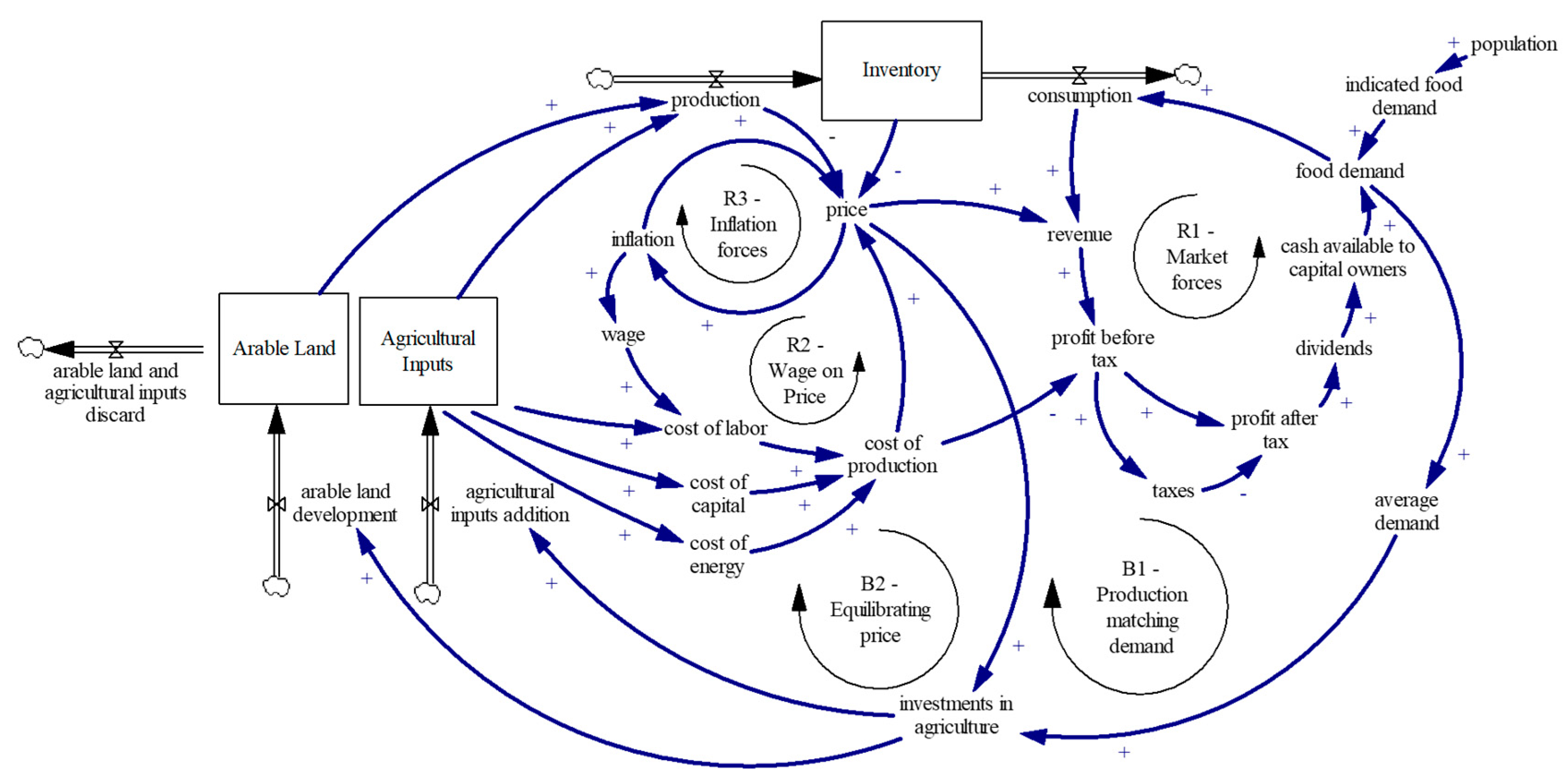
Figure 4.
Causal loop diagram of the effect of government taxes and subsidies on agriculture finances.
Figure 4.
Causal loop diagram of the effect of government taxes and subsidies on agriculture finances.
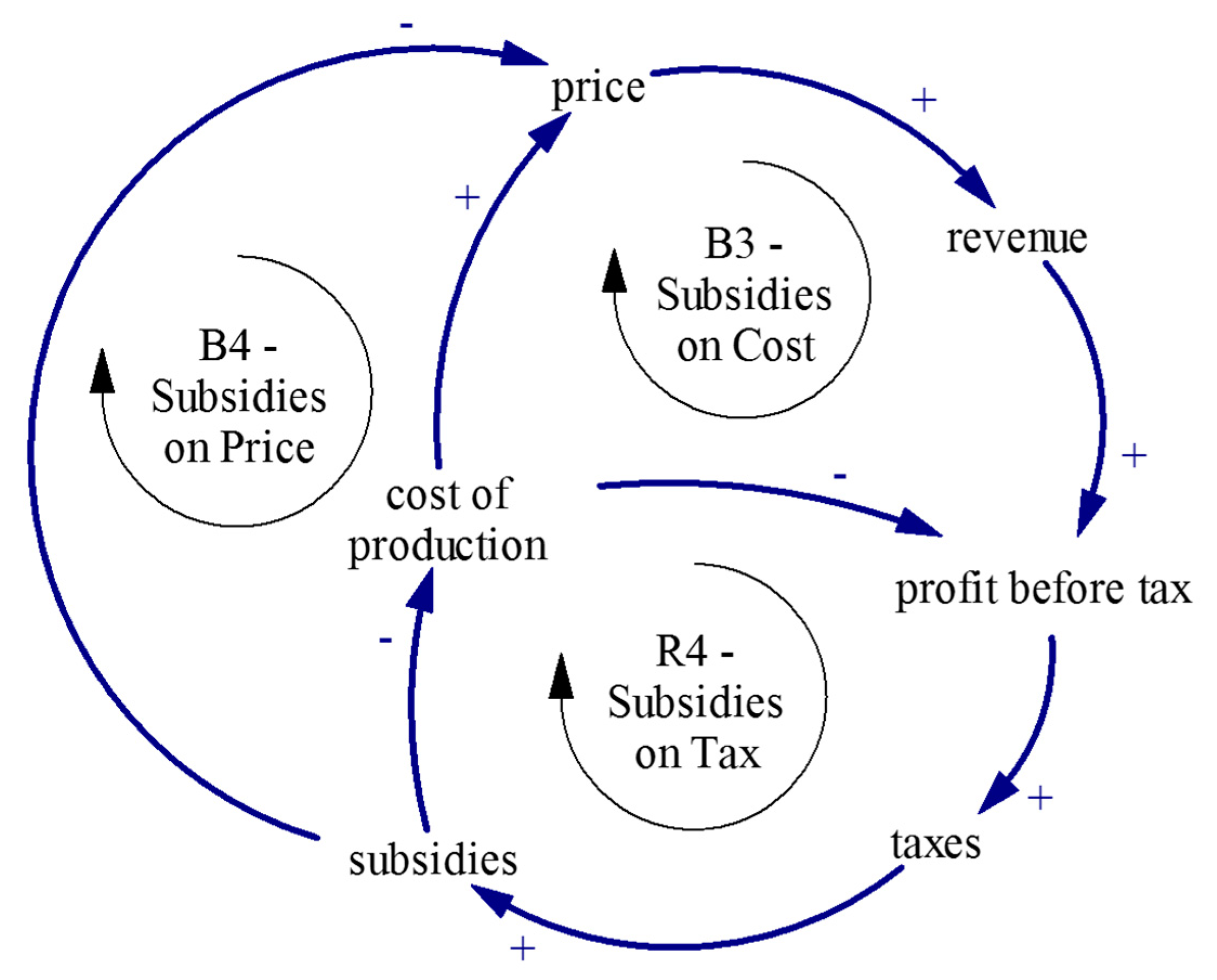
Figure 5.
Causal loop diagram of the effect of energy price as a foundation to the rest of the economy.
Figure 5.
Causal loop diagram of the effect of energy price as a foundation to the rest of the economy.
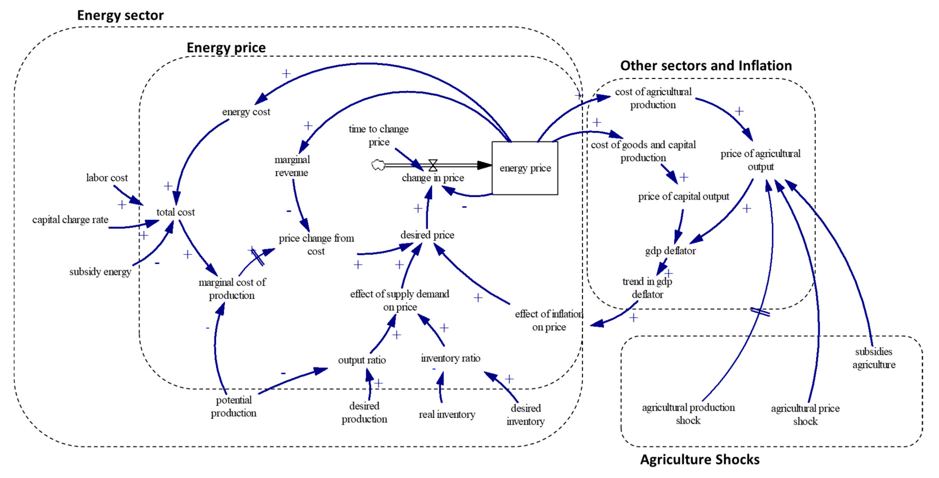
Figure 6.
Energy historic price data (own elaboration from [46]) compared to the base run scenario and shock scenarios of the model.
Figure 6.
Energy historic price data (own elaboration from [46]) compared to the base run scenario and shock scenarios of the model.
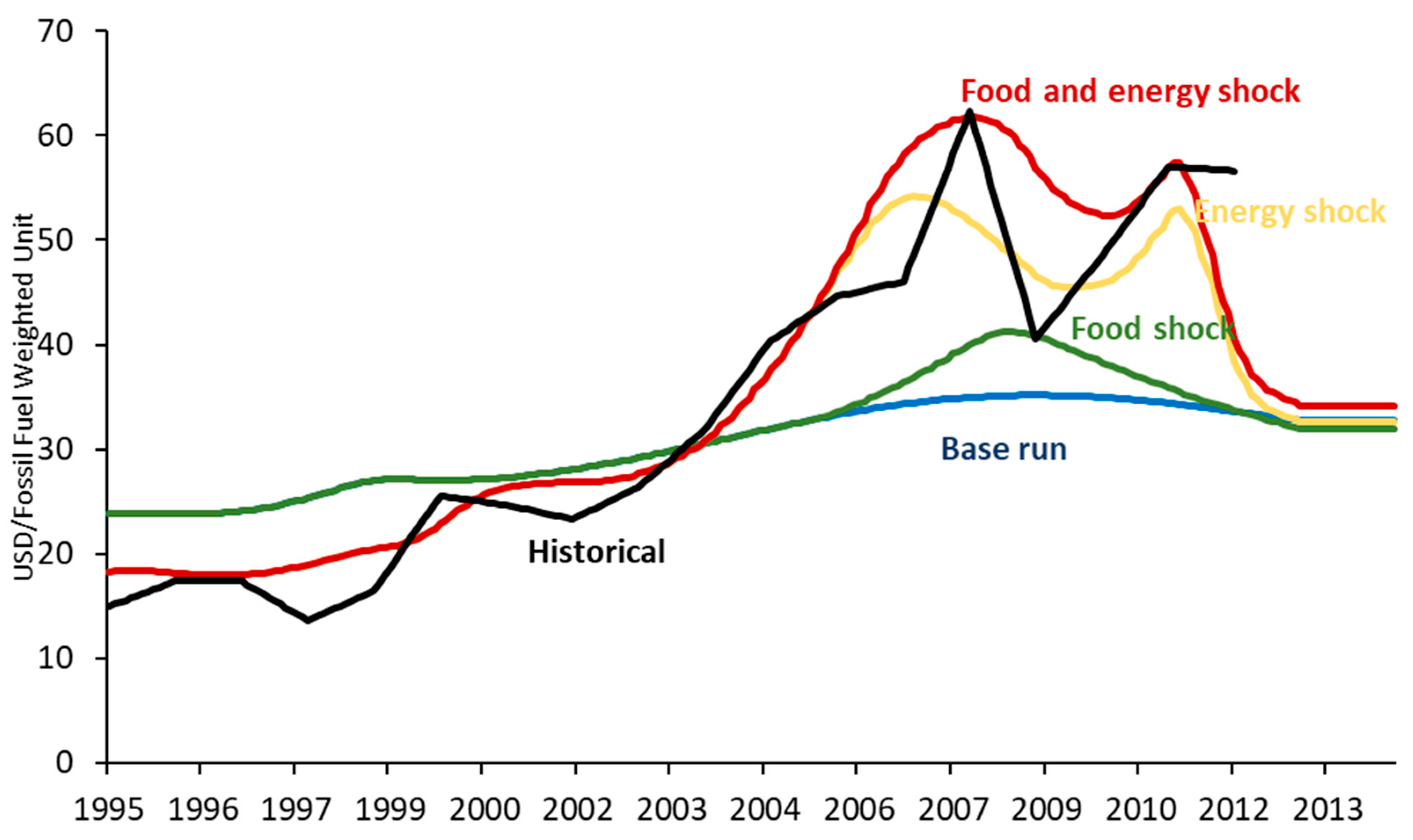
Figure 7.
Cereal commodity historic price data (own elaboration from [47]) compared to the base run scenario and shock scenarios of the model.
Figure 7.
Cereal commodity historic price data (own elaboration from [47]) compared to the base run scenario and shock scenarios of the model.


Table 1.
Summary of real and financial flows in the model.
| To | Households | Firms | Sovereign institutions | |||||
|---|---|---|---|---|---|---|---|---|
| From | Capital owners (H) | Workers (W) | Food (AC) | Energy (EN) | Goods and Capital (GC) | Government (GV) | Banks (B) | |
| Households | Capital owners (H) | - | - | Food demand and payments | Energy demand and payments | Goods and Capital demand and payments | Taxes on income | Borrowing, Debt retirement, payments for interest, and Savings deposits |
| Workers (W) | - | - | Food demand and payments | Energy demand and payments | Goods and Capital demand and payments | Taxes on income | Borrowing, Debt retirement and payments for interest | |
| Firms | Food (AC) | Dividends and food supply | Wages and food supply | - | Energy demand and payments | Capital demand and payments | Taxes on profit | Borrowing, Debt retirement and payments for interest |
| Energy (EN) | Dividends and energy supply | Wages and energy supply | Energy supply | Energy demand and payments | Energy supply | Taxes on profit | Borrowing, Debt retirement and payments for interest | |
| Goods and Capital (GC) | Dividends and goods and capital supply | Wages and Goods and Capital supply | Goods and Capital supply and Arable Land development | Goods and Capital supply | Goods and Capital supply | Taxes on profit | Borrowing, Debt retirement and payments for interest | |
| Sovereign institutions | Government (GV) | Government transfers as fraction of expenditure | Governments transfers as fraction of expenditure | Subsidies | Subsidies | - | - | Borrowing, Debt retirement and payments for interest |
| Banks (B) | Interest payments as a fraction of deposits on total money, Lending | Wages interest income remaining, Lending | Lending | Lending | Lending | Lending | Money supply | |
Table 2.
Balance sheet matrix of the closed system economy.
| Stock Variables | Sectors | Sum | ||||||
|---|---|---|---|---|---|---|---|---|
| Households | Firms | Sovereign Institutions | ||||||
| H | W | AC | EN | GC | GV | B | ||
| Value of capital assets | +CH | +CW | +AIAC + ALAC | +CEN | +CGC | +CH + CW + AIAC + ALAC + CEN + CGC | ||
| Liquidity | +MH | +MW | +MAC | +MEN | +MGC | +MGV | +MB | +MH + MW + MAC + MEN + MGC + MGV + MB |
| Debt | −DH= − (CH × FH) | −DW= − (CW × FW) | −DAC= − ((AIAC + ALAF) × FAC) | −DEN = − (CEN × FEN) | −DGC = − (CGC × FGC) | −DGV = BB | −DH-DW − DAC − DEN − DGC − DGV | |
| Deposits | +SH | −SB = − SH | 0 | |||||
| Equity | −EH = − (CH + MH + SH − DH) | −EW = − (CW + MW − DW) | −EAC = − (CAC + ALAC + MAC − DAC) | −EEN = − (CEN + MEN − DEN) | −EGC = − (CGC + MGC − DGC) | -EGV = − (MGV − DGV) | −EH − EW − EAC − EEN − EGC − EGV | |
| Bonds | +BB | +BB | ||||||
| Reserves | +RB | +RB | ||||||
| Loans | +LB = DH + DW + DAC + DEN + DGV | +LB | ||||||
| Debt money | −DMB | −DMB | ||||||
| Sum | 0 | 0 | 0 | 0 | 0 | 0 | 0 | 0 |
Legend sectors: “H”—Households Capital owners, “W”—Workers, “AC”—Agriculture, “EN”—Energy, “GC”—Good and Capital, “GV”—Government, “B”—Bank; Legend Variables: “Ci“—Capital Value stock in every sector, “AIAC“—Agricultural inputs in Agriculture sector (equivalent to Capital in other sectors), “ALAC“—Arable land in agriculture sector, “Mi“—Liquidity stock in every sector, “Di“—Debt Stock in every sector, “Fi“—Fraction of Debt to assets parameter in each sector, “BB“—Bonds owned by banks, “SH“—Savings for households, “SB“—Savings of households in Banks, “RB“—Reserves in Banks, “LB“—Loans from banks, “DMB“—Debt Money from banks.
© 2019 by the authors. Licensee MDPI, Basel, Switzerland. This article is an open access article distributed under the terms and conditions of the Creative Commons Attribution (CC BY) license (http://creativecommons.org/licenses/by/4.0/).
Share and Cite
MDPI and ACS Style
Pasqualino, R.; Monasterolo, I.; Jones, A. An Integrated Global Food and Energy Security System Dynamics Model for Addressing Systemic Risk. Sustainability 2019, 11, 3995. https://doi.org/10.3390/su11143995
AMA Style
Pasqualino R, Monasterolo I, Jones A. An Integrated Global Food and Energy Security System Dynamics Model for Addressing Systemic Risk. Sustainability. 2019; 11(14):3995. https://doi.org/10.3390/su11143995
Chicago/Turabian StylePasqualino, Roberto, Irene Monasterolo, and Aled Jones. 2019. "An Integrated Global Food and Energy Security System Dynamics Model for Addressing Systemic Risk" Sustainability 11, no. 14: 3995. https://doi.org/10.3390/su11143995
Note that from the first issue of 2016, this journal uses article numbers instead of page numbers. See further details here.