Mapping and Statistical Analysis of NO2 Concentration for Local Government Air Quality Regulation


Abstract
:1. Introduction
2. Method
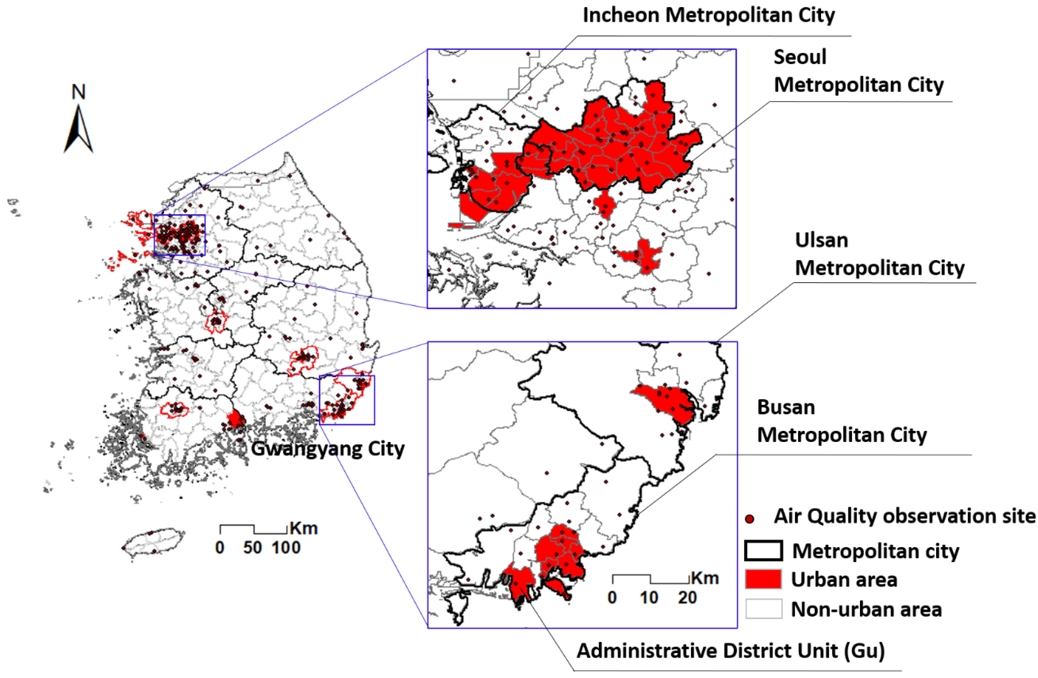
2.1. Study Area
2.2. Generation of NO2 Concentration Data
2.2.1. Monitoring NO2 Levels
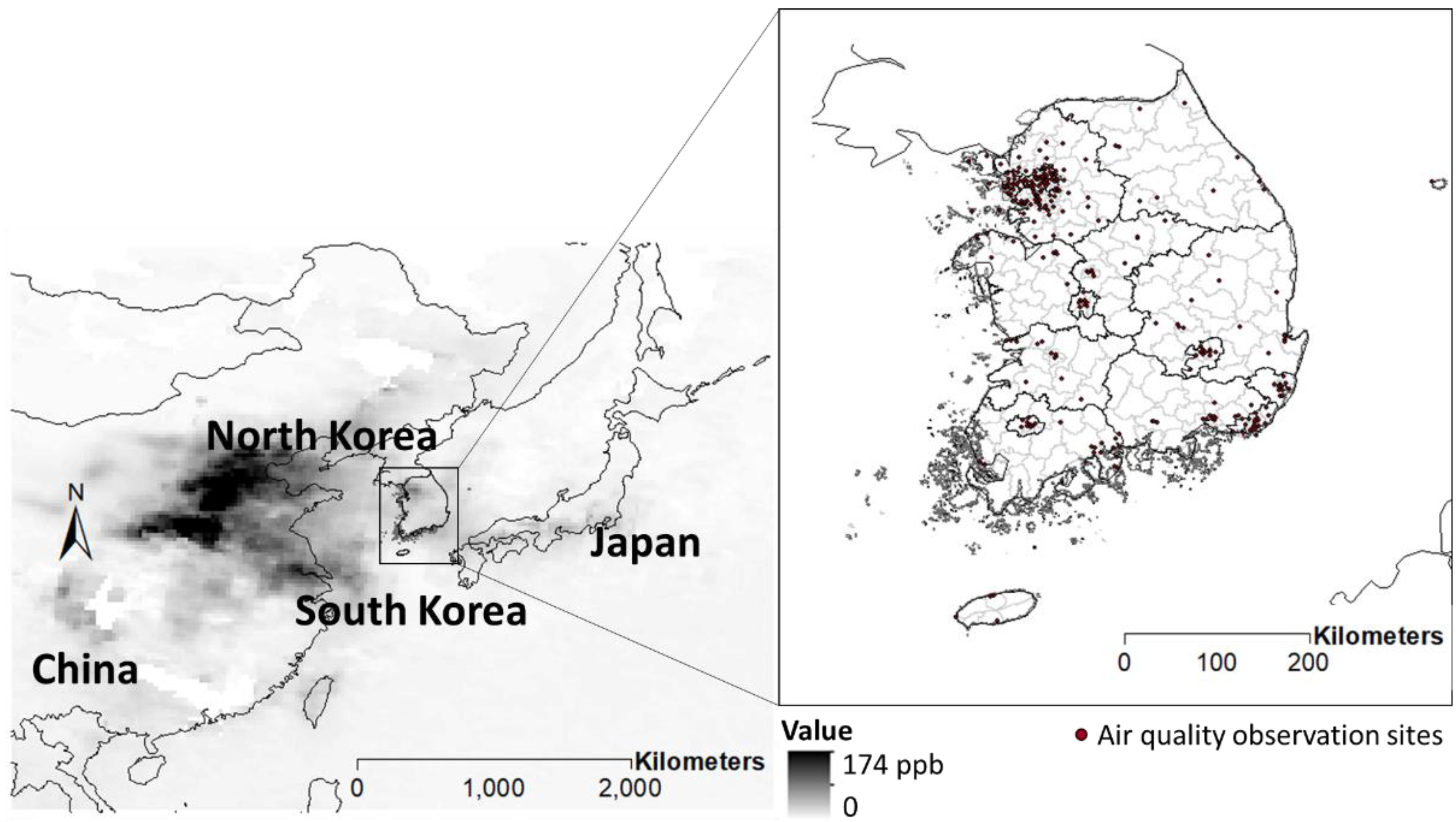
2.2.2. Satellite Images Used to Monitor NO2
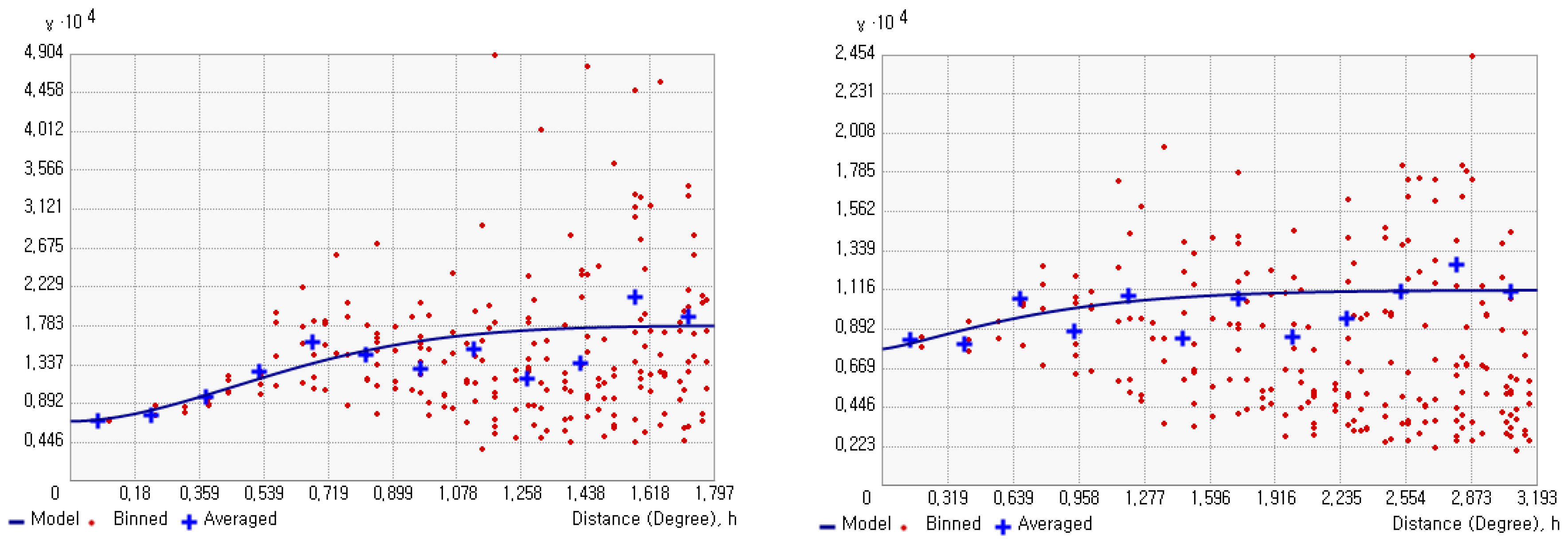
2.2.3. Geostatistical A Spatial Analysis: Cokriging
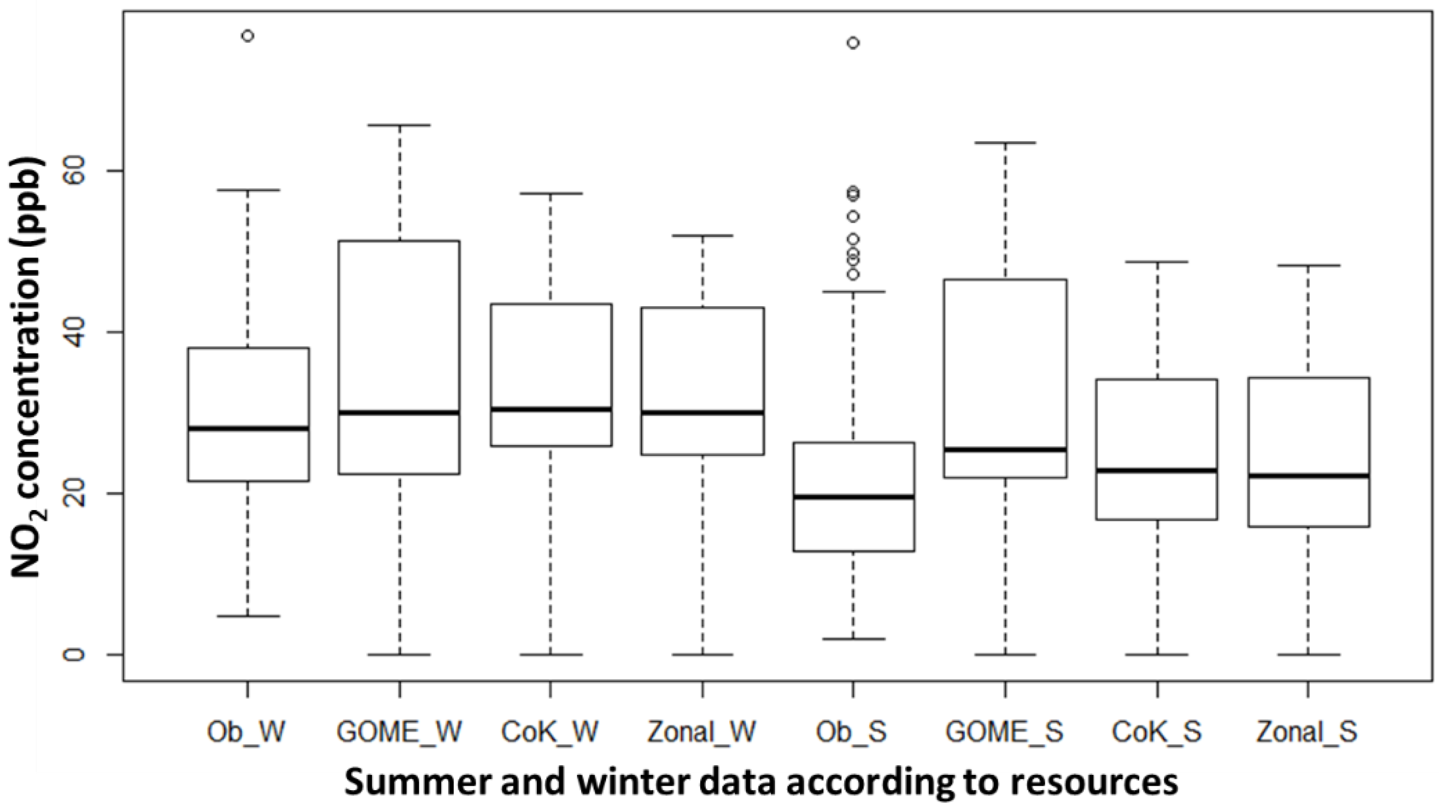
2.3. Comparison of Data Characteristics by Spatial Unit
2.4. Prediction of NO2 Concentrations by Administrative Unit Using A Land Use Regression Model
3. Results
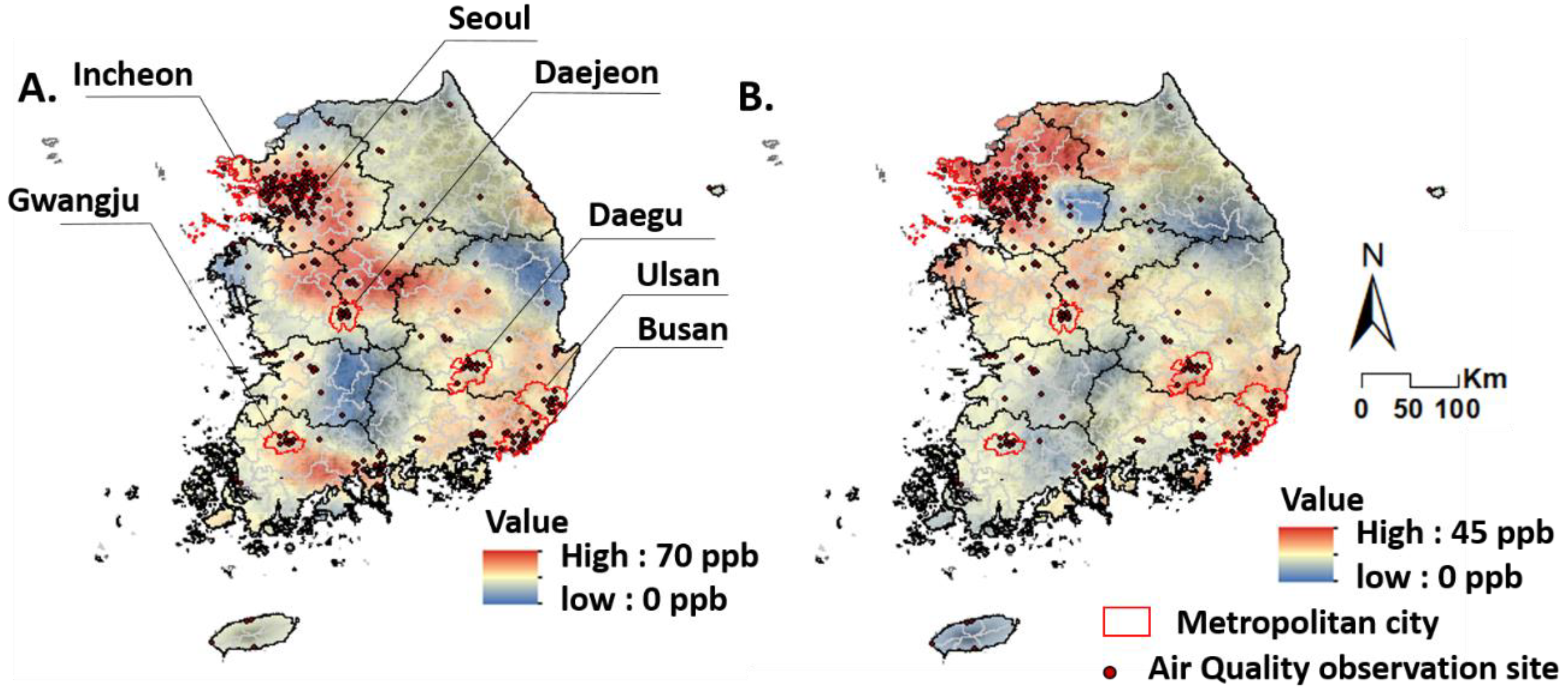
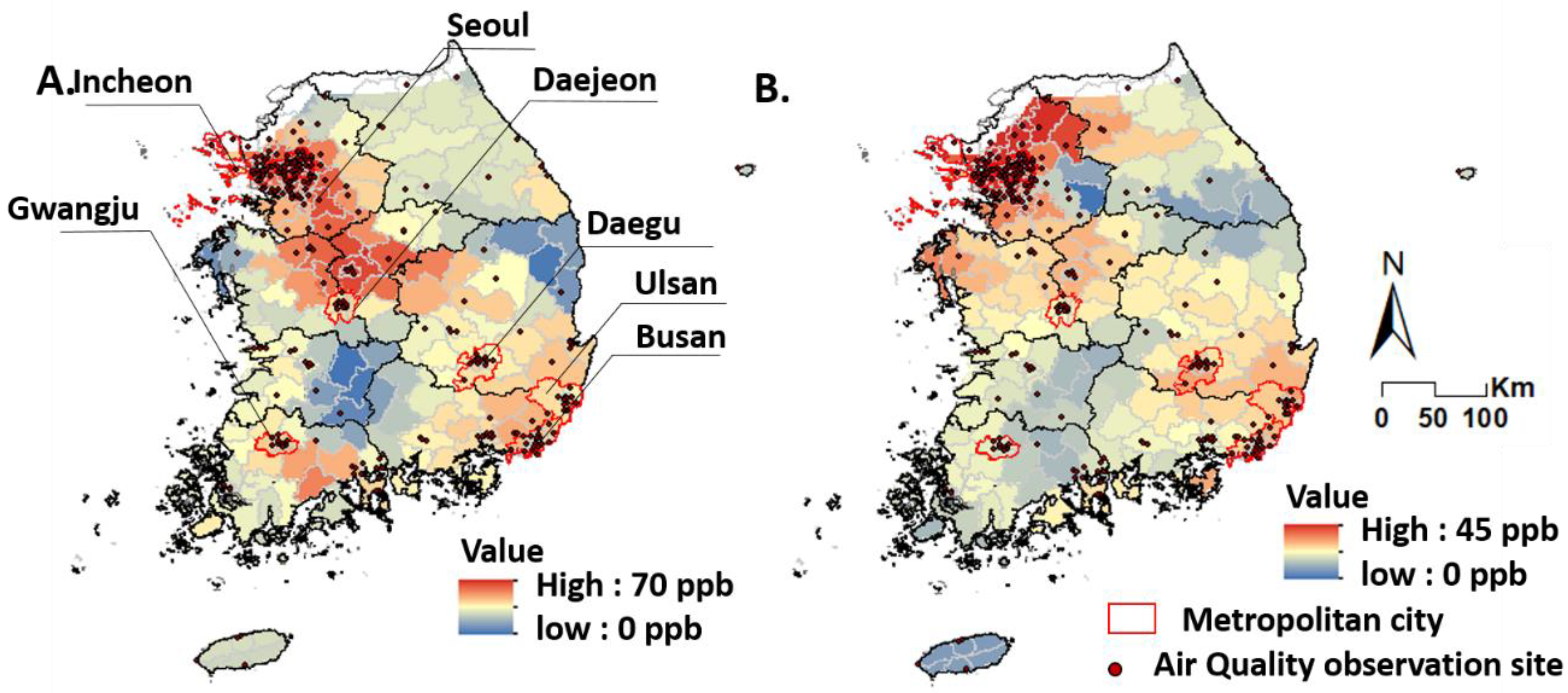
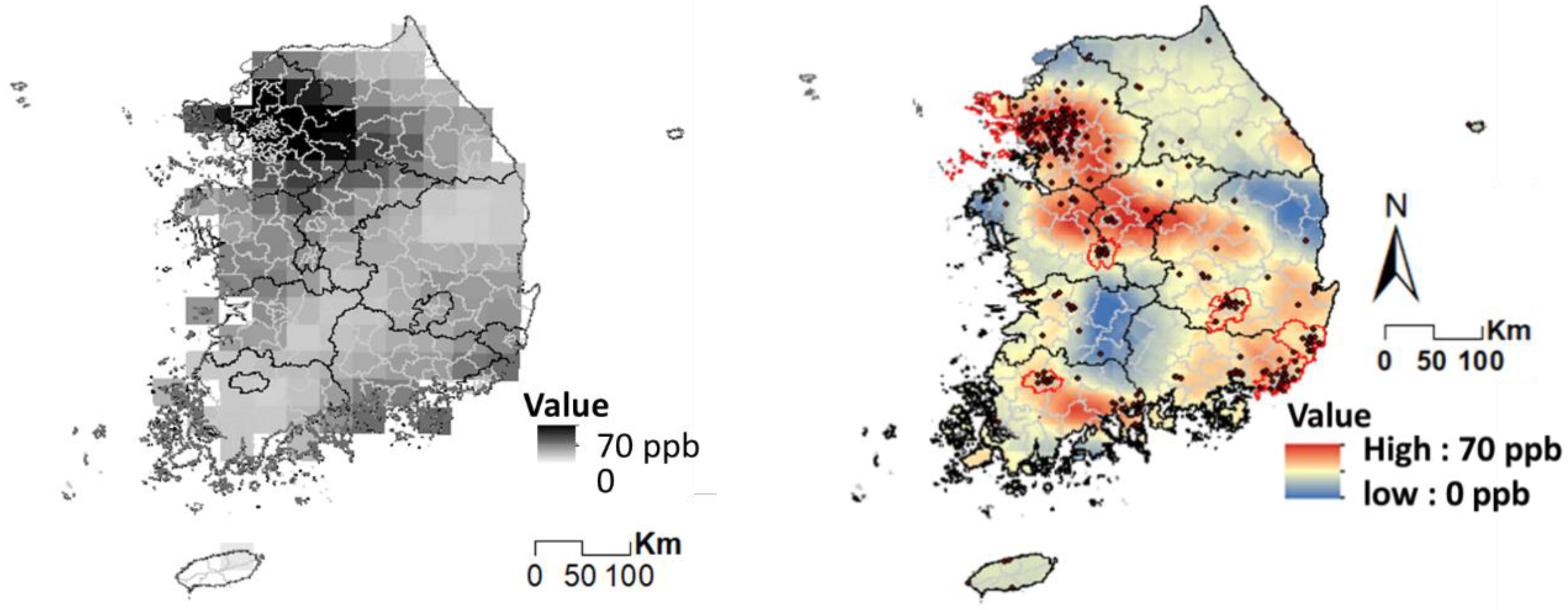
3.1. Nationwide NO2 Concentration
3.2. Analysis of the Accuracy of Nationwide NO2 Concentrations Measured by Administrative Unit
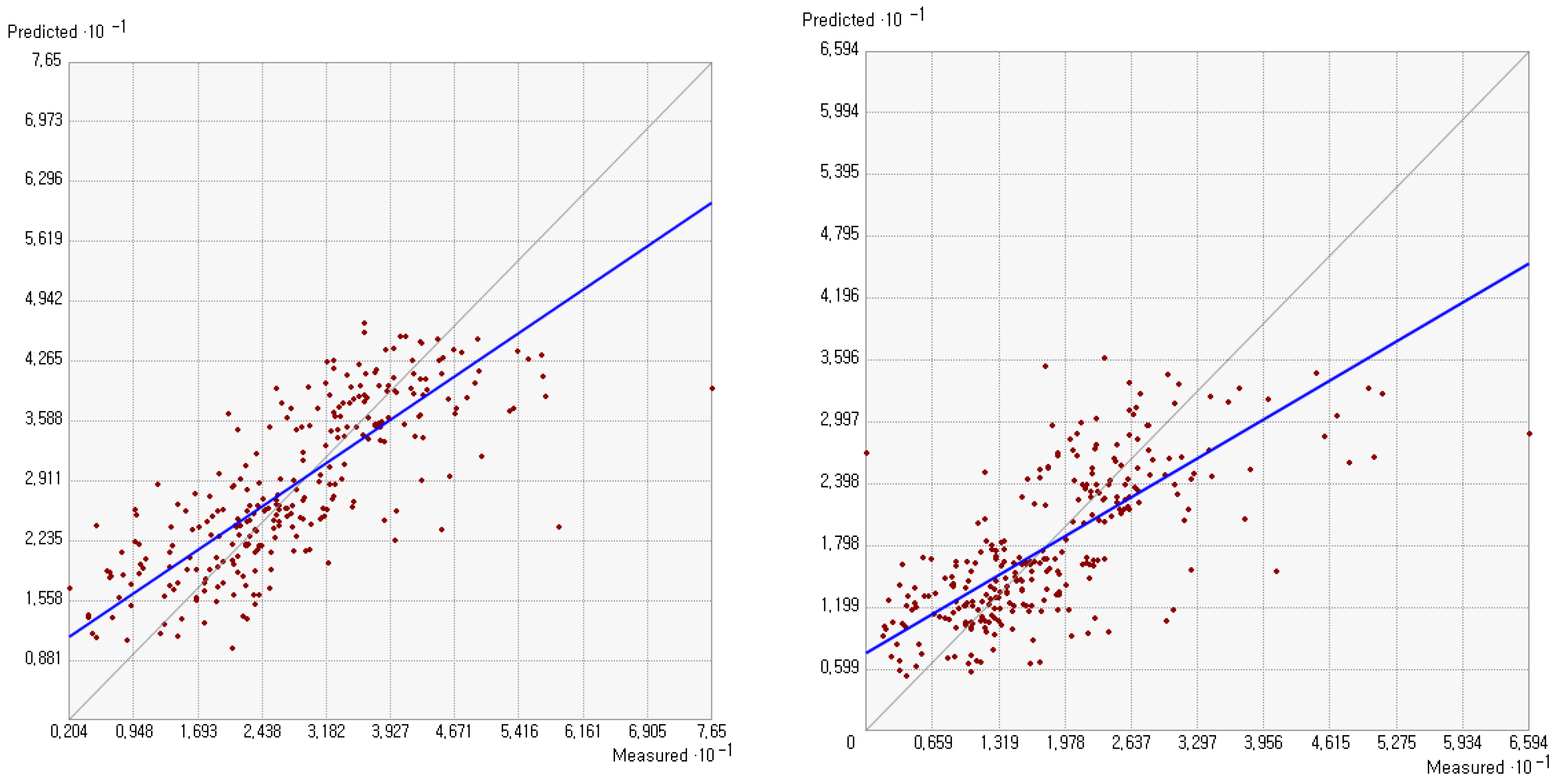
3.3. Analysis of NO2 Concentration Values Using LUR Models
4. Discussion
5. Conclusions
Author Contributions
Funding
Conflicts of Interest
Appendix A

Appendix B

References
- Lee, D.H.; An, S.S.; Song, H.M.; Park, O.H.; Park, K.S.; Seo, G.Y.; Cho, Y.G.; Kim, E.S. The effect of traffic volume on the air quality at monitoring sites in Gwangju. Korean Soc. Environ. Health 2014, 40, 204–214. [Google Scholar] [CrossRef]
- Borge, R.; Santiago, J.L.; Paz, D.; de la Martin, F.; Domingo, J.; Valdes, C.; Sanchez, B.; Rivas, E.; Rozas, M.T.; Lazaro, S.; et al. Application of a short term air quality action plan in Madrid(Spain) under a high-pollution episode-Part II: Assessment from multi-scale modelling. Sci. Total Environ. 2018, 635, 1574–1584. [Google Scholar] [CrossRef] [PubMed]
- Valks, P.; Pinardi, A.; Richter, A.; Lambert, J.-C.; Hao, N.; Loyola, D.; van Roozendael, M.; Emmadi, S. Operational total and tropospheric NO2 column retrieval for GOME-2. Atmos. Meas. Technol. 2011, 4, 1491–1514. [Google Scholar] [CrossRef]
- Streets, D.G.; Canty, T.; Carmichael, G.R.; de Foy, B.; Dickerson, R.R.; Duncan, B.N.; Edwards, D.P.; Haynes, J.A.; Henze, D.K.; Houyoux, M.R.; et al. Emissions estimation from satellite retrievals: A review of current capability. Atmos. Environ. 2013, 77, 1011–1042. [Google Scholar] [CrossRef] [Green Version]
- Duncan, B.N. , Lamsal, L.N.; Thompson, A.M.; Yoshida, Y.; Lu, Z.; Streets, D.G.; Hurwitz, M.M.; Pickering, K.E. A space-based, high-resolution view of notable changes in urban NOx pollution around the world (2005-2014). J. Geophysical Res. Atmos. 2015, 121, 976–996. [Google Scholar] [CrossRef]
- Cui, Y.; Zhang, W.; Bao, H.; Wang, C.; Cai, W.; Yu, J.; Streets, D.G. Spatiotemporal dynamics of nitrogen dioxide pollution and urban development: Satellite observations over China, 2005-2016, Resour. Conserv. Recycl. 2019, 142, 59–68. [Google Scholar] [CrossRef]
- European Environment Agency (EEA). Air quality in Europe-2018 report, EEA Technical report no 12/2018. ISSN 1977-8449. 2018. [Google Scholar]
- Kim, D.S.; Hwang, J.J. The origination mechanism of PM10 and methodology of identification for PM10 sources. Air Clean. Technol. 2002, 15, 38–53. [Google Scholar]
- Kim, Y.S.; Moon, J.S. A study on the relationship between air pollution and respiratory mortality. Atmos. Health Assoc. 1997, 23, 137–145. [Google Scholar]
- Seo, W.H.; Chang, S.S.; Kwon, H.J. Concentration of air pollutants and asthma in Taejon city. J. Environ. Health Sci. 2000, 26, 80–90. [Google Scholar]
- AEA Technology Environment. Damages per tonne emission of PM2.5, NH3, SO2, NOx and VOCs from each EU25 member State (excluding Cyprus) and surrounding seas. In Service Contract for Carrying out Cost-Benefit Analysis of Air Quality Related Issues, in particular in the Clean Air for Europe (CAFE) Programme; AEA Technology Environment: Oxon, UK, 2005; pp. 4–20. [Google Scholar]
- European Commission. Communication from the Commission to the European Parliament, the Council, the European Economic and Social Committee and the Committee of the Regions ‘A Europe that protects: Clean air for all’ (COM(2018) 330 final). Available online: http://ec.europa.eu/environment/air/pdf/clean_air_for_all.pdf (accessed on 9 July 2018).
- CAAC. Clean Air Alliance of China, State Council air pollution prevention and control action plan, issue II, October 2013 (English translation). Available online: http://en.cleanairchina.org/product/6346.html (accessed on 8 October 2015).
- Van Der A, R.J.; Mijling, B.; Ding, J.; Elissavet Koukouli, M.; Liu, F.; Li, Q.; Mao, H.; Theys, N. Cleaning up the air: effectiveness of air quality policy for SO2 and NOx emissions in China. Atmos. Chem. Phys. 2017, 17, 1775–1789. [Google Scholar] [CrossRef]
- Wang, S.; Xing, J.; Zhao, B.; Jang, C.; Hao, J. Effectiveness of national air pollution control policies on the air quality in metropolitan areas of China. J. Environ. Sci. 2014, 26, 13–22. [Google Scholar] [CrossRef]
- Park, R.S.; Han, K.M.; Song, C.H.; Park, M.E.; Lee, S.J.; Hong, S.Y.; Kim, J.; Woo, J.H. Current status and development of modeling techniques for forecasting and monitoring of air quality over east Asia. J. Korean Soc. Atmos. Environ. 2013, 29, 407–438. [Google Scholar] [CrossRef]
- Kokhanovsky, A.A.; von Hoyningen-Huene, W.; Burrow, J.P. Atmospheric aerosol load from space. Atmos. Res. 2006, 81, 176–185. [Google Scholar] [CrossRef]
- Sahsuvaroglu, T.; Su, J.G.; Brook, J.; Burnett, M.L.; Jerrett, M. Predicting personal nitrogen dioxide exposure in an elderly population: Integrating residential indoor and outdoor measurements, Fixed-site ambient pollution concentrations, modeled pollutant levels, and time-activity patterns. J. Toxicol. Environ. Health Part A 2009, 72, 1520–1533. [Google Scholar] [CrossRef] [PubMed]
- Meng, X.; Chen, L.; Cai, J.; Zou, B.; Wu, C.-F.; Fu, Q.; Zhang, Y.; Liu, Y.; Kan, H. A land use regression model for estimating the NO2 concentration in Shanghai, China. Environ. Res. 2015, 137, 308–315. [Google Scholar] [CrossRef] [PubMed]
- Hatzopoulou, M.; Valois, M.F.; Mihele, C.; Lu, G.; Bagg, S.; Minet, L.; Brook, J. Robustness of land-use regression models developed from mobile air pollutant measurements. Environ. Sci. Technol. 2017, 51, 3938–3947. [Google Scholar] [CrossRef]
- Rho, Y. Pattern analysis and mapping of urban air pollution using exposure time metric and mortality caused by cardiovascular and respiratory illnesses. J. Environ. Policy Adm. 2017, 25, 21–48. [Google Scholar]
- Choi, G.; Bell, M.L.; Lee, J.T. A study on modeling nitrogen dioxide concentrations using land-use regression and conventionally used exposure assessment methods. Environ. Res. Lett. 2017, 12, 1–11. [Google Scholar] [CrossRef]
- Beelen, R.; Hoek, G.; Vienneau, D.; Eeftens, M.; Dimakopoulou, K.; Pedeli, X.; Tsai, M.-Y.; Künzli, N.; Schikowski, T.; Marcon, A.; et al. Development of NO2 and NOx land use regression models for estimating air pollution exposure in 36 study areas in Europe—The ESCAPE project. Atmos. Environ. 2013, 72, 10–23. [Google Scholar] [CrossRef]
- Hoek, G.; Beelen, R.; de Hoogh, K.; Vienneau, D.; Gulliver, J.; Fischer, P.; Briggs, D. A review of land-use regression models to assess spatial variation of outdoor air pollution. Atmos. Environ. 2008, 42, 7561–7578. [Google Scholar] [CrossRef]
- Famoso, F.; Wilson, J.; Monforte, P.; Lanzafame, R.; Brusca, S.; Lulla, V. Measurement and modeling of ground-level ozone concentration in Catania, Italy using biophysical remote sensing and GIS. Int. J. Appl. Eng. Res. 2017, 12, 10551–10562. [Google Scholar]
- Cowie, C.T.; Garden, F.; Jegasothy, E.; Knibbs, L.D.; Hanigan, I.; Morley, D.; Hansell, A.; Hoek, G.; Marks, G.B. Comparison of model estimates from an intra-city land use regression model with a national satellite-LUR and a regional Bayesian Maximum Entropy model, in estimating NO2 for a birth cohort in Sydney, Australia. Environ. Res. 2019, 174, 24–34. [Google Scholar] [CrossRef] [PubMed]
- Kim, S.K.; Han, J.S.; Yeo, S.Y.; Sul, S.H.; Lee, H.G.; Lee, G.M. Standard Work Procedures for Building Basic Data on National Air Pollutant Emissions: Estimated Emissions by 2013. Natl. Inst. Environ. Res. 2016, NIER-GP2016-062, 178–179. [Google Scholar]
- Irie, H.; Boersma, K.F.; Kanaya, Y.; Takashima, H.; Pan, X.; Wang, Z.F. Quantitative bias estimates for tropospheric NO2 columns retrieved from SCIAMACHY, OMI, and GOME-2 using a common standard for East Asia. Atmos. Meas. Technol. 2012, 5, 2403–2411. [Google Scholar] [CrossRef]
- Constantin, D.E.; Voiculescu, M.; Georgescu, L. Satellite Observations of NO2 Trend over Romania. Sci. World J. 2013, 2013, 1–10. [Google Scholar] [CrossRef] [PubMed]
- Goovaerts, P. Geostatistics for Natural Resources Evaluation; Oxford University Press: Oxford, UK, 1997; pp. 185–258. [Google Scholar]
- Choi, J.H.; Kim, B.J. A study for applicability of cokriging techniques for estimating the real transaction price of land. Korean Soc. Geospat. Inform. Syst. 2015, 23, 55–63. [Google Scholar]
- Lim, C.-H.; Ryu, D.-H.; Song, C.-H.; Zhu, Y.-Y.; Lee, W.-K.; Kim, M.-S. Semi-variogram precise spatio-temporal distribution of weather condition using semi-variogram in small scale recreation forest. J. Korean Assoc. Geogr. Inf. Stud. 2015, 18, 63–75. [Google Scholar] [CrossRef]
- Ghorbani, A.; Moghaddam, S.M.; Majd, K.H.; Dadgar, N. Spatial variation analysis of soil properties using spatial statistics: a case study in the region of Sabalan mountain, Iran. J. Prot. Mt. Areas Res. Manag. 2018, 10, 70–80. [Google Scholar] [CrossRef] [Green Version]
- Ma, X.; Journel, A.G. An expanded GSLIB cokriging program allowing for tow Markov models. Comput. Geosci. 1999, 25, 627–639. [Google Scholar] [CrossRef]
- He, H.-D. Multifractal analysis of interactive patterns between meteorological factors and pollutants in urban and rural areas. Atmos. Environ. 2017, 149, 47–54. [Google Scholar] [CrossRef]
- Cordioli, M.; Pironi, C.; de Munari, E.; Marmiroli, N.; Lauriola, P.; Ranzi, A. Combining land use regression models and fixed site monitoring to reconstruct spatiotemporal variability of NO2 concentrations over a wide geographical area, Sci. Total Environ. 2017, 574, 1075–1084. [Google Scholar] [CrossRef] [PubMed]
- Oh, K.; Koo, J.; Cho, C. The effects of urban spatial elements on local air pollution. J. Korea Plan. Assoc. 2005, 40, 159–170. [Google Scholar]
- Kim, J.C. Temporal and spatial variation and characteristics of ambient air quality in urban areas in Gyeonggi Province. Korean J. Environ. Health Sci. 2012, 38, 269–276. [Google Scholar] [CrossRef]
- Antanasijevic, D.; Pocajt, V.; Peric-Grujic, A.; Ristic, M. Multiple-input-multiple-output general regression neural networks model for the simultaneous estimation of traffic-related air pollutant emissions. Atmos. Pollut. Res. 2018, 9, 388–397. [Google Scholar] [CrossRef]
- Honlnicki, P.; Kaluszko, A.; Nahorski, Z.; Stankiewicz, K.; Trapp, W. Air quality modeling for Warsaw agglomeration. Arch. Environ. Prot. 2017, 43, 48–64. [Google Scholar] [CrossRef] [Green Version]
- Ministry of Environment. National Sustainability Report, Sustainable Development Basic Plan Check and Indicator Evaluation Results. Sustain. Dev. Comm. 2016, 11-14800000-001344-01, 68–69. [Google Scholar]
- Baek, S.G.; Jang, D.H. Evaluation for applicability of cokriging for high resolution spatial mapping of temperature and rainfall. Clim. Stud. 2011, 6, 242–253. [Google Scholar]
- Wolf, K.; Cyrys, J.; Harcinikova, T.; Gu, J.; Kusch, T.; Hampel, R.; Schneider, A.; Peters, A. Land use regression modeling of ultrafine particles, ozone, nitrogen oxides and markers of particulate matter pollution in Augsburg, Germany. Sci. Total Environ. 2017, 579, 1531–1540. [Google Scholar] [CrossRef] [Green Version]
- Anquetin, S.; Guilbaud, C.; Chollet, J.P. Thermal valley inversion impact on the dispersion of a passive pollutant in a complex mountainous area. Atmos. Environ. 1999, 33, 3953–3959. [Google Scholar] [CrossRef]
- Joo, H.S.; Kim, S.C.; Bae, S.Y. Impacts of green spaces on air quality. Korea Environ. Inst. 2005, RE-15, 55–72. [Google Scholar]
- Goldberg, D.L.; Lamsal, L.N.; Loughner, C.P.; Swartz, W.H.; Lu, Z.; Streets, D.G. A high-resolution and observationally constrained OMI NO2 satellite retrieval. Atmos. Chem. Phys. 2017, 17, 11403–11421. [Google Scholar] [CrossRef]
- Wang, Y.; Beirle, S.; Lampel, J.; Koukouli, M.; de Smedt, I.; Theys, N.; Li, A.; Wu, D.; Xie, P.; Liu, C.; et al. Validation of OMI, GOME-2A and GOME-2B tropospheric NO2, SO2 and HCHO products using MAX-DOAS observations from 2011 to 2014 in Wuxi, China: Investigation of the effects of priori profiles and aerosols on the satellite products. Atmos. Chem. Phys. 2017, 17, 5007–5033. [Google Scholar] [CrossRef]
- Bechle, M.J.; Millet, D.B.; Marshall, J.D. National spatiotemporal exposure surface for NO2: Monthly scaling of a satellite-derived land-use regression, 2000-2010, Environ. Sci. Technol. 2015, 49, 12297–12305. [Google Scholar] [CrossRef] [PubMed]
- Anand, J.S.; Monks, P.S. Estimating daily surface NO2 concentrations from satellite data: a case study over Hong Kong using land use regression models, Atmos. Chem. Phys. 2017, 17, 8211–8230. [Google Scholar]
- Rahman, M.M.; Yeganeh, B.; Clifford, S.; Knibbs, L.D.; Morawska, L. Development of a land use regression model for daily NO2 and NOx concentrations in the Brisbane metropolitan area, Australia, Environ. Model. Softw. 2017, 95, 168–179. [Google Scholar] [CrossRef]
- Park, J.-C.; Kim, M.-K. Comparison of precipitation distributions in precipitation data sets representing 1km spatial resolution over south Korea produced by PRISM, IDW, and cokriging. J. Korean Assoc. Geogr. Inf. Stud. 2013, 16, 147–163. [Google Scholar] [CrossRef]
- Rahman, A.; Luo, C.; Khan, M.H.R.; Ke, J.; Thilakanayaka, V.; Kumar, S. Influence of atmospheric PM2.5, PM10, O3, CO, NO2, SO2, and meteorological factors on the concentration of airborne pollen in Guangzhou, China. Atmos. Environ. 2019, 212, 290–304. [Google Scholar] [CrossRef]
- Xie, M.; Piedrahita, R.; Dutton, S.J.; Milford, J.B.; Hemann, J.G.; Peel, J.L.; Miller, S.L.; Kim, S.Y.; Vedal, S.; Sheppards, L.; et al. Positive matrix factorization of a 32-month series of daily PM2.5 speciation data with incorporation of temperature stratification. Atmos. Environ. 2013, 65, 11–20. [Google Scholar] [CrossRef] [Green Version]
- Davies, H.W.; Vlaanderen, J.; Henderson, S.; Brauer, M. Correlation between co-exposures to noise and air pollution from traffic sources. Occup. Environ. Med. 2009, 66, 347–350. [Google Scholar] [CrossRef]
- Itahashi, S.; Uno, I.; Irie, H.; Kurokawa, J.-I.; Ohara, T. Regional modeling of tropospheric NO2 vertical column density over East Asia during the period 2000–2010: comparison with multisatellite observations. Atmos. Chem. Phys. 2014, 14, 3623–3635. [Google Scholar] [CrossRef]
- Mijling, B.; van der A, R.J.; Zhang, Q. Regional nitrogen oxides emission trends in East Asia observed from space. Atmos. Chem. Phys. 2013, 13, 12003–12012. [Google Scholar] [CrossRef] [Green Version]


| Predictor Variable | Name | Effect | Other Comments | |
|---|---|---|---|---|
| Seasonal factors | ||||
| Season | Season | Summer = 1, winter = 0 | ||
| Emission factors | ||||
| Percentage of residential area | R_Res | + | Residential area by administrative district/Area of each administrative district *100 | |
| Percentage of industrial complex area | R_Ind | + | Industrial complex area by administrative district/Area of each administrative district *100 | |
| Percentage of commercial area | R_Com | + | Commercial area by administrative district/Area of each administrative district *100 | |
| Percentage of cultural recreation area | R_Cul | + | Area of cultural recreation area by administrative district/Area of each administrative district *100 | |
| Percentage of public facilities area | R_Pub | + | Area of public facilities by administrative district /Area of each administrative district *100 | |
| Percentage of urbanization area | R_Urban | + | Area of urbanization by administrative district /Area of each administrative district *100 | |
| Length of roads | Road_Length | + | Length of roads (km)/Area of each administrative district (km2) | |
| Percentage of population | R_Pop | + | Population/Area of each administrative district *100 | |
| Road length per unit population | RL/Pop | + | Road_Length/R_Pop | |
| Reduction factors | ||||
| Percentage of paddy field | R_Paddy | - | Area of paddy fields within an administrative district /Area of each administrative district *100 | |
| Percentage of field | R_Field | - | Area of fields within administrative district /Area of each administrative district *100 | |
| NDVI | NDVI | - | Using zonal statistics of ArcGIS, we derive the monthly average NDVI data of the Moderate Resolution Imaging Spectroradiometer (MODIS) in the cell using the average for the administrative district | |
| Coniferous forest ratio | R_Coni | - | Coniferous forest area by administrative district / Area of administrative district *100 | |
| Deciduous forest ratio | R_Deci | -/+ | Deciduous forest area by administrative district /Area of administrative district *100 | |
| Mixed forest ratio | R_Mixed | -/+ | Mixed forest area by administrative district /Area of administrative district *100 | |
| Forest ratio | R_Forest | - | Forest area by administrative district /Area of administrative district *100 | |
| Topographical factors | ||||
| DEM | DEM_std | - | Using the zonal statistics of ArcGIS, we derive the standard deviation value of the DEM for each cell as the average value by administrative unit | |
| Urban Regions | (Adj. R2 = 0.335) | ||||||
| Model | Unstandardized Coefficients | Standardized Coefficients | t | Sig. | Collinearity Statistics | ||
| B | Std. Error | Beta | Tolerance | VIF | |||
| (Constant) | 41.360 | 3.700 | 11.179 | 0.000 | |||
| NDVI | −29.385 | 5.409 | −0.460 | −5.433 | 0.000 | 0.918 | 1.089 |
| RL_Pop | 3.565 | 1.155 | 0.261 | 3.087 | 0.003 | 0.918 | 1.089 |
| Non-Urban Regions | (Adj. R2 = 0.526) | ||||||
| Model | Unstandardized Coefficients | Standardized Coefficients | t | Sig. | Collinearity Statistics | ||
| B | Std. Error | Beta | Tolerance | VIF | |||
| (Constant) | 28.403 | 1.184 | 23.998 | 0.000 | |||
| NDVI | −22.593 | 1.689 | −0.471 | −13.378 | 0.000 | 0.954 | 1.048 |
| RL_Pop | 9.185 | 0.699 | 0.462 | 13.131 | 0.000 | 0.954 | 1.048 |
© 2019 by the authors. Licensee MDPI, Basel, Switzerland. This article is an open access article distributed under the terms and conditions of the Creative Commons Attribution (CC BY) license (http://creativecommons.org/licenses/by/4.0/).
Share and Cite
Ryu, J.; Park, C.; Jeon, S.W. Mapping and Statistical Analysis of NO2 Concentration for Local Government Air Quality Regulation. Sustainability 2019, 11, 3809. https://doi.org/10.3390/su11143809
Ryu J, Park C, Jeon SW. Mapping and Statistical Analysis of NO2 Concentration for Local Government Air Quality Regulation. Sustainability. 2019; 11(14):3809. https://doi.org/10.3390/su11143809
Chicago/Turabian StyleRyu, Jieun, Chan Park, and Seong Woo Jeon. 2019. "Mapping and Statistical Analysis of NO2 Concentration for Local Government Air Quality Regulation" Sustainability 11, no. 14: 3809. https://doi.org/10.3390/su11143809
APA StyleRyu, J., Park, C., & Jeon, S. W. (2019). Mapping and Statistical Analysis of NO2 Concentration for Local Government Air Quality Regulation. Sustainability, 11(14), 3809. https://doi.org/10.3390/su11143809