Article

Monitoring Spatial Changes in Manufacturing Firms in Seoul Metropolitan Area Using Firm Life Cycle and Locational Factors

1
The Department of Urban Planning and Design, The University of Seoul, Seoul 02504, Korea
2
The Department of Land Economy, The University of Cambridge, 19 Silver Street, Cambridge CB3 9EP, UK
*
Author to whom correspondence should be addressed.
Sustainability 2019, 11(14), 3808; https://doi.org/10.3390/su11143808
Submission received: 3 May 2019 / Revised: 1 July 2019 / Accepted: 3 July 2019 / Published: 11 July 2019

Abstract

:
This paper diagnoses the development of the manufacturing industry in the Seoul Metropolitan Area (SMA) using portfolio and regression analyses. Following the life-cycle perspective, four types of spatial changes of firms have been identified, namely firm formation, inflow, outflow, and dissolution, which are applied to analyze the manufacturing development in SMA. For portfolio analysis, we propose the Net Formation Index and Net Inflow Index to measure the spatial changes of firms at the city level. The two indices facilitate horizontal comparison among cities in SMA in terms of firm growth from new opening and relocation. Using spatial regression analysis, we identify significant location factors that contribute to firm change patterns. Our tests show that a high level of industrial specialization (measured by location quotient) has a dual effect. On the one hand, high level specialization attracts new or inflow firms, particularly in the light and high-tech manufacturing industries. On the other hand, it leads to an increased number of closed or outflow firms, plausibly due to increased competition among local firms. The proposed methods can be applied to diagnose industrial development in clusters of inter-connected cities and design policy tools to boost the local industry.

1. Introduction

Firms play an important role in cities [1,2]. They provide not only jobs for the population but also various goods and services to the city. Therefore, understanding the change of firms is important for the employment growth and the quality of life in cities. Combining the spatial and the life-cycle perspective, this paper investigates the changes in manufacturing firms in the Seoul Metropolitan Area (SMA) using portfolio analysis and spatial regression. The spatial perspective concerns the location and relocation of firms and the life-cycle perspective involves the establishment, growth/decline and possible closure of firms. The necessity of combining the spatial and the life-cycle perspective is that a firm relocated into (out from) a city may be easily miscounted as a new (closed) firm in aggregate firm data. This error is particularly relevant if the study area is at city-region level where firms may relocate across a cluster of interconnected cities. Our data for SMA shows that more than 10% of manufacturing firms in SMA have conducted inter-city relocation within the one-year period 2009–2010 [3,4].
The primary objective of the paper is to provide a systematic diagnosis of the development of manufacturing firms across SMA. The proposed research design consists of two analytical sections, i.e., the diagrammatic portfolio analysis and the spatial regression. The portfolio analysis provides a readily understandable diagram which plots cities based on two firm development indices derived from empirical data, i.e., the Net Formation Index and Net Firm Inflow Index. The diagram enables a visualized overview of cities within a city region in terms of the demographic changes of firms. The subsequent spatial regression aims to investigate the locational factors that may lead to the observed change patterns revealed in the portfolio analysis. The potential issue of spatial autocorrelation is discussed in detail through comprehensive model selection tests based on empirical data. The research method represents a new approach for investigating the spatial and demographic changes of firms across a wide city region.
The structure of the paper is as follows. In the next section, we present a brief review of the literature on spatial changes of firms, which leads to the discussion of the research design and data in Section 3. Section 4 presents the portfolio analysis by industry type, and Section 5 discusses the regression analysis. Concluding remarks are presented in Section 6.

2. Literature Review

Extensive research has been conducted to understand the mechanisms of firm location choices. In particular, the location choices of new firms have been a central research topic [5,6,7], reflecting the need to understand and promote industry development through targeted policy instruments. Many studies in this field have been focused on modeling the spatial changes of firms. For instance, Arauzo-Carod et al. [5] review this research strand and identify two main methodology types. First, the firm-based approach emphasizes the behavioral foundations for a firm’s location decision and models the decision with firm-specific data together with other locational factors. Micro-simulation methods, such as agent-based modeling, have been used to simulate firm behavior [8,9]. Second, count models are used to analyze the spatial pattern of firms across a study area. As pointed out by Arauzo-Carod et al. [5], while the firm-based approach has a sound behavioral basis, the limitations on firm-level data will largely undermine its advantages in practical applications. The second approach (i.e., count models), explicitly embraces the spatial dimension and identifies the locational factors that affect a firm’s decisions [10,11]. In other words, the count model approach explains why some locations are more attractive than others. Sophisticated statistical models have been put forward to identify the key factors for firm location choices [2,12,13,14,15].
Studies on firm location choices tend to use the total number of firms (or new firms) as the main indicator to analyze the status of an industry in a city [8,12,16,17,18,19,20]. However, this approach has several limitations. For example, if the total number of firms in a city remains unchanged, it may refer to distinct development situations—a stable industry or a churning industry with a large number of new and closed firms. In addition, the increase of firms in one city may be accompanied by a decreased number of firms in another city due to inter-city firm relocation—such information, though important, is often missed in aggregate firm count data.
Another important line of research investigates the change of firms from the life-cycle perspective, i.e., the demography of firms [21,22,23,24,25]. Along the life-cycle development of firms, some changes may feature an explicit spatial dimension. For example, the creation of a firm involves an initial choice of business location. During the growth or decline stages of firm development, firms may consider relocating for various reasons. Economic incentives may prompt firms to move closer to the consumer and/or labor market to reduce production costs. Other inside-the-firm factors may also lead to relocation. However, such factors are relatively difficult to trace using conventional data sources. Empirical data from the Netherlands suggest that firm relocation is not rare and has been more frequent since the 1990s [26]. Multiple relocations over the firm life cycle are also observed in the Dutch dataset. This finding suggests that it is important to examine the breakdown of firm changes in order to understand the full picture of the industry development in a city.
In addition, a firm’s location decision is an active action for profit maximization. Various factors influence this decision. Thus, the factors of choice that determine a firm’s location have been numerous for a long time [25,27]. One of the most frequently used variables, which is considered an important variable in advanced studies, is related to transportation facilities, such as main roads, railroads, subways, airports, and harbors [9,15,25,28,29,30,31,32,33]. The reason for this is based on the concept of minimal transportation cost in Weber’s “Theory of the Location of Industries” [34]. Furthermore, transport costs play a very important role in determining the unit product cost based on the cost of the supply of raw materials and the movement of products. The next very important factor studied in market-related factors [15,29,31,35,36,37,38,39] includes land price and rent based on von Thünen’s theory of location in his book The Isolated State. This is also essential in determining the unit price of a product. In addition, in location factors, the market scale was handled as population or employees. The following factors are related to labor [2,15,28,30,35]. This factor covered the easy availability of quality labor and the level of education, such as the educational background of the workforce. Tax and finance-related government support variables were also studied for the location decision of the firms [2,25,35]. However, this variable has many limitations in collecting and quantifying data. In a relatively recent study, agglomeration-related variables were studied as an important factor for industrial firms [40]. The most representative index for agglomeration effect is the Location Quotient (LQ) index, which indicates how an industry is relatively concentrated in the city. Finally, there are variables for industrial buildings available in the city [40,41]. Although this variable is very important as an actual physical variable for a firm to move in, it has not been used in many studies because of the difficulty in obtaining data.
This paper builds on the count model approach and incorporates the following extensions. First, while most of the count model papers are focused on new firms or total number of firms, this paper investigates firm changes from the life-cycle perspective, e.g., the formation, closure, and possible relocations of firms. Second, for firm relocation, the observed over 10% inter-city relocation rate of manufacturing firms in SMA suggests that the city region, rather a single city, is the appropriate spatial scale for studying spatial change of firms in a metropolitan area. This paper thus expands the study area to a wide city region, which includes a cluster of inter-connected cities. Third, the paper combines the diagrammatic portfolio analysis with the spatial regression—the portfolio analysis provides a consistent and visually understandable comparison of cities in terms of the development of local manufacturing firms.

3. Research Design and Data

3.1. Research Design

This paper aims to diagnose the development of manufacturing firms across localities in the Seoul Metropolitan Area from a life-cycle perspective. We first conceptualize the four types of spatial changes of firms along its life-cycle development. Two analytical indices are then proposed based on the four types of spatial changes, which decompose the aggregate firm count changes into two distinct components, i.e., local formation/closure and inter-city migration. Portfolio analysis is then conducted to visually categorize localities in the SMA in terms of the manufacturing development by sector segment. To explore how locational factors may affect the observed patterns of firm changes, the research follows established method for empirically selecting the appropriate regression model for each type of spatial change and each sector segment. The combination of the life-cycle perspective, extended portfolio analysis, and spatial regression models represents a new analytical strategy for understanding the varying industrial development patterns across a wide city region.

3.1.1. Life-Cycle Perspective

The literature tends to classify the firm life-cycle into four categories: Formation, growth, decline, and dissolution [11,12,13,14]. The possible relationships between the life-cycle and spatial changes during the growth and decline phases of firms are typically in the form of relocations or migrations [17], i.e., inflow or outflow of firms.
As per the dynamic variations in the total number of firms in Figure 1, the number of firms in a region at a given moment is calculated as the sum of the inflow and formation firms, minus the outflow and dissolution firms:
V T F i · k = ( F i · k f o r F i · k d i s ) + ( F i · k i n F i · k o u t )
where
  • V T F i · k :   V a r i a t i o n   o f   k   i n d u s t r y   t y p e   f i r m s   r e g i o n   i ;
  • F i · k f o r :   k   i n d u s t r y   t y p e   f o r m a t i o n   f i r m s   i n   r e g i o n   i ;
  • F i · k d i s : k   i n d u s t r y   t y p e   d i s s o l u t i o n   f i r m s   i n   r e g i o n   i ;
  • F i · k i n : k   i n d u s t r y   t y p e   i n f l o w   f i r m s   i n   r e g i o n   i ;
  • F i · k o u t : k   i n d u s t r y   t y p e   o u t f l o w   f i r m s   i n   r e g i o n   i .
We further define two indices for measuring industry development. The Net Formation Index (NFI) denotes the number of formation firms net of dissolution firms, while the Net Inflow Index (NII) is the number of inflow firms minus outflow firms. They are expressed as follows:
N F I ( N e t   F o r m a t i o n   I n d e x ) = F i · k f o r F i · k d i s   ,
N I I ( N e t   I n f l o w   I n d e x ) = F i · k i n F i · k o u t   .
If Equations (2) and (3) are substituted into (1),
V T F i · k = N F I + N I I .
Equation (4) shows that the variation in the total number of firms in a city depends on NFI and NII. This measure provides more detail than the total number of firms or new firms in a city, which addresses a research gap in existing firm (re-)location literature.

3.1.2. Regression Analysis with Spatial Autocorrelation

Typical spatial regression analysis models include the spatial lag model (SLM) and spatial error model (SEM). To verify the effects of spatial autocorrelation, we compare the regression results of SLM and SEM with the ordinary least squares (OLS). The method estimates the relationship by minimizing the sum of the squares in the linear difference between the observed and predicted values of the dependent variable ( x i j ). It can be written as:
Y i = β 0 + j = 1 k β j x i j + u i ,   i = 1 , , n
where
  • Y i : Dependent variable in city i (number of new/closure/inflow/outflow firms);
  • x i j : Independent variables (firm location factor);
  • β 0 : Constant β j : Parameters u i : Errors.
An alternative linear model based on the spatial autocorrelation is obtained by assuming that these autoregressive relations are among the dependent variables. If we assume the underlying spatial relations among areal units are representable by a spatial weight matrix, W = ( w i j : i ,   j = 1 , , n ) , then the simplest way to write such a model in terms of W is as follows [29]:
Y i = β 0 + ρ h = 1 n w i h Y h + j = 1 k β j x i j + ε i ,   i = 1 , , n
where again ε i ~ N ( 0 , σ 2 ) ,   i = 1 , , n . Here, the autoregressive term, ρ h = 1 n w i h Y h , reflects possible dependencies of Y i on values, Y h , in other areal units. It is called the spatial lag model.
Whereas the spatially lagged model is based on spatial dependence, in the sense that Y i is influenced by the value Y h of other areal units, the spatial error model treats spatial autocorrelation as a nuisance [30]. The spatial error model evaluates the extent to which an outcome variable is not explained by measured independent variables. An error term is thus proposed to capture the influence of unmeasured spatial correlation among independent variables [31]. Therefore, the spatial error model is a model for controlling spatial autocorrelation between ε i and can be written as:
Y = X β + u ,   u = λ Wu + ε ,   ε i ~ N ( 0 , σ 2 I n )
If there is no spatial correlation, the spatial error parameter λ will be zero, and the model reduces to the standard linear regression model where individual observations are independent of each other [30].

3.2. Data

The study area is SMA, Republic of Korea, which includes 79 cities (si-gun-gu). SMA’s population accounts for 48.9% of Korea’s population (48 million), distributed over 11,686 km2, which represents 11.8% of Korea’s land area. SMA is home to 47.1% of Korean firms and 51.4% of Korean employees [3]. In terms of analysis unit, we divide SMA into 79 zones according to city-level administrative boundary.
In terms of industry type, we only consider firms in the manufacturing industry. According to the official sectoral divisions in Korea, we further divide manufacturing firms into three industry types: (1) Light industry, including fiber, food, and miscellaneous goods production; (2) heavy industry, including steel, machinery, and auto; and (3) high-tech industry, including info-communication, bionics, and robotics.
This study used two datasets. The first comprises official firm registration data published by the KCCI [36] for 2009 and 2010. A typical data item in this dataset includes the firm’s name, industry type, name of delegates, registered address, year of establishment, and employee number. We define new firms according to the year of establishment. Closure firms are defined as those present in the 2009 dataset but disappear in the 2010 dataset. To identify relocated firms, we traced their relocation routes (origin and destination) by searching firms with the same name, industry type, and delegate name across the 2009 and 2010 datasets. Specifically, two types of firm relocations were identified, namely intra- and inter-city relocations. The intra-city relocation entails relocation within the same city, while inter-city relocation involves relocation from one city to another, i.e., different origin and destination location. Note that we only consider inter-city relocations when calculating the number of inflow and outflow firms. We provide the descriptive statistics of the firm-level dataset in Table 2.
The second dataset is the Business Yearbook for 2009 and 2010 [42], which provide aggregate locational attributes for each city in the SMA, such as population, employment number, building floorspace stocks and wage levels. To link the first dataset with the city-level data, we aggregate the firm-level datasets according to our city-level zoning system to obtain the number of new, closure, inflow, and outflow firms for each city. Regression analysis is then conducted using the locational attributes as the explanatory variables and the life-cycle firm changes as the dependent variable.
In terms of regional totals, the number of new manufacturing firms registered in 2010 was 8042, which is slightly higher than the number of closed firms (7483). Comparing industry types, the high-tech industry sees the highest rate of firm formation and the lowest rate of firm closure. By contrast, a reverse pattern is observed for the light industry. These different performances across industry subdivisions reflect the economic transition within the manufacturing sector from conventional labor-intensive to knowledge-based high-tech industry (see Table 1).
In terms of firm relocation, 11.2% of total firms relocated during the study period (2009–2010). This figure covers both intra-city and inter-city relocations, and the rate of intra-city relocations is generally higher than that of inter-city relocations. We do not consider intra-city relocations because such relocation choices involve micro factors that can hardly be supported by the current data sources. The highest relocation rate is registered in the high-tech industry, which is in line with the fact that high-tech firms are relatively mobile due to their lower labor/capital intensity compared to the heavy and light manufacturing firms.
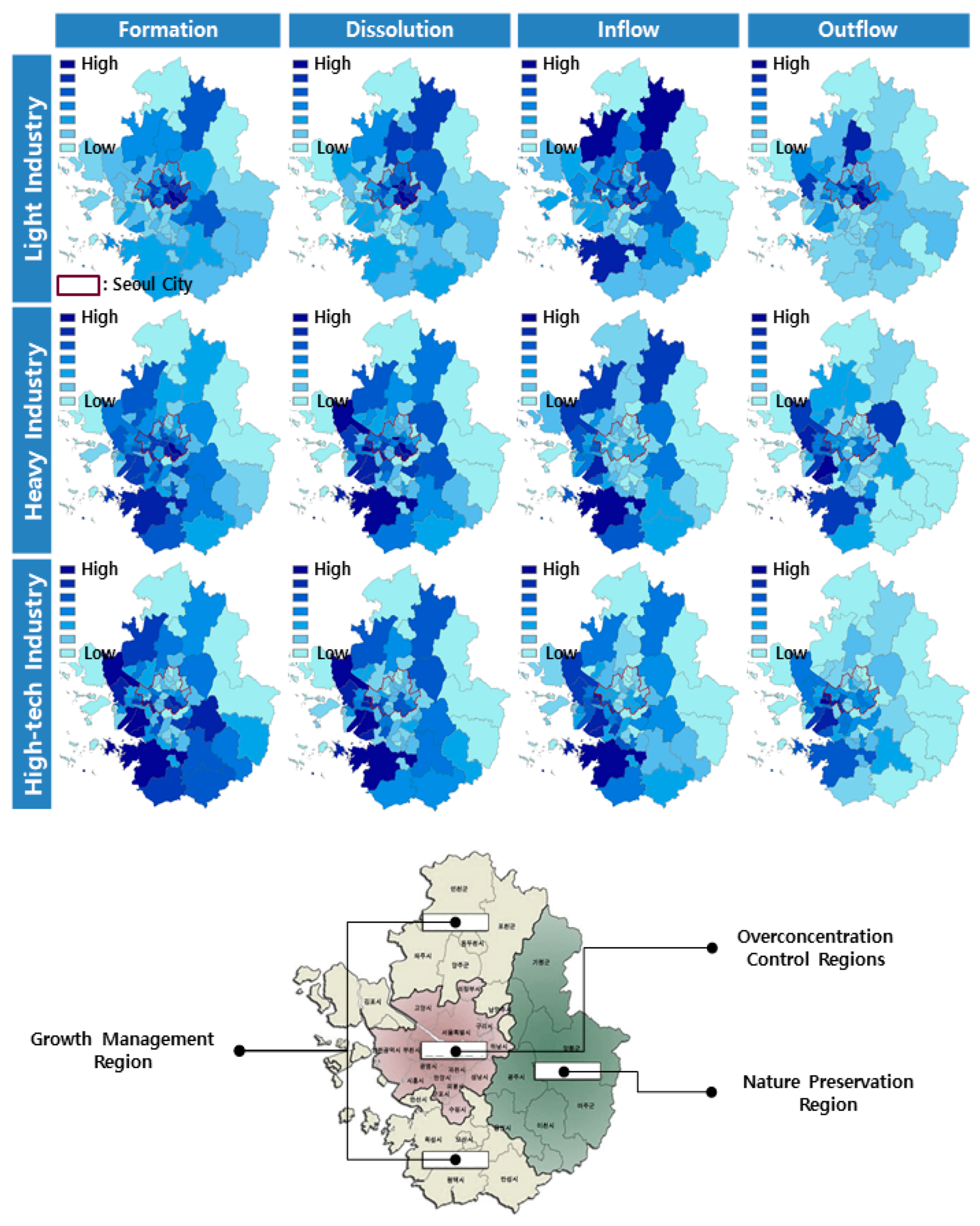
We provide the descriptive statistics of the aggregated city-level firm dataset in Table 2 and the city-level mappings in Figure 2. From Table 2, on average, cities tend to have a larger number of new than closed firms for all industry types except the light industry. In terms of absolute numbers, the high-tech industry had more new firm establishments and relocations than the other industry types.
In Figure 2, a similar spatial pattern is observed for both firm formation and dissolution for all industry types, implying that cities with high formation values usually have high dissolution values as well. The increasing competition incurred by new firms may contribute to this correlation. However, a different spatial pattern is observed for firm relocations. This empirical finding suggests that the relocation choices of firms may follow different mechanisms from the location choices of new firms. Specifically, the capital city of Seoul (center on the map) saw a significant outflow of light industry firms, which were relocated to the northern cities in SMA. Heavy and high-tech industry firms tend to relocate to the west coast area.
In addition, SMA is divided into three land-use regions (Overconcentration Control Regions, Growth Management Region, and Nature Preservation Region) under the Seoul Metropolitan Area Readjustment Planning Act. The Overconcentration Control Region (OCR) is defined as the area in which population and industries are, or are likely to be, excessively concentrated, so that decentralization is deemed necessary. The OCR covers the entire city of Seoul and its adjacent cities. The Growth Management Region (GMR) is designated to accommodate the population and industries relocated from the OCR through policy-oriented land-use development. The GMR applies to cities located in the northern and southern parts of SMA. Finally, the Nature Preservation Region, located in the eastern part of SMA, is proposed to preserve the natural environment, such as the Han River ecosystem and green belt of Seoul. [37].

4. Portfolio Analysis

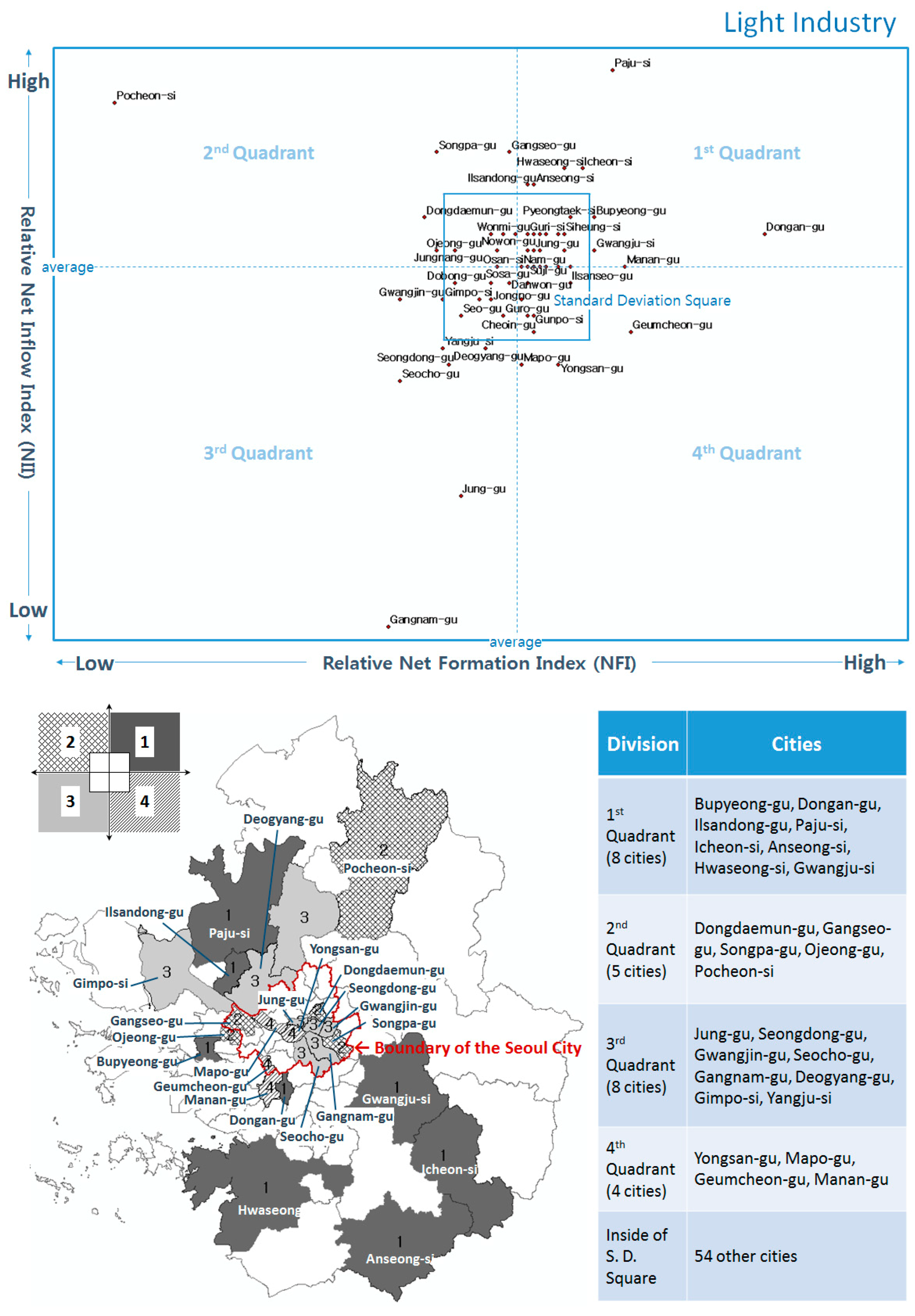
The results of the portfolio analysis for the light industry are shown in Figure 3. Eight cities are located in the first quadrant, which features relatively high values of NII and NFI. We thus posit that the light industry was growing in such cities during 2009–2010. Growth management policies may be required to prevent excess competition and environmental deterioration. In terms of location, these cities are mostly outside Seoul city, implying that central SMA is not a preferable location for light industry development, presumably due to high operation costs and stringent land-use controls.
In the second quadrant, a total of five cities are identified. Cities in the second quadrant have high NII values but low NFI values. On the one hand, the large inflow of light industry firms implies the attractiveness of the city; on the other hand, many existing local firms close, possibly because of the shock of the inflow firms. It is also possible that local firms merged with the inflow firms, thus disappearing from the registration record. In this case, the perceived number of “closed” firms may be biased. However, on average, the number of inflow firms is much lower than that of dissolution firms for all industry types (see Table 2). This implies that the mergers and acquisitions of local firms incurred by inflow firms may only account for a minor percentage. Nonetheless, we need to verify this potential bias once micro-level firm transaction data become available. Therefore, these cities may need policy incentives such as sector-specific subsidies or lending programs to support existing local firms.
The third quadrant represents the declining industry (low NFI and NII values). There are eight cities in this quadrant. In some case (e.g., Gangnam-gu, Jung-gu, and Seocho-gu in Seoul), the decline actually comes from policy-oriented restructuring of the local economy, where the light manufacturing industry was suppressed through policy interventions. For these cities, the loss of manufacturing jobs is likely to have significant impacts on the local supply chain as well as the communities. Policy initiatives should be considered to smooth the economic and social transition.
Finally, cities in the fourth quadrant can be interpreted as industry incubators (high NFI but low NII values). There are four cities in this quadrant, all of which are inside Seoul except for Manan-gu. In particular, Geumcheon-gu, as a well-developed industry area in Seoul, has the highest NFI value. On the one hand, the established infrastructure and proximity to the labor and consumer markets prompt new firms to locate in Seoul. On the other hand, many firms cannot withstand the increasing competition and high operation costs (e.g., high property rents), thus have to move to other cities.
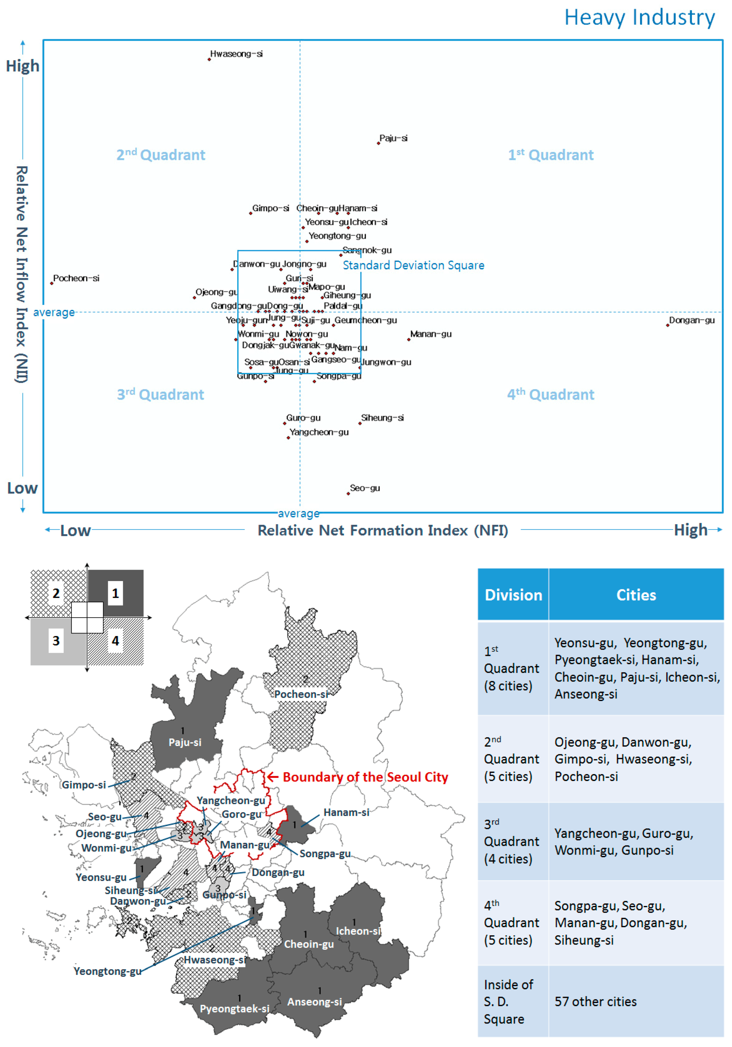
In terms of the heavy industry (see Figure 4), Paju-si had the highest values for both NFI and NII among the cities in the first quadrant, while the remaining cities are mainly in the southern areas of SMA. This is in line with the master plan of SMA—heavy industry is promoted in the southern areas of SMA, particularly along coastal cities. The five cities in the second quadrant feature high NII but low NFI values. Apart from Pocheon-si, all these cities are on the western coast of SMA. The high NII values come from the fact that this coast area has many ports, including an international harbor. Heavy industry firms tend to re-/locate close to the transport hubs. The four cities in the third quadrant are experiencing a declining heavy industry. These cities are mainly at Seoul’s periphery. Finally, there are five cities acting as incubators of the heavy industry. Note that high NFI values are present in Dongan-gu, Siheung-si, and Manan-gu, which are geographically contiguous. This implies that they are functioning as a cluster for heavy manufacturing industry.
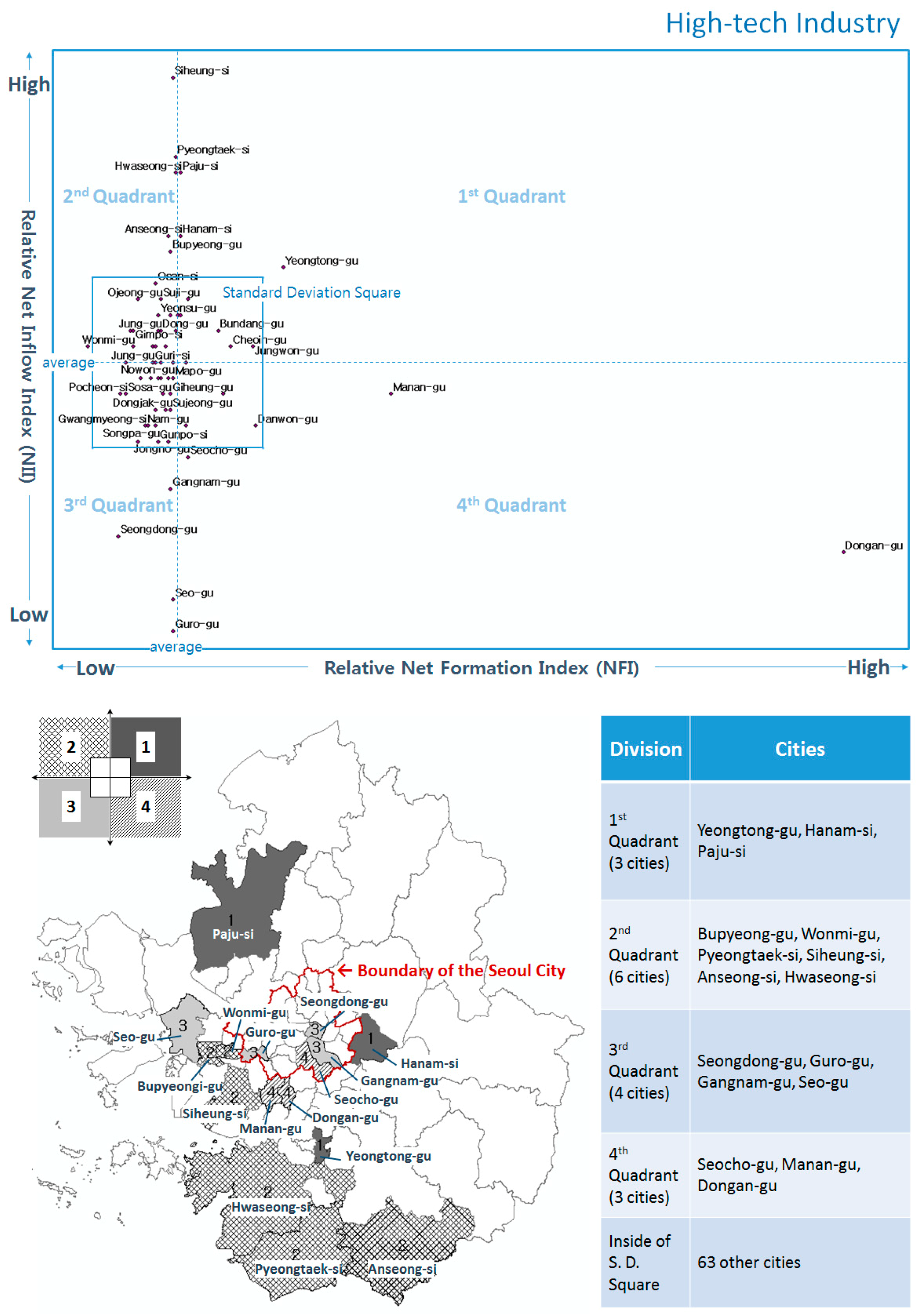
The high-tech industry presents different patterns (see Figure 5). Apart from Dongan-gu, the variance in NFI values across cities is small (i.e., cities are concentrated along the vertical axis rather than the horizontal). This suggests that the relocation of firms is a dominant feature for the high-tech industry, reflecting the relatively high mobility of high-tech firms. In this respect, the city sees the largest number of inflow firms is Siheung-si (second quadrant), followed by Pyeongtaek-si, Hwaseong-si, and Paju-si. By contrast, Guro-gu, Seo-gu, and Seongdong-gu present declining high-tech industries, with a considerable number of outflow firms. In addition, three incubator cities are identified for high-tech industry.
In sum, we make use of the proposed two industry indices, namely NFI and NII, to diagnose the city-level industry development in SMA. Different from traditional research, which largely focuses on the number of new or total firms, our portfolio analysis provides a more detailed study of the manufacturing industry in SMA cities. Specifically, for cities with high NFI and NII values (first quadrant) the manufacturing industry is believed to be growing. Typical cities are Paju-si and Dongan-gu for the light and heavy industries, and Yeongtong-gu and Hanam-si for the high-tech industry. By contrast, for cities with both low NFI and NII (third quadrant), a declining manufacturing industry is witnessed. Some cities of this type, such as Gangnam-gu, may undergo radical economic restructuring, but others may need particular policy attention to revive the local industry and employment. In addition, our analysis identifies cities potentially acting as industry incubators with high NFI and low NII values (fourth quadrant). The incubator function may represent a positive dynamic (i.e., new firms establish and then move out to other cities), but its economic sustainability is a question that local policy makers may need to deal with. In the presence of external shocks or periodic recessions, such cities may encounter a sharp industrial decline. In terms of the differences among industry types, the high-tech industry presents a much higher firm mobility than the other industries. In the next section, we present the regression analysis aiming to identifying the locational factors that may contribute to the observed patterns of industry development across SMA.

5. Regression Analysis

After the portfolio analysis, regression models are used aiming to identify city-level locational factors that contribute to the observed change patterns across cities in the SMA. The dependent variables are thus the zonal number of firms for each life-cycle change (i.e., formation, inflow, outflow, and closure). The independent variables are the city-level attributes. The selection of locational variables is informed by existing literature [24,27,33,34,35,40,41]. To address the issue of spatial autocorrelation and select the appropriate regression model accordingly, we follow established methods [43] based on empirical data. The regression analysis including the model selection process is presented in this section.

5.1. Setting Independent Variables

Based on the results of literature review, we divided the location factors of a large number of new firms, closed firms, inflowed firms, and outflowed firms into six categories: ‘Density Variables’, ‘Human Capital’, ‘Economic Variables’, ‘Floorspace’, ‘Location Quotient’, and ‘Transport’. The independent variables used in this study consist of 27 variables (see Table 3).
‘Density Variables’ is related to the market scale. This category includes not only population and employment but also the density of firms in the same industry [24,27,33,35]. ‘Human Capital’ ensures that the level of education required for each type of manufacturing industry is different and has an effect on it [24,27,44,45]. It shows the skill and education level of the local workforce. The economic level of a city (‘Economic Variable’) affects the city’s industrial structure and confirms that the larger the economy, the more advanced is the high-tech industry [24,33,44]. ‘Economic Variables’ represents the gross regional domestic product (GRDP), average land price, and the average floorspace rent for housing, industrial, and office use, respectively. ‘Floorspace’ determines how much floorspace in practice is available to firms or employees in the city [35,46,47]. In addition, ’Floorspace’ is also an important variable because this relates to a direct and practical industrial policy such as the development of industrial parks. ‘Floorspace’ consists of the total amount of floorspace and vacant floorspace available for housing, industrial, and office use, respectively. Through ‘Location Quotient’, we are expected to see how regional specialties in an industry affect the life cycle of the firm [24,33,43]. It also checks the agglomeration effect, which means checking the impact of the agglomeration of population, employment, and firms on the number of new firms, closed firms, and flowed in and flowed out firms in the city [11,24,27,33,35,41]. ‘Location Quotient’ measures the level of specialization of firms in one location relative to the regional average. ‘Transport’, is generally known to be a very important factor for a firm’s location [24,27,34,44,47,48]. Therefore, we focused on the fact that transportation facilities can affect closed firms and the outflow of the firms. In terms of ‘Transport’, we calculate the density of subway lines, road areas, and harbors.
In the next sections, we first present a baseline Ordinary Least Squares (OLS) regression model without considering the possible spatial autocorrelation. The spatial dependence issue is then investigated through a series of statistics tests following the method proposed by Anselin [43], which informs the selection of regression model for each change type of firms. The regression results are presented subsequently.

5.2. Fit a Baseline OLS Model without Considering Spatial Autocorrelation

Given the relatively large number of independent variables (27 variables in our case), defining a proper regression model could be an analytical challenge. We make use of the Exploratory Regression tool in the ArcGIS software to search for a best-fit model. The Exploratory Regression toolbox evaluates all possible combinations of the explanatory variables subject to a range of model performance diagnostics, e.g., R2, Variance Inflation Factor (VIF), Akaike Information Criterion (AIC), and Jarque-Bera p-values (JB) [49]. A maximum of five variables are allowed for the Explorative Regression. The results are verified through the stepwise variable selection method [50] by checking the change of model diagnostics after adding/deleting variables to the best-fit model.
The selected regression models and the diagnostics including the global Moran’s I statistics for spatial autocorrelation [28,38] are presented in Table 4. Note that the spatial matrix used in the Moran’s I test is the inverse distance between cities.

5.3. Diagnostics for Spatial Dependence

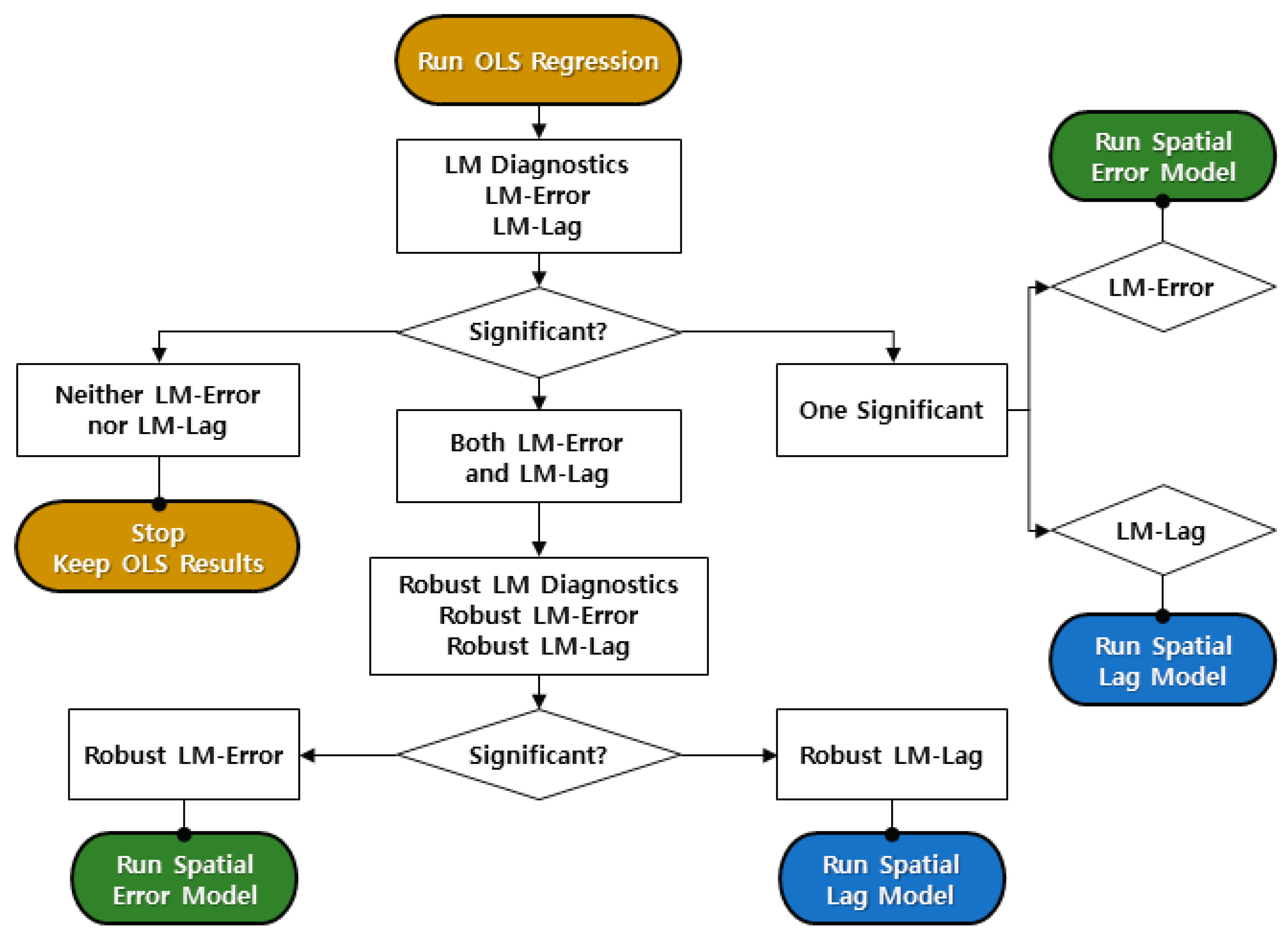
We tested the spatial dependence for the baseline OLS model using Lagrange Multiplier (LM) as in Anselin [43]. If there is spatial dependence between the variables in an OLS model, the model should be reanalyzed using a spatial regression model. The detailed process is as follows:
Initiate the process at the top of the graph and consider the standard (i.e., not the robust forms) LM-Error and LM-Lag test statistics. If neither rejects the null hypothesis, stick with the OLS results. It is likely that, in this case, the Moran’s I test statistic will not reject the null hypothesis either. If one of the LM test statistics rejects the null hypothesis, and the other does not, then the decision is also straightforward: Estimate the alternative spatial regression model that matches the test statistic that rejects the null. Thus, if LM-Error rejects the null, but LM-Lag does not, estimate a SEM, and vice versa. When both LM test statistics reject the null hypothesis, proceed to the bottom part of the graph and consider the robust forms of the test statistics. Typically, either only one of them will be significant (as in Figure 6) or one will be orders of magnitude more significant than is the other (e.g., p < 0.00000 compared to p < 0.03). In that case, the decision is simple: Estimate the spatial regression model matching the most significant statistic [39,43].
Table 5 shows the results of a diagnostic test for spatial dependence. Moreover, the inverse distance for each zone was used as the spatial weight matrix. The spatial dependence was checked only at the four models for Heavy Industry and High-tech Industry. Therefore, we analyzed the SEM for the New firms and the Closed firms models of both Heavy Industry and High-tech Industry. The SLM applied only to the Flowed out firms model of Heavy Industry. For others, we analyzed the OLS model.

5.4. Results of Regression Analysis

A summary of the OLS, SEM, and SLM regression results is provided in Table 6, Table 7 and Table 8. Overall, the R-squared values for all industry types are satisfactory, within the range of 0.56 and 0.86. We discuss the spatial regression results for the light, heavy, and high-tech industries in turn.

5.4.1. Light Industry

Table 6 reports the results for light industry. The variables ‘GRDP’ and ‘Dis2Har’ are significant for all models in light industry, which is in line with the literature [43,46,47]. However, the coefficient of GRDP is higher in ‘Closed Firms’ than in ‘New Firms’ and higher in ‘Inflow Firms’ than in ‘Outflow Firms’. We argue that, on the one hand, a high GRDP may imply a regional economic center where firms are attracted from other cities; on the other hand, competition among firms in high-GRDP cities is generally stronger, thus leading to more frequent changes of local firms. This is an advanced result of the study that shows that the city’s economic scale is positive for the increase in the number of the firms [51], indicating that there may be a decline in the number of the manufacturing firms due to an increase in the economic scale.
In terms of the Human Capital variables, ‘Ter_Deg’ is negatively correlated to ‘New Firms’ and ‘Wage’ is positively correlated to the Inflow Firms. This result shows that a higher income level is an important factor in relocation to the city. The coefficient of ‘LQ_light’ is significant in Inflow Firms, which suggests that light industry firms tend to concentrate in space through relocation. ‘FS_Vacan_Ind’ is negatively correlated with the Outflow Firms. It suggests that the undersupply of industrial floorspace and the resulting high property rent may cause light industry firms to flee. In addition, this is the outcome that corresponds to the findings of the studies that show that the availability of more land (or floor area) is positive for the position of the entity [52,53,54]. They also indicate that not only the increase in the available area but also the decrease in the number of vacant lots is important. This suggests that as the vacant industrial floorspace decreases, many light industry firms in the city outflow due to the increased competition for location; however, the coefficient in this regard is very low.

5.4.2. Heavy Industry

The results for heavy industry are presented in Table 7. Due to significant spatial dependence, Spatial Error model is applied for the New Firms and Close Firms, and Spatial Lag model is applied for the Inflow Firms. The Lambda (λ) and Rho (ρ) values are significant and have negative coefficients. which is in line with the negative Global Moran’s Index.
In terms of Floorspace variables, the FS_Ind variable is significant for Inflow Firms and the FS_Vacan_Ind is significant for New Firms, both with high t-value. It suggests that for new firms, the availability of industrial floorspace is likely to be an important locational factor, while for relocated firms, the size of the existing industrial floorspace stock matters. This indicates that the inflow of heavy industry firms is rather negative with regard to the result of the study [54,55], implying that the office floorspace is positive only for the inflow of service firms.
The density of heavy industry firms plays a significant role for the New Firms, the Inflow Firms and Outflow Firms. We argue that this reflects the dual effect of the agglomeration economy—the self-sustaining force of spatial concentration versus the negative externalities derived from overcrowding. This result is an improvement upon the study [41] that revealed that there is an agglomeration effect on the location determination of the manufacturing firms in the SMA. Lastly, as the distance from an international harbor is less, many heavy industry firms in the city outflow, signifying a competition for location. This is the same result as of the study [56].

5.4.3. High-Tech Industry

Table 8 presents the results for high-tech industry. SEM is applied for the Close Firms to address the spatial dependence issue. New high-tech firms tend to favor cities with quality housing [24], abundant industry floorspace, and high level of industry specialization. In fact, the location quotient variable (LQ_high-tech) is significant among all firm change models for high-tech industry, which is in line with the literature [57]. This suggests that, as opposed to the heavy and light industry, industry specialization is more important for understanding the locational choice of high-tech firms in SMA.
The housing rent is positively correlated to the New Firms, indicating that good quality of housing may attract high-tech firms. The employment density plays a significant role for Inflow Firms, which suggests that high-tech firms in SMA prefer established urban areas for relocation.

6. Conclusions

This paper presents an empirical study of spatial changes of manufacturing firms in the Seoul Metropolitan Area. The proposed method combines the conventional spatial analysis of firm location choices and the life-cycle perspective of firm development. Specifically, we combined the descriptive portfolio analysis with the spatial regression. The portfolio analysis decomposes the aggregate change of firms into four life-cycle types through a readily understandable interface. The subsequent spatial regression analysis examines the spatial change of firms in relation to various locational factors at the city-level. The combined approach provides a new strategy for diagnosing industry development across a cluster of inter-connected cities.
The portfolio analysis using net formation and net inflow Index provides a diagrammatic overview of cities in terms of their manufacturing development. Distinct development patterns have been visually identified. We deem that, compared against existing studies based on total number of (new) firms, the incorporation of life-cycle perspective, and the application of portfolio analysis is more informative. After the portfolio analysis, spatial regression models were tested and applied to identify the significant locational factors that contribute to the observed firm change patterns. The results show that different industry types may be affected by different locational factors. In particular, the agglomeration economy derived from the spatial proximity of similar firms is an important locational factor for high-tech firms in SMA. The dual effect of industrial specialization is identified. On the one hand, high level specialization attracts new or inflow firms. On the other hand, it leads to an increased number of closed or outflow firms, plausibly due to increased competition among local firms. We also find that the floorspace stock size and availability are significant factors for manufacturing firms in SMA.
One notable limitation associated with the regression exercise is that the explanatory variables selected remain rather aggregate in nature, which causes difficulty in interpreting regression results. The correlations identified need to be verified and clarified at a finer spatial scale, possibly with more targeted variable selection, when disaggregate data sources become available, so that causal relationships between the life-cycle changes of firms and the locational factors can be derived. Another limitation concerns the interplay between the light, heavy, and high-tech manufacturing firms—the spatial change of these firms may be inter-connected due to shared supply chain or location-specific policy interventions. The interdependence in life-cycle changes of firms is not considered in the paper. Finally, the current data set only covers 2009 to 2010—an expanded panel data set would help address short-term fluctuations and uncertainties.

Author Contributions

Y.A. and L.W. contributed equally to this work. Y.A. conceived the idea and analyzed it. L.W. wrote the manuscript and the discussion. All authors discussed the results and commented on the manuscript.

Funding

This work was supported by the Ministry of Education of the Republic of Korea and the National Research Foundation of Korea (NRF-2017S1A5A8021229 and 2017R1A2B4003949).

Acknowledgments

The authors also appreciate the support from the “Digital Cities for Change (DC2)” project at the Cambridge Centre for Smart Infrastructure and Construction, University of Cambridge. The DC2 project is funded by The Ove Arup Foundation.

Conflicts of Interest

The authors declare no conflicts of interest. The funders had no role in the design of the study; in the collection, analyses, or interpretation of data; in the writing of the manuscript, or in the decision to publish the results.

References

  1. Wegener, M. Operational urban models: State of the art. J. Am. Plan. Assoc. 1994, 60, 17–29. [Google Scholar] [CrossRef]
  2. Hyter, R. The Dynamics of Industrial Location: The Factory, the Firm and Production System; Department of Geography, Simon Fraser University: Burnaby, BC, Canada, 2004. [Google Scholar]
  3. Korean Statistical Information Service. 2016. Available online: http://kosis.kr/ (accessed on 5 February 2018).
  4. Lee, S.; An, Y.; Kim, K. Relationship between transit modal split and intra-city trip ratio by car for compact city planning of municipalities in the Seoul Metropolitan Area. Cities 2017, 70, 11–21. [Google Scholar] [CrossRef]
  5. Arauzo-Carod, J.; Liviano-Solis, D.; Manjón-Antolín, M. Empirical studies in industrial location: An assessment of their methods and results. J. Reg. Sci. 2010, 50, 685–711. [Google Scholar] [CrossRef]
  6. Artz, G.M.; Kim, Y.; Orazem, P.F. Does Agglomeration Matter Everywhere? New firm location decisions in rural and urban markets. J. Reg. Sci. 2016, 56, 72–95. [Google Scholar] [CrossRef]
  7. Sivakumar, A.; Bhat, C. Comprehensive, unified framework for analyzing spatial location choice. Transp. Res. Rec. 2007, 2003, 103–111. [Google Scholar] [CrossRef]
  8. Li, C.; Song, Y.; Chen, Y. Infrastructure Development and Urbanization in China. In China’s Urbanization and Socioeconomic Impact; Springer: Singapore, 2017; pp. 91–107. [Google Scholar]
  9. De Bok, M. Using firmographic microsimulation for land use and transport scenario valuation: Model calibration. In Proceedings of the 45th ERSA Congress, Amsterdam, The Netherlands, 23–27 August 2005; pp. 1–26. [Google Scholar]
  10. Alanón, A.; Arauzo, J.M.; Myro, R. Accessibility, agglomeration and location. Entrep. Ind. Locat. Econ. Growth 2007, 247–267. [Google Scholar]
  11. Arauzo-Carod, J.-M.; Viladecans, E. Industrial location at the intra-metropolitan level: The role of agglomeration economies. Reg. Stud. 2009, 43, 545–558. [Google Scholar] [CrossRef]
  12. Bhat, C.R.; Paleti, R.; Singh, P. A Spatial multivariate count model for firm location decisions. J. Reg. Sci. 2014, 54, 462–502. [Google Scholar] [CrossRef]
  13. Buczkowska, S.; de Lapparent, M. Location choices of newly created establishments: Spatial patterns at the aggregate level. Reg. Sci. Urban Econ. 2014, 48, 68–81. [Google Scholar] [CrossRef] [Green Version]
  14. Pellenbarg, P.H.; van Wissen, L.J.G.; van Dijk, J. Firm Relocation: State of the Art and Research Prospects; University of Groningen: Groningen, The Netherlands, 2002. [Google Scholar]
  15. Lee, B. A study on the determinants of manufacturing productivity. Korea Econ. Rev. 2000, 48, 291–322. [Google Scholar]
  16. Keeble, D.; Wever, E. New Firms and Regional Development in Europe; Taylor & Francis: Milton Park, UK, 1986. [Google Scholar]
  17. Papke, L.E. Interstate business tax differentials and new firm location: Evidence from panel data. J. Public Econ. 1991, 45, 47–68. [Google Scholar] [CrossRef]
  18. Wang, F.; Chen, C.; Xiu, C.; Zhang, P. Location analysis of retail stores in Changchun, China: A street centrality perspective. Cities 2014, 41, 54–63. [Google Scholar] [CrossRef]
  19. Fahmi, F.Z.; Koster, S.; van Dijk, J. The location of creative industries in a developing country: The case of Indonesia. Cities 2016, 59, 66–79. [Google Scholar] [CrossRef]
  20. Musil, R.; Eder, J. Towards a location sensitive R&D policy. Local buzz, spatial concentration and specialisation as a challenge for urban planning—Empirical findings from the life sciences and ICT clusters in Vienna. Cities 2016, 59, 20–29. [Google Scholar] [CrossRef]
  21. Moeckel, R. Microsimulation of firm location decisions. In Proceedings of the 9th International Conference on Computers in Urban Planning and Urban Management, London, UK, 7 June 2005; pp. 2005–2029. [Google Scholar]
  22. Van Wissen, L. A micro-simulation model of firms: Applications of concepts of the demography of the firm. Pap. Reg. Sci. 2000, 79, 111–134. [Google Scholar] [CrossRef]
  23. Van Wissen, L. Demography of the firm: A useful metaphor? Eur. J. Pop. 2002, 18, 263–279. [Google Scholar] [CrossRef]
  24. An, Y.; Kang, Y.; Lee, S. A study on the impact of soft location factors in the relocation of service and manufacturing firms. Int. J. Urban Sci. 2014, 18, 327–339. [Google Scholar] [CrossRef]
  25. Van Wissen, L. The Concept of Carrying Capacity in the Demography of Firms. In Population and Families in the Low Countries; van den Brekel, H., Deven, F., Eds.; Kluwer Academic Publishers: Dordrecht, The Netherlands, 1997; pp. 219–244. [Google Scholar]
  26. Van Dijk, J.; Pellenbarg, P.H. Firm relocation decisions in The Netherlands: An ordered logit approach. Pap. Reg. Sci. 2000, 79, 191–219. [Google Scholar] [CrossRef]
  27. Chin, A.; Hong, J. The Location Decisions of Foreign Logistics Firms in China: Does Transport Network Capacity Matter? East Asian Bureau of Economic Research: Canberra, Australia, 2005. [Google Scholar]
  28. Koenig, W.D.; Knops, J.M.H. Testing for spatial autocorrelation in ecological studies. Ecography 1998, 21, 423–429. [Google Scholar] [CrossRef]
  29. Koenig, W.D. Spatial autocorrelation of ecological phenomena. Trends Ecol. Evol. 1999, 14, 22–26. [Google Scholar] [CrossRef]
  30. Anselin, L. Local indicators of spatial association—LISA. Geogr. Anal. 1995, 27, 93–115. [Google Scholar] [CrossRef]
  31. Smith, T.E. Notebook on Spatial Data Analysis. 2016. Available online: http://www.seas.upenn.edu/~ese502/#notebook (accessed on 25 February 2018).
  32. Michael, D.W.; Kristian, S.G. Spatial Regression Models; SAGE Publications, Inc.: Thousand Oaks, CA, USA, 2008. [Google Scholar]
  33. Woodward, D.P. Locational determinants of Japanese manufacturing start-ups in the United States. South. Econ. J. 1992, 58, 690–708. [Google Scholar] [CrossRef]
  34. Cheng, L.K.; Kwan, Y.K. What are the determinants of the location of foreign direct investment? The Chinese experience. J. Int. Econ. 2000, 51, 379–400. [Google Scholar] [CrossRef]
  35. Lee, H.; Lee, B. An analysis of firm relocation in the manufacturing industries. J. Korea Plan. Assoc. 2002, 37, 103–116. [Google Scholar]
  36. Korea Chamber Commerce and Industry (KCCI). Available online: http://www.korcham.net/ (accessed on 5 February 2018).
  37. The National Law Information Center, the Korea Representative Legal Information Web Site. Available online: http://www.law.go.kr/ (accessed on 5 February 2018).
  38. Hurlbert, S.H. Pseudoreplication and the design of ecological field experiments. Ecol. Monogr. 1984, 54, 187–211. [Google Scholar] [CrossRef]
  39. Stephen, A.M. GeoDa and Spatial Regression Modelling; Population Research Institute: Front Royal, VA, USA, 2006. [Google Scholar]
  40. Yi, C. An Analysis on the Determinants of the Agglomeration by Industrial Type in Seoul Metropolitan Region with Spatial Econometrics. Gyeonggi Res. Inst. 2016, 16, 1–33. [Google Scholar]
  41. An, Y.; Wan, L. Modelling industrial firm relocation with impacts of spatial dependence. Int. J. Urban Sci. 2018, 22, 80–103. [Google Scholar] [CrossRef]
  42. Korea Chamber Commerce and Industry. Business Yearbook. Maeil Business News Korea, 2009 and 2010.
  43. Anselin, L. Exploring Spatial Data with GeoDaTM: A Workbook; Center for Spatially Integrated Social Science: Santa Barbara, CA, USA, 2005. [Google Scholar]
  44. Bartik, T.J. Business location decisions in the United States: Estimates of the effects of unionization, taxes, and other characteristics of states. J. Bus. Econ. Stat. 1985, 3, 14–22. [Google Scholar]
  45. Agarwal, R.; Audretsch, D.B. Does entry size matter? The impact of the life cycle and technology on firm survival. J. Ind. Econ. 2001, 49, 21–43. [Google Scholar] [CrossRef]
  46. Henderson, V.; Kuncoro, A.; Turner, M. Industrial development in cities. J. Political Econ. 1995, 103, 1067–1090. [Google Scholar] [CrossRef]
  47. Do, H.; Lee, Y. Empirical study on firm relocation choice in Seoul metropolitan area. Seoul Stud. 2008, 9, 131–144. [Google Scholar]
  48. Erickson, R.A.; Wasylenko, M. Firm relocation and site selection in suburban municipalities. J. Urban Econ. 1980, 8, 69–85. [Google Scholar] [CrossRef]
  49. Braun, M.T.; Oswald, F.L. Exploratory regression analysis: A tool for selecting models and determining predictor importance. Behav. Res. Methods 2011, 43, 331–339. [Google Scholar] [CrossRef]
  50. Choi, U.; Kwon, O.; Lee, E.; Son, D.; Cho, M.; Chung, Y. Evaluating of Sigumajang Aroma by Stepwise Multiple Regression Analysis of Gas Chromatographic Profiles. J. Microbiol. Biotechnol. 2000, 10, 476–481. [Google Scholar]
  51. Rubalcaba, L.; Michel, S.; Sundbo, J.; Brown, S.W.; Reynoso, J. Shaping, organizing, and rethinking service innovation: A multidimensional framework. J. Serv. Manag. 2012, 23, 696–715. [Google Scholar] [CrossRef]
  52. Heckman, J.S. Survey of Location Decisions in The South. Econ. Rev. 1982, 6, 6–19. [Google Scholar]
  53. Oum, T.H.; Park, J.H. Multinational firms’ location preference for regional distribution centers: Focus on the Northeast Asian region. Transp. Res. Part E Logist. Transp. Rev. 2004, 40, 101–121. [Google Scholar] [CrossRef]
  54. Yan, J. A Study on the Changing Location of Office Space in Seoul Metropolitan Area; Seoul Institute: Seoul, Korea, 2004. [Google Scholar]
  55. Choi, J.Y.; Oh, K.S. An Analysis of Relocation of SW Industries using GIS Flow Map. J. Korea Spat. Inf. Soc. 2010, 18, 41–52. [Google Scholar]
  56. Hong, S. Choice of Location Regarding to the Type of Business and the Trait of Regions; Yonsei University: Seoul, Korea, 2006. [Google Scholar]
  57. Wan, L.; An, Y. Identifying growth patterns of the high-tech manufacturing industry across the Seoul metropolitan area using latent class analysis. J. Urban Plan. Dev. 2017, 143, 04017011. [Google Scholar] [CrossRef]
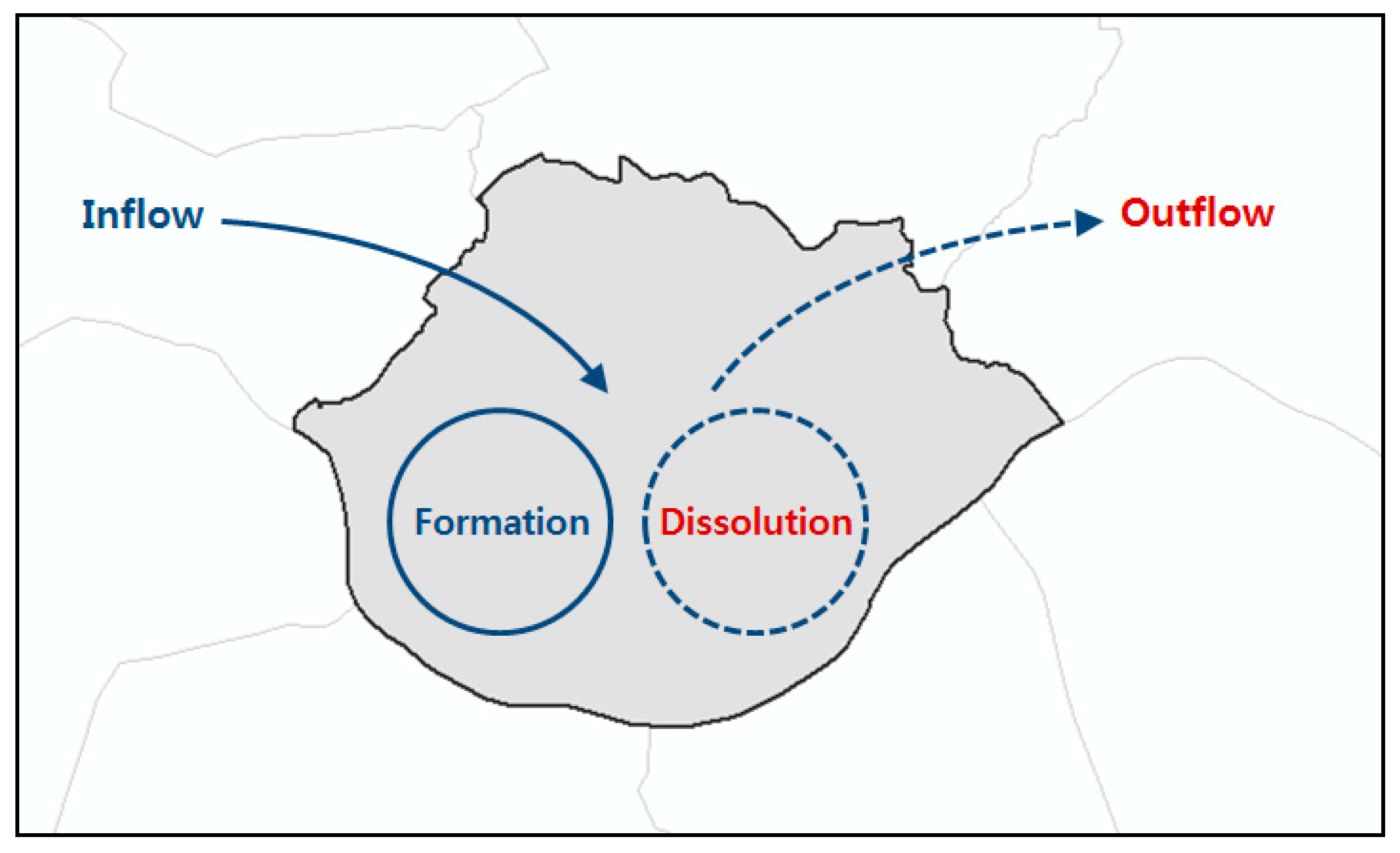
Figure 1. Change in the of number of firms in a region divided into four types.
Sustainability 11 03808 g001
Figure 2. Spatial pattern of firm life-cycle changes and regional land-use scheme in SMA.
Sustainability 11 03808 g002
Figure 3. Portfolio analysis for the light industry.
Sustainability 11 03808 g003
Figure 4. Portfolio analysis for the heavy industry.
Sustainability 11 03808 g004
Figure 5. Portfolio analysis for the high-tech industry.
Sustainability 11 03808 g005
Figure 6. Spatial regression decision process [40,43].
Sustainability 11 03808 g006
Table 1. Basic statistics of spatial changes of manufacturing firms in the Seoul Metropolitan Area (SMA).
Industry TypeTotal Firms *** (2010)New Firms (2010)Closure Firms (2010)Relocated Firms (2009–2010)
Total RelocationIntra-City * RelocationInter-City ** Relocation
No.RatioNo.RatioNo.RatioNo.RatioNo.Ratio
Light Industry10,596187717.7%209719.8%123211.6%8888.4%3443.2%
Heavy Industry14,994275518.4%267517.8%13729.2%9836.4%3892.6%
High-Tech Industry15,788341021.6%271112.2%204613.0%14689.3%5783.7%
Total41,378804219.4%748318.1%465011.2%33398.1%13113.2%
* Intra-city relocation means the relocation origin and destination are in the same cities in SMA. ** Inter-city relocation means the relocation origin and destination are in different cities in SMA. *** Total number of firms in 2010 includes existing firms from 2009 plus new firms, minus closure firms.
Table 2. Variables related to the firm-life cycle (aggregated across 78 cities).
DivisionVariableNAvg.SumMin.Max.S. d.
Light IndustryFormation F l i g h t f o r 7923.81877011322.0
Dissolution F l i g h t d i s 7926.52097013226.8
RelocationInflow F l i g h t i n 794.43440204.3
Outflow F l i g h t o u t 794.43440426.5
Heavy IndustryFormation F h e a v y f o r 7934.92755126343.5
Dissolution F h e a v y d i s 7933.92675028644.6
RelocationInflow F h e a v y i n 794.93890366.0
Outflow F h e a v y o u t 794.93890325.7
High-tech IndustryFormation F h i g h t e c h f o r 7943.23410034359.0
Dissolution F h i g h t e c h d i s 7934.32711025844.1
RelocationInflow F h i g h t e c h i n 797.325780447.9
Outflow F h i g h t e c h o u t 797.325780358.1
Table 3. List of independent variables and the sources.
Type of VariablesMarksDefinitionSourcesYearDescriptive Statistics
Min.Max.MeanStd. Dev. Dev.
Density VariablesPop_DenResidential population (10,000 persons) per km2KOSIS *2010456.927,578.19572.87131.9
Emp_DenNumber of existing employees (10,000 persons) per km2KOSIS2010146.016,724.13854.43638.6
Firm_DenNumber of existing manufacturing firms per km2KOSIS201038.22311.0695.1558.8
L_Firm_DenNumber of existing light industry firms per km2KOSIS20100.3363.228.347.2
H_Firm_DenNumber of existing heavy industry firms per km2KOSIS20101.1194.527.034.9
T_Firm_DenNumber of existing high-tech industry firms per km2KOSIS20100.0258.416.835.9
Human CapitalSec_DegPercentage of working persons with high school degreeKOSIS20100.10.40.30.0
Ter_DegPercentage of working persons with bachelor’s degree or higherKOSIS20100.00.10.00.0
WageAverage wage per household (1–10, 10: high, 1: low)Biz-GIS **20101.77.13.61.0
Economic VariablesGRDPTotal amount of GRDP (100 million won)KOSIS201039.8163890.731679.497604.829
Land_PLand price (1 million won) per m2Official Data2010618.875,591.116,885.615,710.2
FS_R_HSRent fee of residential floorspace (10,000 won) per m2Official Data20100.11.80.90.4
FS_R_IndRent fee of industrial floorspace (10,000 won) per m2Official Data20101.01.91.20.2
FS_R_OffRent fee of official floorspace (10,000 won) per m2Official Data20102.46.73.40.9
FloorspaceFS_HSTotal amount of residential floorspace (km2)KOSIS20100.5637843.0706011.100360.788842
FS_IndTotal amount of industrial floorspace (km2)KOSIS20100.1123614.290202.107152.81322
FS_OffTotal amount of office floorspace (km2)KOSIS20100.0995111.498201.334401,079,954
FS_Vacan_HSTotal amount of vacant residential floorspace (m2)KOSIS201051,1112,888,580495,886476,905
FS_Vacan_IndTotal amount of vacant industrial floorspace (m2)KOSIS201076401,228,960187,815254,909
FS_Vacan_OffTotal amount of vacant office floorspace (m2)KOSIS201012,936655,39798,564110,519
Location QuotientLQ_lightLocation quotient of light industryKOSIS20100.14.81.01.1
LQ_heavyLocation quotient of heavy industryKOSIS20100.00.20.00.0
LQ_highLocation quotient of high-tech industryKOSIS20100.00.20.00.0
LQ_allLocation quotient of all industryKOSIS20100.13.21.00.8
TransportSub_DenNumber of subway stations per km2NGII ***20100.00.90.20.2
Road_RatioLength of road in km2NGII20100.00.20.10.1
Dis2HarDistance to an international harbor from center point each city (km)NGII20108.511.410.40.6
* KOSIS (Korea Statistical Information Service); ** Biz-GIS (http://www.biz-gis.com/); *** NGII (National Geographic Information Institute).
Table 4. Results of Exploratory Regression.
Industry TypeDependent VariableAdj. R2AICcJBK (BP)VIFMoran’s I (p-Value)Model
LightNew firms0.77599.620.000.502.660.0199
(0.50)
− Ter_Deg *** + GRDP ***
+ FS_R_Ind *** + Dis2Har ***
+ LQ_all ***
Closed firms0.79621.720.440.001.72−0.0328
(0.69)
+ Sec_Deg + GRDP *** + Dis2Har *** + LQ_light *** + LQ_all ***
Flowed in firms0.60388.710.050.001.15−0.0103
(0.96)
+ Pop_Den + Wage *** + GRDP ***
+ Dis2Har *** + LQ_light **
Flowed out firms0.78404.780.110.002.010.0254
(0.44)
+ Sec_Deg ** + GRDP ***
+ Dis2Har ***
− FS_Vacan_Ind *** + LQ_all ***
HeavyNew firms0.77703.510.000.013.05−0.1060
(0.05)
+ H_Firm_Den *** + GRDP ***
+ FS_R_HS **
+ FS_Vacan_Ind *** + LQ_heavy
Closed firms0.84680.840.000.002.49−0.1015
(0.06)
+ GRDP *** + FS_HS ***
− FS_Vacan_HS ***
+FS_Vacan_Ind **+LQ_heavy ***
Flowed in firms0.76396.810.000.003.98−0.0976
(0.08)
+ H_Firm_Den *** + GRDP ***
+ FS_Ind *** − FS_Vacan_Off
Flowed out firms0.65418.750.000.011.57−0.0319
(0.70)
+ Emp_Den *** + H_Firm_Den ***
− Dis2Har * + FS_Vacan_Ind ***
High-techNew firms0.53808.350.000.583.65−0.0259
(0.75)
+ FS_R_HS ** + FS_Ind ***
+ FS_Vacan_Off
+ LQ_high *** − LQ_all ***
Closed firms0.80694.700.000.002.53−0.0888
(0.12)
+ GRDP *** + FS_HS ***
+ FS_Ind *** − FS_Vacan_HS ***
+ LQ_high ***
Flowed in firms0.81426.140.080.003.44−0.0406
(0.58)
+ Emp_Den *** + FS_HS ***
+ FS_Ind ***
+ LQ_high *** − LQ_all ***
Flowed out firms0.62481.070.010.003.49−0.0407
(0.57)
+ Emp_Den + Land_P **
+ FS_Vacan_Ind ***
+ LQ_high *** − LQ_all ***
*: p-value < 0.1, **: p-value < 0.05, ***: p-value < 0.01.
Table 5. Results of diagnostic test for spatial dependence.
Industry TypeDependent VariableValuesLagrange MultiplierRobust LMDiagnostic
LagErrorLagError
LightNew firmsValue0.12640.01160.14590.0311OLS
p-value0.72220.91430.70250.8601
Closed firmsValue1.12441.49170.17000.5373OLS
p-value0.28900.22200.68010.4636
Flowed in firmsValue0.90660.50110.40610.0007OLS
p-value0.34100.47900.52390.9791
Flowed out firmsValue0.25670.01030.57290.3265OLS
p-value0.61240.91910.44910.5677
HeavyNew firmsValue4.53845.96320.95452.3794SEM
p-value0.03310.0146 **0.32860.1230
Closed firmsValue2.77675.43180.58383.2388SEM
p-value0.09570.0198 **0.44490.0719 *
Flowed in firmsValue4.81313.22291.99740.4071SLM
p-value0.0282 **0.0726 *0.15760.5234
Flowed out firmsValue0.35850.74350.01130.3963OLS
p-value0.54930.38850.91540.5290
High-techNew firmsValue1.98520.22692.45230.6940OLS
p-value0.15880.63380.11740.4048
Closed firmsValue0.12593.09610.29633.2664SEM
p-value0.72270.0785 *0.58620.0707 *
Flowed in firmsValue0.61050.14180.47240.0037OLS
p-value0.43460.70650.49190.9517
Flowed out firmsValue0.96180.42000.54340.0017OLS
p-value0.32670.46100.51690.9676
Table 6. Regression results for Light Industry.
Firm Life CycleIndependent VariableCoefficientt(z)-ValueModelMode Performance
Adj.R2
(R2)
Log
Likelihood
AIC
(SC)
New
Firms
Constant−149.07 ***−6.00OLS0.765896
(0.781097)
−292.009596.018
(610.158)
Ter_Deg−295.27 ***−3.53
GRDP2.5 × 10−6 ***8.17
FS_R_Ind37.49 ***3.47
Dis2Har10.17 ***4.58
LQ_all12.30 ***7.04
Close
Firms
Constant−143.49 ***−4.33OLS0.790968
(0.804542)
−303.061618.123
(632.263)
Sec_Deg66.33 *1.96
GRDP3.4 × 10−6 ***13.02
Dis2Har10.34 ***3.68
LQ_light_317.94 ***5.06
LQ_all7.16 ***2.98
Inflow
Firms
Constant−20.79 ***−3.40OLS0.598220
(0.624310)
−186.556385.111
(399.251)
Pop_Den8.5 × 10−5 *1.82
Wage0.93 **2.71
GRDP4.5 × 10−7 ***8.24
Dis2Har1.56 **2.70
LQ_light39.71 ***3.51
Outflow
Firms
Constant−26.95 ***−3.43OLS0.779076
(0.793422)
−194.592401.184
(415.324)
Sec_Deg16.61 *1.84
GRDP1.2 × 10−6 ***14.90
Dis2Har1.88 ***2.92
FS_Vacan_Ind−1.2 × 10⁻⁵ ***−6.20
LQ_all2.46 ***4.16
* p-value < 0.1, ** p-value < 0.05, *** p-value < 0.01.
Table 7. Regression results for Heavy Industry.
Firm Life CycleIndependent VariableCoefficient.t(z)-ValueModelMode Performance
Adj.R2
(R2)
Log
Likelihood
AIC
(SC)
New
Firms
Constant−33.13 ***−4.84SEM-
(0.813982)
−340.442692.883
(707.023)
H_Firm_Den0.18 ***3.02
GRDP1.5 × 10−6 ***3.28
FS_R_HS27.23 ***3.71
FS_Vacan_Ind1.1 × 10−4 ***8.52
LQ_heavy8.28 **2.44
Lambda (λ)−0.65 ***−3.30
Close
Firms
Constant−19.81 ***−5.57SEM-
(0.862736)
−329.962671.923
(686.064)
GRDP2.5 × 10−6 ***7.50
FS_HS1.3 × 10−6 ***3.63
FS_Vacan_HS−2.7 × 10⁻⁵ ***−4.57
FS_Vacan_Ind7.3 × 10−5 ***7.52
LQ_heavy22.19 ***8.80
Lambda (λ)−0.53 **−2.40
Inflow
Firms
Constant0.560.69SLM-
(0.784754)
−189.953391.906
(406.046)
H_Firm_Den0.04 ***5.03
GRDP3.8 × 10−7 ***3.65
FS_Ind1.3 × 10−6 ***9.64
FS_Vacan_Off−9.2 × 10⁻⁶ *−1.63
Rho (ρ)−0.23 **−1.76
Outflow
Firms
Constant13.60 *1.86OLS0.647335
(0.665655)
−202.783415.567
(427.351)
Emp_Den5.0 × 10−4 ***4.01
H_Firm_Den0.05 ***5.04
Dis2Har−1.30 *−1.88
FS_Vacan_Ind7.7 × 10−6 ***4.45
*: p-value < 0.1, **: p-value < 0.05, ***: p-value < 0.01.
Table 8. Regression results for the high-tech industry.
Firm Life CycleIndependent VariableCoefficientt(z)-ValueModelMode Performance
Adj.R2
(R2)
Log LikelihoodAIC
(SC)
New
Firms
Constant−26.20−1.40OLS0.529758
(0.560293)
−396.375804.75
(818.891)
FS_R_HS39.10 **2.13
FS_Ind1.1 × 10−5 ***4.99
FS_Vacan_Off7.6 × 10−51.49
LQ_high1089.08 ***5.07
LQ_all−34.54 ***−2.98
Close
Firms
Constant−15.75 **−2.62SEM-
(0.678434)
−361.471734.942
(749.083)
GRDP1.8 × 10−6 ***3.51
FS_HS2.9 × 10−6 ***5.02
FS_Ind6.9 × 10−6 ***4.57
FS_Vacan_HS−4.6 × 10⁻⁵ ***−4.97
LQ_high14.26 ***3.73
Lambda (λ)0.110.46
Inflow
Firms
Constant−0.52−0.57OLS0.806362
(0.818936)
−205.268422.537
(436.677)
Emp_Den6.3 × 10−5 ***5.50
FS_HS1.2 × 10−7 **2.34
FS_Ind1.7 × 10−6 ***9.25
LQ_high148.86 ***8.31
LQ_all−4.58 ***−4.71
Outflow
Firms
Constant−0.64−0.48OLS0.619042
(0.643780)
−232.734477.467
(491.608)
Emp_Den4.5 × 10−4 *1.70
Land_P1.6 × 10−6 **2.44
FS_Vacan_Ind1.5 × 10−5 ***4.81
LQ_high171.08 ***6.32
LQ_all−5.15 ***−3.70
* p-value < 0.1, ** p-value < 0.05, *** p-value < 0.01.