The Spatial-Temporal Characteristics of Cultivated Land and Its Influential Factors in The Low Hilly Region: A Case Study of Lishan Town, Hubei Province, China

Abstract

Cultivated land is a basic resource that is related to the sustainable development of the global economy and society. Studying the spatial and temporal distribution of cultivated land and its influential factors at the township scale is an important way to improve its sustainable use. Based on the land use data in 2009 and 2015, this paper comprehensively uses kernel density estimation, spatial autocorrelation analysis, and the spatial autoregressive model to analyze the spatial distribution characteristics and influential factors of cultivated land. The results show that in 2009 and 2015, the maximum kernel density of cultivated land in Lishan Town was 31/km² and 38/km², respectively, and there is an increasing tendency for it in the future. The global spatial autocorrelation Moran’s I of the proportion of cultivated land area in the administrative villages of Lishan Town in 2009 and 2015 was 0.5251 and 0.3970, respectively. Cultivated land has significant spatial self-positive correlation agglomeration characteristics in spatial distribution. Based on spatial error model (SEM) analysis, the regression coefficients of the village were 0.236 and 0.196 in 2009 and 2015, respectively. The regression coefficients of the road were 0.632 and 0.630, respectively. The regression coefficients of the water system were 0.481 and 0.290, respectively. The regression coefficients of the topographic position index were −0.817 and −0.672, respectively. By comparing 2015 with 2009, the regression coefficients of each influential factor have been reduced to varying degrees.

1. Introduction

Cultivated land resources are an important basis for the development of agricultural production and have great practical significance for safeguarding food security and social sustainable development [1]. Against a background of a continuously increasing world population, the reduction of per person cultivated land occupation and the enormous challenges of food security, it is of great importance to explore the quantity, spatial distribution and temporal and spatial characteristics of global cultivated land resources for strategic decision-making of food security internationalization [2]. According to the latest statistics of the Food and Agriculture Organization of the United Nations (FAO), the area of cultivated land in the world has increased from 1.279 billion hm² in 1961 to 1.730 billion hm² in 2015, and the total area of cultivated land has increased year by year. However, the area of cultivated land per person in the world was 0.415 hm² in 1961, and it was 0.265 hm² in 1990. By 2015, the area of cultivated land per person had decreased to a minimum of 0.26 hm². From 1961 to 2015, the cultivated land per person area decreased by 37.35% [3,4]. This was due to rapid population growth and the fact that human values change over time and that the production demands of humans cannot be achieved without the alteration or conversion of land use/cover (LULC) [5,6]. In addition, as an important type of artificial landscape, the expansion of cultivated land use, land reclamation, crop type replacement and conversion of other land types will change the material flow and energy flow of cultivated land [7], resulting in global changes with respect to climate, hydrology, and the biological earth cycle of the Earth system. Therefore, exploring the temporal and spatial changes of cultivated land also serves as the basis for studying the sustainable development of economic, social and ecological environment.

Insufficient area of cultivated land per person, low-quality cultivated land, and the continuous reduction of cultivated land reserve resources are the basic national conditions of China [8]. With the continuous increase of the population and the rapid development of the economy, the contradiction between the population and cultivated land has become more and more prominent. In recent years, due to the accelerating processes of industrialization and new urbanization in China, as well as the adjustment of internal structures of agriculture, the return of farmland to forests and grasslands, and the destruction caused by natural disasters, it is inevitable that the occupation and transformation of cultivated land resources will occur. The loss of a large number of high-quality cultivated land resources, and the difficulty of developing available reserve farmland resources have led to a continuous decline of the cultivated land resources in China. At the end of 2017, the area of cultivated land in China was 134.86 million km², but the construction area, disasters, ecological restoration, and adjustment of agricultural structure led to a small area of 3204 km². Under the influence of land remediation and agricultural restructuring, the area of cultivated land increased by 2595 km², which eventually led to a reduction of 609 km² of cultivated land during the year [9]. The shortage of cultivated land resources and its reserve resources are an indisputable fact. Therefore, the changing characteristics and spatial evolution of cultivated land have become an important part of land use/land cover change (LUCC) research.

In addition, the strategic position of the country’s ecological civilization construction has been upgraded, leading to the multiple pressures of quantity protection, quality management and the ecological restoration of cultivated land in China [10,11]. The “Opinions on Strengthening the Protection of Cultivated Land and Improving the Balance of Occupation and Compensation” issued by the Party Central Committee and the State Council and the report of the 19th National Congress of the Communist Party of China clearly require a strict observance of “the red line of cultivated land” and strengthen the quantity, quality and ecology of cultivated land [12,13]. This “Trinity” protection strives to form a new pattern of cultivated land protection with stronger protection, smoother implementation and more efficient management [14,15,16]. Strengthening the analysis of the spatial distribution of cultivated land and its influential factors to improve the sustainable use of cultivated land is an important way to alleviate the pressure on cultivated land protection.

At present, many scholars have carried out a large amount of theoretical research and practice on cultivated land resources and have obtained rich research results. In general, these studies mainly cover the spatial distribution patterns and morphological changes of cultivated land [17,18,19], the temporal and spatial evolution of the quality of cultivated land [17,20,21,22], ecological security evaluations of cultivated land [23,24,25], temporal and spatial changes of cultivated land [23,26,27,28], the prediction of cultivated land change [29,30], and the optimized layout of cultivated land [31,32,33]. The research areas of scholars have further expanded from the national, large-area, and provincial-level macro levels to the meso levels of cities and counties. In this research, traditional mathematical research methods, spatial data analyses and geostatistical methods are widely used [34,35,36]. At the same time, based on the theory of data restriction, some scholars have studied the spatial distribution characteristics of cultivated land resources in a specific historical period [37,38]. Data types are mainly based on high-resolution, high-precision land use/cover change data. However, there are still shortcomings in the following areas: most of the research on the spatial distribution of cultivated land resources is concentrated at the provincial and municipal levels, and there are few studies at the micro scale; and there is a lack of research on the dynamics of cultivated land resources and the extent of their impacts. In addition, although traditional linear regression analysis provides better ideas for solving this problem, it lacks a consideration of the interrelationship of research objects in a geospatial manner, especially for cultivated land, which has significant geospatial and social attributes. This issue may lead to deviations in the estimation results of the model.

For this reason, this paper is mainly based on the land use change of Lishan Town, Hubei Province, China, in 2009 and 2015, through the calculation of the kernel density value of the cultivated land and based on the global spatial autocorrelation of Moran’s I index and the local spatial autocorrelations of Moran’s I index of cultivated land are used to analyze the distribution characteristics of cultivated land resources. Then, the spatial autoregression model is introduced to compare and analyze the influence degree of each influential factor (elevation, slope, villages, roads, and water systems) of cultivated land. In addition, this article mainly studies the spatial-temporal distribution characteristics of cultivated land and the degree of its influential factors at a township scale. These analyses are good for further grasping the evolution of spatial distribution in cultivated land and guiding the sustainable use of cultivated land resources.

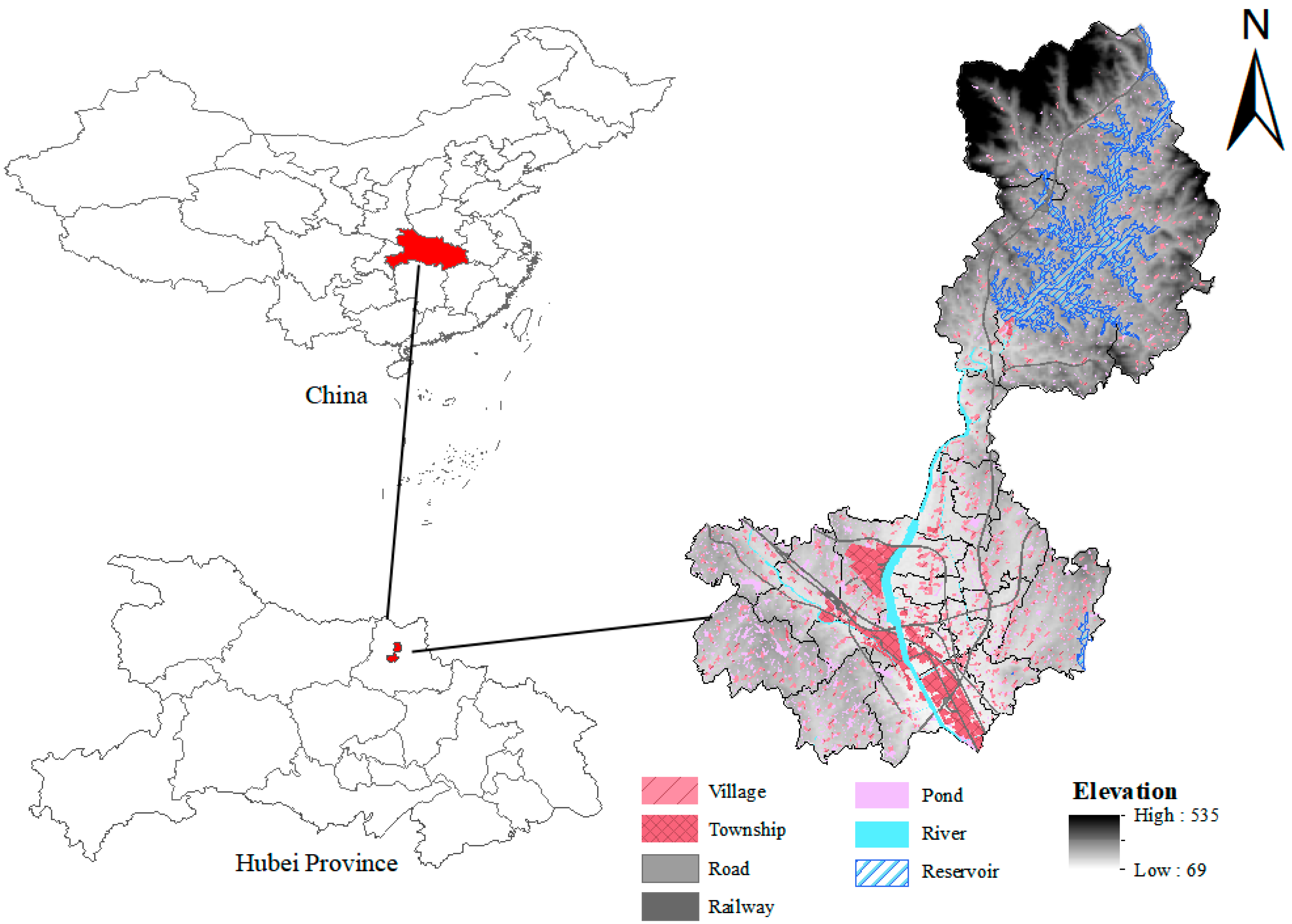
2. Study Area and Data Sources

Lishan Town is affiliated with Suizhou City, Hubei Province, and is the seat of the county government. It spans from 113°12′ to 113°29′ east in terms of longitude and 31°46′ to 32°06′ north in terms of latitude. The area of the township is 237.10 km². The area of cultivated land is 89.61 km², mainly in the form of paddy fields [39]. It has jurisdiction over 25 villages (including village committees) (Figure 1 and Figure 2). It is connected to Tongbai Mountain in the north, Dahong Mountain in the south, Xinyang in the east, Jingzhou and Fuyang in the west, and Handan, the Xining Railway and National Highway 316. It is an important transportation destination in northwest Hubei. There are many landforms in the territory, including complex terrain and typical regional characteristics of northwestern Hubei such as low hills in the north, alluvial plains in the south, and mountains with an altitude of 70–1140 m. There are many rivers in the town, such as the Lishui, Fengjiangkou and Dujia rivers. The subtropical monsoon climate of Lishan Town is characterized by good light and water conditions. The average annual precipitation is approximately 960 mm, the annual average temperature is 15.41 °C, and the annual frost-free period is approximately 220–240 days [40]. The farming culture has a long history.

The land use data of Lishan Town, Suizhou City, Hubei Province, in 2009 and 2015 was derived from the Suizhou Land Use Change Survey Database, which was provided by the Suizhou Land and Resources Bureau Information Center. In data processing, the analysis tools of ArcGIS 10.2 software (ESRI, 380 New York Street, Redlands, CA, USA) were used to extract the layers of cultivated land, villages, roads and water system elements in Lishan Town in 2009 and 2015, and then the spatial connection tool was used to associate the cultivated land elements with the administrative village vector diagrams. The digital elevation model (DEM) data (30 × 30 m) was downloaded from the Geospatial Data Cloud website (http://www.gscloud.cn/) for analysis of the elevation and slope of Lishan Town. These provide effective data support for the research in this paper.

3. Methods

3.1. Kernel Density Estimation (KDE)

The kernel density estimation method is a conventional statistical method using nonparametric density estimation, which can effectively detect and identify the hot spots and cold zone clusters in the study area [41]. Generally, the higher the kernel density value is, the higher the spatial distribution density of geographic elements. In contrast, the lower the kernel density value is, the smaller the spatial distribution density of geographic features. The specific principles of the KDE method are as follows: it takes each sample point $xi$ as the center and calculates the density contribution value of each grid center point of each sample within the specified radius ($h$) by the kernel function, and searches for the grid center point within the radius range. The closer the sample is, the larger the density value. In the kernel density estimation, the determination or selection of the search radius ($h$) has a great influence on the calculation result. As the $h$ increases, the point density change in space is smoother, but it masks the density structure; when $h$ decreases, the density change will be abrupt [42].

This article first uses the Feature to Point tool to convert the cultivated land data into point data, that is, extract the centroid of the polygon of cultivated land, and then use the Kernel Density tool to complete the kernel density estimation of the point data. After repeated trials, it was determined that an 800-m search radius be used to estimate the kernel density of the cultivated land spatial distribution, as this can achieve better results on the kernel density distribution map of the cultivated land in Lishan Town. The formula is as follows:

$$fn=\frac{1}{nh}{\displaystyle \sum }_{i=1}^{n}k\left(\frac{x-xi}{h}\right)$$

(1)

In Formula (1), $fn$ represents the kernel density value of the spatial distribution of cultivated land in the study area, $n$ represents the number of cultivated lands, $k$ represents the function of kernel density measurement, $xi-xj$ represents the distance between cultivated land $xi$ and cultivated land sample $xj$ in the study area, and $h$ represents the search radius.

3.2. Global Spatial Autocorrelation Analysis

The Global Moran’s I index can comprehensively detect the spatial self-phase size of spatial elements or their attribute values in a certain area and is generally used to study the spatial pattern of geographic elements and its evolution analysis [43]. Usually, under the confidence level of Zscore > 1.96 or Zscore < 1.96 (α = 0.05), the value of Zscore is between [–1,1]. If Zscore > 0, then there is a significant positive correlation of geographical features in space, indicating a spatial distribution feature of agglomeration; otherwise, Zscore < 0, indicating that the geographic feature has a significant negative correlation in space, and it has discrete spatial distribution features. This study uses the index to estimate the global spatial autocorrelation of the proportion of cultivated land in the administrative village [44], and the formula is as follows:

$$I=\frac{n{{\displaystyle \sum }}_{i=1}^n{{\displaystyle \sum }}_{j\ne i}^n\omega ij\left(xi-\overline{x}\right)\left(xj-\overline{x}\right)}{n{{\displaystyle \sum }}_{i=1}^n{{\displaystyle \sum }}_{i\ne j}^n\omega ij{\left(xi-\overline{x}\right)}^2}$$

(2)

$$Zscore=\frac{I-E\left(I\right)}{\sqrt{var\left(I\right)}}$$

(3)

In Formula (2), $n$ is the total number of administrative village spatial units, $xi$ and $xj$ are the observed values of the cultivated area ratio on the spatial regional units $i$ and $j$, $\overline{x}$ is the proportion of cultivated land in the study area, and ${\omega }_{ij}$ is the spatial weight matrix.

In Formula (3), $E\left(I\right)$ represents the expected value of Moran’s I and $VAR\left(I\right)$ represents the variance of Moran’s I.

3.3. Local Spatial Autocorrelation Analysis

Global space autocorrelation has certain limitations, and it cannot completely and accurately determine the specific location of spatial geographic feature aggregations and anomaly distributions in an entire region [45]. However, local spatial autocorrelation is a geostatistical method that can reflect the local correlation of spatial geographic feature location attributes, which can effectively show the correlation between the research area elements and the neighboring element attributes. The Moran scatter plot and the local indicators of spatial association (LISA) are used in this paper.

The Moran scatter plot is a statistical graph method that reflects the local autocorrelation of spatial position attributes. It is drawn using the data (X, W_X ), where the horizontal axis corresponds to the description variable X and the vertical axis corresponds to the spatial lag vector W_X. The four quadrants of the scatter plot correspond to the four local spatial association types: The first quadrant (H–H) represents that the high-valued region is surrounded by high-value neighbors, the second quadrant (L–H) represents that the low-value region is surrounded by high-value neighbors, the third quadrant (L–L) represents that the low-value region is surrounded by low-value neighbors, and the fourth quadrant (H–L) represents a high-valued area surrounded by low-value neighbors. Of these, the 1,3 quadrant and the 2,4 quadrants, respectively, indicate that there is a significant positive and negative spatial autocorrelation relationship between geographical elements. Since the Moran scatter plot does not reflect the level of significance of the spatial association type, the LISA analysis method needs to be introduced.

In general, the LISA can be used to measure the similarity (positive correlation) or difference (negative correlation) of the observation unit attribute value to the surrounding unit attribute value. At a given level of significance, if I > 0, indicating that there is a positive local spatial autocorrelation, similar values are agglomerated. However, if I < 0, there is a negative local spatial autocorrelation, and dissimilar values are agglomerated. Combining the LISA significance level with the Moran scatter map can form a LISA cluster map, which can clearly identify the “hot spots” and “cold spots” of local spatial agglomeration, revealing the degree of difference between agglomeration and isolation between spatial and adjacent features [46,47]. The formula is as follows:

$$I=\frac{\left(xi-\overline{x}\right){\displaystyle \sum _{j=1}^n{\omega }_{ij}\left(xj-\overline{x}\right)}}{{{\displaystyle S}}^2}$$

(4)

$${{\displaystyle S}}^2=\frac{1}{n}{\displaystyle \sum _{i=1}^n{\left(xi-\overline{x}\right)}^2}$$

(5)

The meanings of the relevant geographic element variables of Formulas (4) and (5) are the same as Formulas (2) and (3).

3.4. Spatial Weight Matrix

Selecting a suitable spatial weight matrix is an essential prerequisite for spatial autocorrelation analysis. In general, the spatial weight matrix can be divided into three weighting matrices based on the adjacency relationship, the distance, and the k-nearest point according to the spatial positional relationship. The method for determining the weight matrix based on the adjacency relationship may be divided into Rooks, Queens, Bishops, Kings, etc., according to the adjacency relationship of the spatial position. In this study, the administrative village is used as the spatial evaluation unit. The adjacency matrix is determined according to the above four adjacent relationships, and various adjacency relationships are analyzed to obtain a spatial adjacency frequency histogram. After repeated trials, the results based on the Rooks adjacency relationship are in line with the normal distribution characteristics of the cultivated land in the administrative village of Lishan Town. Therefore, this paper chooses the Rooks adjacency to determine the spatial weight to calculate the global Moran’s I and LISA.

3.5. Topographic Position Index

Topographical factors have an important influence on the spatial distribution of cultivated land elements. A single elevation or slope does not accurately reflect the degree of impact [48]. Therefore, this paper introduces the topographical position index (comprehensive calculation of elevation and slope) to characterize the spatial distribution characteristics of cultivated land. The formula is as follows:

$$T=log\left[\left(\frac{E}{\overline{E}}+1\right)\cdot \left(\frac{S}{\overline{S}}+1\right)\right]$$

(6)

In Formula (6), $T$ represents the topographic position index of any grid; $E$ represents the value of the elevation corresponding to any point in the study area, $\overline{E}$ represents the average of the elevation of the study area; $S$ represents the value of the slope corresponding to any point in the study area, and $\overline{S}$ represents the average of the slope of the study area.

3.6. Spatial Autoregressive Model

Previous research results show that a traditional ordinary least squares (OLS) regression model does not fully consider the spatial correlation between geospatial elements [49,50], and the spatial dependence of variables and their residual terms has an important impact on the accuracy of regression results [51,52]. When the spatial dependence between variables is critical to the model and leads to spatial correlation, that is, the neighboring value of the dependent variable has a direct impact on itself, this model is called the Spatial Lag Model (SLM). It explores whether there is a diffusion phenomenon (spill effect) in each region of each variable. When the spatial dependence is a result of the error, rather than the model itself, that is, the error terms of the model are spatially related, the model is called the Spatial Error Model (SEM) [53,54]. The SEM model explores whether there is a sequence correlation between the error terms.

In consideration of this, the SLM or SEM model can be used to more effectively reflect the autocorrelation of spatial regression. This paper takes the administrative village of Lishan Town as the research unit and selects the average value of the kernel density of cultivated land in each administrative village in 2009 and 2015 as the explanatory variable. Topographic position index (elevation, slope), village (administrative village, established town), road (railway, highway, rural road), and water system (river, lake and pond) all have different effects on the distribution of cultivated land. From the perspective of township standards, most of the cultivated land is distributed in the most suitable place for cultivation, and the place is mainly considered from the aspects of cultivation natural conditions and socio-economic conditions. From the perspective of natural conditions, small areas do not have large spatial heterogeneity in terms of climate and soil, but the microclimate formed by micro-geomorphology such as altitude and slope is a key factor affecting the development of cultivated land. That is to say, altitude and slope affect the distribution of cultivated land to a large extent, so it is necessary to analyze them as the influential factors. From the perspective of social economy, the accessibility of roads, the ease of irrigation, and the distance from villages are important indicators for measuring the suitability of cultivated land. Human beings are more inclined to open up cultivated land in the most convenient transportation, most convenient irrigation, and the nearest place to the village. In small areas, these factors cannot be optimal at the same time, so it is necessary to explore how these factors specifically affect the spatial distribution of cultivated land. On the basis of previous research [55,56,57], taking the administrative village of Lishan Town as the research unit, the average value of the kernel density of cultivated land in each administrative village is selected as the explanatory variable. We can also take the average value of the topographical position index of the elements of the cultivated land location of Lishan Town, the average value of the nearest distance from the cultivated land location elements to the village, the average distance of the nearest distance to the road, and the average distance of the nearest distance to the water system and use them as explanatory variables, to explore the impact of various factors on cultivated land from the township scale. The spatial autoregressive model is as follows:

$$y=\rho Wy+X\beta +\epsilon$$

(7)

$$y=\beta X+\epsilon ,\epsilon =\lambda W\epsilon +\mu$$

(8)

In Formulas (7) and (8), $y$ is the dependent variable, $X$ is a matrix comprising exogenous explanatory variables, $W$ is the spatial weights matrix of $n\times k$ ($n$ is the number of research units, $k$ is the number of independent variables); $\rho$, $\beta$, and $\lambda$ are the corresponding coefficients ($\rho$ and $\lambda$ reflect the strength of spatial dependence.); and ε and $\mu$ are the random error term vectors.

4. Results and Analysis

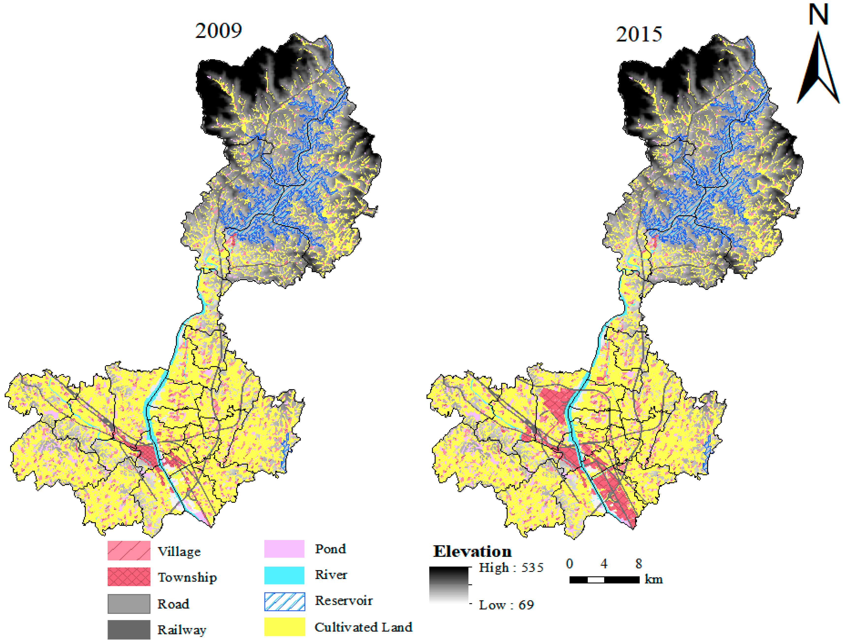
4.1. Distribution and Variation Characteristics of Regional Cultivated Land

On the whole, the total amount of cultivated land in Lishan Town is decreasing, it is mainly distributed in the north and southwest, and there are fewer administrative villages with increased amounts of cultivated land. From 2009 to 2015, the cultivated area of Lishan Town dropped from 9211.97 hm² to 8725.28 hm². At this time scale, the regional differences in the spatial change of cultivated lands in Lishan Town are obvious. The specific performances are as follows: from 2009 to 2015, Beigang Village in the north of Lishan Town and Xingju Village in the south had large reductions in the area of cultivated land. The cultivated land area was reduced by 3.68 hm², accounting for 75.69% of the total area of cultivated land reduction. Second, the administrative villages with large reductions in the area of cultivated land in Lishan Town were the Qinlao Village in the north, Xingqi Village in the central part and Shuangxing Village in the southwest. The reduced area of cultivated land was 65.80 hm², accounting for 13.52% of the total area of cultivated land reduction; the reduction of cultivated land in the village was relatively small, and the reduction area was less than 10.00 hm². The only administrative villages with increased cultivated land are the Dongxin Village in the east and the Haichaosi Village in the northeast, but the increased area of cultivated land was only approximately 2.00 hm². During the research period, due to the rapid development of urbanization construction in Lishan Town, the area of cultivated land converted into construction land was 4.92 hm².

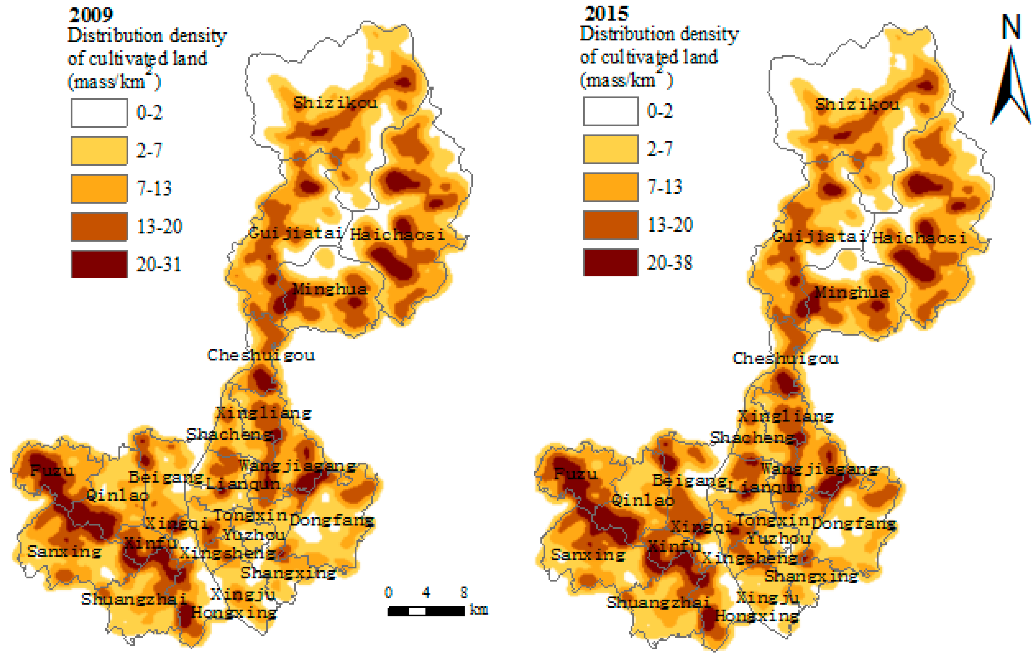
4.2. Kernel Density Analysis of Cultivated Land

Using the kernel density analysis tool in ArcGIS 10.2, we can calculate the kernel density values of cultivated land in Lishan Town in 2009 and 2015 and use the natural spacing method to divide the kernel density values of the spatial distribution of cultivated land in 2009 into five grades. The ranks are 0~2 blocks/km², 2~7 blocks/km², 7~13 blocks/km², 13~20 blocks/km² and 20~31 blocks/km². Based on the classification of 2009, 2 blocks/km², 7 blocks/km², 13 blocks/km², 20 blocks/km² and 38 blocks/km² can be used as the boundary values of the kernel density classification for cultivated land spatial distribution in 2015 (Figure 3). This shows that the maximum values of the kernel density distribution of cultivated land spatial distribution in Lishan Town in 2009 and 2015 were 31/km² and 38/km², respectively, indicating that there was a small increase in the distribution of cultivated land in some administrative villages, and the degree of cultivated land agglomeration was strengthened in Lishan Town between 2009 and 2015. From Figure 4, the kernel density distribution of cultivated land has the following characteristics: (1) In 2009 and 2015, the high-density areas of cultivated land distribution in Lishan Town were concentrated in the flat areas of the southwest and northeast, including the Fuyu Village, Qinlao Village and Haichaosi Village, and a small part of Wangjiagang Village. The median areas of kernel density were concentrated in the southeast plain area and the northern mountainous area, including the eastern part of Tongxin Village, the southern part of Xingsheng Village and the northern part of Guijiatai village. In addition, the lower areas of kernel density were concentrated in the northern part of the Shizikou Village, a part of the Haichaosi village and the eastern part of the Dongfang Village. (2) From 2009 to 2015, the areas of cultivated land kernel density with 20 blocks/km² and above were mainly distributed in Fuzu Village, Qinlao Village, Xingfu Village, Wangjiagang Village and Haichaosi Village, with other administrative villages exhibiting less; there was a wide distribution for land kernel densities between 13~20 blocks/km², including most of the areas of Xingfu Village, Beigang Village, Hongxing Village, Xingliang Village, Mingtai Village and Shikou Village, and a part of Fuzu Village, Qinli Village and Haichaosi Village. In particular, the area centered on Fuzu Village, Qinlao Village and Haichaosi Village has a tendency to spread to higher-value areas, while the distribution areas of cultivated land kernel density values of between 7 and 13 blocks/km² are mainly concentrated in Shuangzhai Village, Shuangxing Village, Xingsheng Village, and Dengta Village. However, on the whole, the regional change in the kernel density of cultivated land over two years was small, and other areas with low kernel density values were mainly concentrated in a few administrative villages in the northern mountainous areas. The distribution of cultivated land in this area is partially expanded or sporadic, but has not changed much. According to the analysis of the above changes, it can be seen that the distribution of cultivated land in Lishan Town is relatively concentrated and is mainly distributed in the southwest and eastern flat areas. The density of cultivated land in the northern mountainous areas of Lishan Town is significantly lower than that in the southwest and eastern plains, indicating that topographic factors have a greater impact on the spatial distribution of cultivated land.

4.3. Analysis of Autocorrelation in Cultivated Land

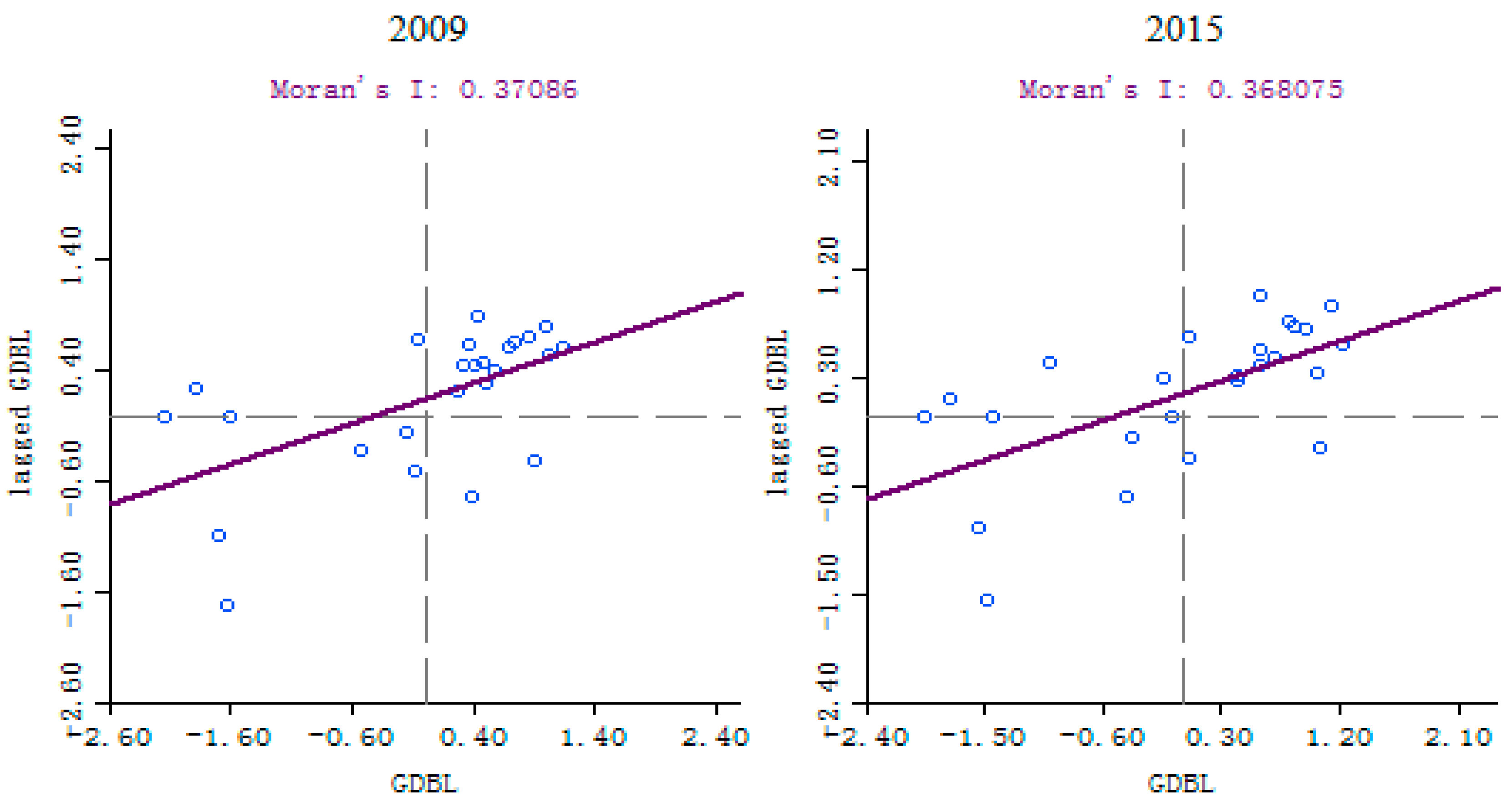
4.3.1. Global Spatial Autocorrelation

We used Geoda (Center for Spatial Data Science Computation Institute, Chicago, IL, USA) to calculate the global spatial autocorrelation index of the ratios of cultivated land areas in each administrative village of Lishan Town in 2009 and 2015. The specific results are shown in

Table 1. Global Moran’s I index and test of the proportion of cultivated land area in administrative village of Lishan Town in 2009 and 2015.

Year	Moran’s I	Zscore	$\mathbf{Threshold}\mathbf{Value}(\mathit{\alpha }=0.05)$
2009	0.5251	6.343	1.96
2015	0.3970	4.820	1.96

.

From Table 1, the global spatial autocorrelation index values of Moran’s I of the proportion of cultivated land area in the administrative villages of Lishan Town in 2009 and 2015 were 0.5251 and 0.3970, respectively, which were far greater than 0. The normalized value Zscores are 6.343 and 4.820, respectively, which are also much larger than the significant horizontal threshold of 1.96, both of which pass the significance level test. This shows that there is a significant spatial autocorrelation between the proportion of cultivated land in the administrative villages of Lishan Town in 2009 and 2015, and there is a strong agglomeration phenomenon, which is reflected in the vicinity of the administrative villages adjacent to a higher proportion of cultivated land, and the proportion of cultivated land is also correspondingly higher. In contrast, the proportion of cultivated land in the vicinity of the administrative villages near the lower cultivated area is also low. Judging from the trend of the global autocorrelation index value Moran’s I, the autocorrelation of cultivated land in each administrative village of Lishan Town has a weakening trend from 2009 to 2015.

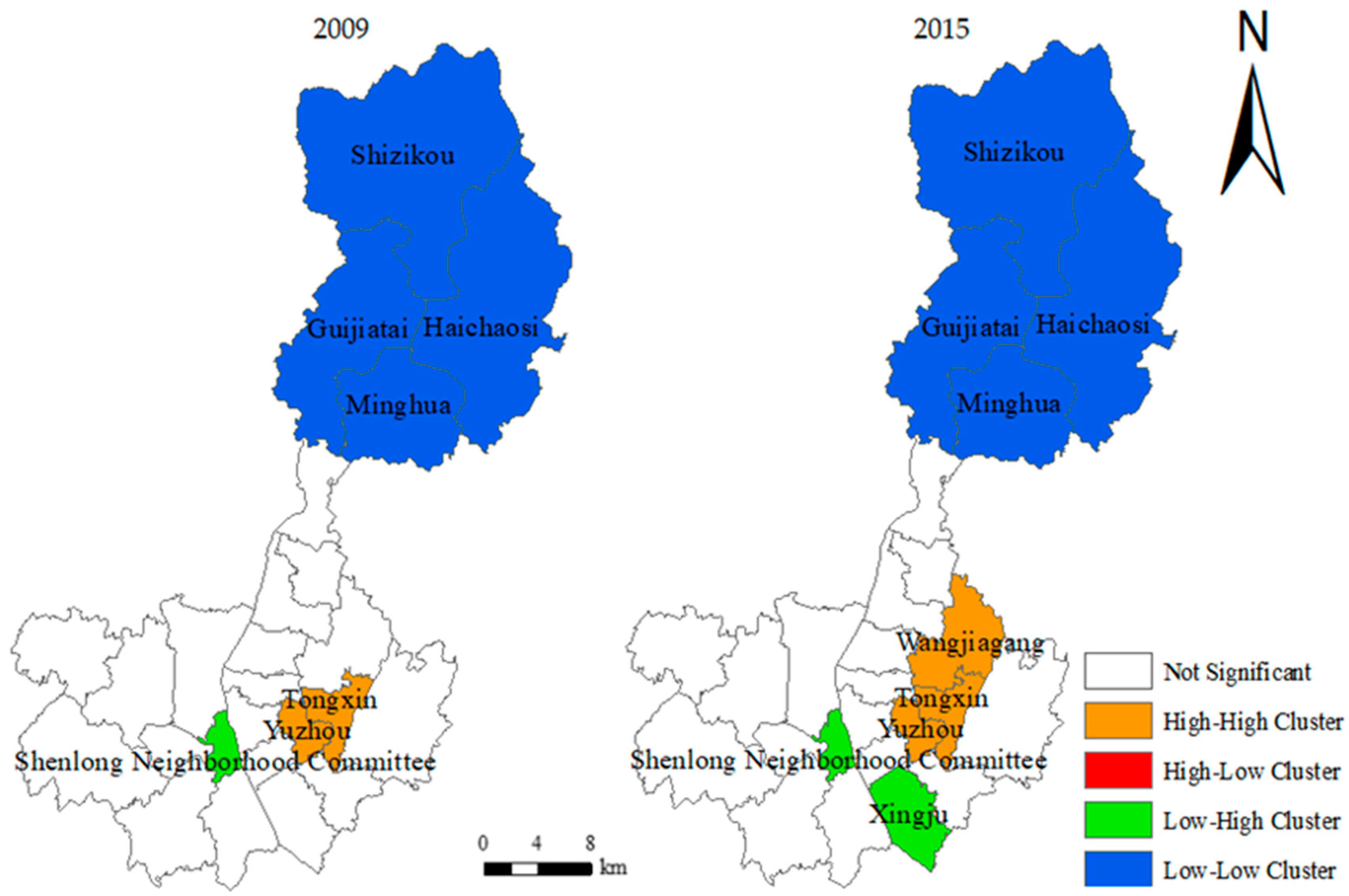
4.3.2. Local Spatial Autocorrelation

From the perspective of global spatial autocorrelation analysis, the cultivated land of Lishan Town has a strong agglomeration distribution in space. However, considering the spatial distribution of the kernel density values of cultivated land determined above, the distribution of cultivated land in each administrative village still exhibits obvious differences. By using the local spatial autocorrelation statistics, it is possible to more accurately analyze the internal differences in the spatial autocorrelation levels of the cultivated land area of each administrative village in Lishan Town. The Geoda software was used to map the spatial autocorrelation Moran’s I scatter plot corresponding to the proportion of cultivated land in each administrative village of Lishan Town in 2009 and 2015 (Figure 4).

Figure 4 shows the spatial distribution characteristics of cultivated land in each administrative village of Lishan Town. Specific features are as follows: (1) On the whole, the spatial autocorrelation Moran’s I scatter plots of the proportions of the cultivated land area of the administrative villages in the two years are mainly “H–H” and “L–L” types. Of these, there are 19 and 17 administrative villages within the two types of accumulation in 2009 and 2015, respectively, accounting for 76% and 68% of the total administrative villages; there are more administrative villages belonging to the “H–H” type, and there is a significant aggregation distribution in the cultivated land space of this type. However, the number of administrative villages belonging to the “L–H” and “H–L” types is small, and the two types of cultivated land have obviously discrete distribution characteristics. (2) Over this time, the number of administrative villages belonging to the type of “H–H” and “L–L” types fell from 19 in 2009 to 17 in 2015, and the spatial heterogeneity of the localities was weakened. However, the number of corresponding “L–H” and “H–L” types of administrative villages increased slightly, indicating that the spatial diffusion scope of cultivated land in the administrative villages of the respective types had been decreased, and the spatial heterogeneity of the areas had slightly increased. On the whole, the cultivated land of the administrative villages with higher or lower proportions of cultivated land in Lishan Town was characterized by agglomeration and contraction distributions from 2009 to 2015.

To more intuitively express the degrees of difference in the proportions of cultivated land area of each administrative village and its changing trend in Lishan Town, we mapped the LISA agglomeration of cultivated land in the administrative village of Lishan Town at a significance level of α = 0.05 (Figure 5). As seen from the figure, the LISA agglomeration map has the following characteristics: (1) “H–H” type zone. This type of area belongs to administrative village space units with a high proportion of cultivated land area and a correspondingly high proportion of cultivated land area in the surrounding area. The specific characteristics are that the ratio of cultivated land area in this type of area is relatively high, and the spatial difference between adjacent units is relatively small. The local spatial heterogeneity is weak, and is mainly distributed in the central part of Lishan Town. On the whole, regions of this type have expanded eastward from 2009 to 2015. In 2009, they were mainly concentrated in Tongxin Village and the Yuzhou Village in the middle of Lishan Town; in 2015, this type of district included Tongxin Village and Yuzhou Village and included Wangjiagang Village in the eastern part of Lishan Town. (2) “L–L” type zone. This type of area belongs to the administrative village spatial units with a low proportion of cultivated land area and a low proportion of cultivated land in the surrounding neighboring units. This shows that the ratio of cultivated land area between the spatial unit and its surrounding area is low, the local spatial difference is small, and it still shows a state of agglomeration distribution in space. The area is mainly dominated by mountainous terrain, with large slopes, large distributions of forests and few cultivated lands, including Shizikou Village, Haichaosi Village, Guijiatai Village and Minghua Village in the northern mountainous areas of Lishan Town. From 2009 to 2015, the area of cultivated land in this type of area was generally reduced, and the reduction of cultivated land area in the middle of Minghua Village was particularly obvious, indicating that due to ecological construction and the policy of returning farmland to forests in the northern mountainous areas, the cultivated land has been partially reduced. (3) “H–L” type zone. From 2009 to 2015, no administrative villages of Lishan Town were distributed in this area, so no analyses were made. (4) “L–H” type zone. This type of area belongs to administrative village space units with a low proportion of cultivated land and a relatively high proportion of cultivated land adjacent to the unit, and the spatial relationship shows a negative correlation and a strong spatial heterogeneity. The specific representation is that the proportion of cultivated land is relatively low, and the proportion of cultivated land adjacent to it is obviously high, forming a local spatial heterogeneity “hot spot”. It can be seen from Figure 6 that the number of administrative village space units in this type of area is very small, and the “hot spot” area in 2009 is the Shenlong Neighborhood Committee, while the “hot spot” area in 2015 is the Shenlong Neighborhood Committee and Xingju Village.

4.4. Spatial Autocorrelation Regression Analysis of Influencing Factors of Cultivated Land

4.4.1. Selection of the Model

Since it is difficult to judge whether spatial dependence is derived from the variable itself or the error term of the model in empirical research, it is necessary to decide which spatial autoregressive model is more in line with objective reality according to the specific discriminant criterion [58]. Anselin proposed the following criterion [59,60]: If the Lagrange Multiplier (LM) and its robust (Robust Lagrange Multiplier) form of LM–LAG (Lagrange Multiplier–lag) are found in the spatial dependence test, LM–LAG compared to LM–ERR (Lagrange Multiplier–error) is statistically more significant, and Robust LM–LAG is significant and Robust LM–ERR is not significant, then it can be concluded that the appropriate model is a spatial lag model [61]. Conversely, if LM–ERR is more statistically significant than LM–LAG, and Robust LM–ERR is significant and Robust LM–LAG is not significant, then it can be concluded that the spatial error model is a more appropriate model. We used the spatial dependence analysis of the Geoda software platform (

Table 2. Spatial dependency test.

Test	2009			2015
	MI/DF	Value	p	MI/DF	Value	p
Langrange Multiplier(lag)	1	119.417	0.000	1	25.510	0.000
Robust LM(lag)	1	27.134	0.000	1	0.973	0.410
Langange Multiplier(error)	1	175.289	0.000	1	58.156	0.000
Robust LM(error)	1	67.158	0.000	1	32.754	0.000

) and determined the specific regression model based on the selection criteria proposed by Anselin [62].

As can be seen from Table 2, the statistical tests of LM-LAG, Robust LM–LAG, LM–ERR and Robust LM–ERR were significant (p = 0) in 2009, and it seems impossible to judge whether the spatial lag model or the spatial error model is more suitable. Although the statistical tests of LM–LAG and LM-ERR are significant (p = 0) in 2015, and Robust LM-ERR is significant (p = 0), Robust LM-LAG is not significant (p = 0.41), so the spatial error model (SEM) is more suitable for analyzing the autocorrelation regression of the driving factors of the spatial distribution of cultivated land in Lishan Town.

4.4.2. Analysis of Regression Results

To reduce the influence of heteroscedasticity on the accuracy of regression results, this paper performs a natural logarithmic transformation of all variables, which makes the results of the analysis easy to compare (similar to standardization) [57]. The SEM regression analysis was performed by the spatial measurement tool in MATLAB (The Math Works Inc, Natick, Massachusetts, USA) software, and the results are shown in

Table 3. Regression results of spatial error model (SEM).

Item	2009				2015
Variables	Coefficient	Standard Deviation	Z-Value	p	Coefficient	Standard Deviation	Z-Value	p
Constant	−20.095	0.904	−22.223	0.000	−19.134	0.789	−24.249	0.000
To the nearest village	0.236	0.083	11.096	0.000	0.196	0.081	2.424	0.000
To the nearest road	0.632	0.057	11.096	0.000	0.630	0.056	11.288	0.000
To the nearest water systems	0.481	0.099	4.855	0.000	0.290	0.080	3.610	0.015
Topographic position index	−0.817	0.206	−3.957	0.005	−0.672	0.202	−3.332	0.001
LAMBDA	0.796	0.069	11.485	0.000	0.828	0.063	13.076	0.000

.

Based on the principles of geography and geostatistics, the SEM regression results in Table 3 and Figure 6 can further reveal the regression mechanism and spatial autocorrelation between the spatial distribution of cultivated land and the influence degree of its driving factors [63]. The specific conclusions are as follows:

In 2009 and 2015, the spatial distributions of cultivated land in Lishan Town, as well as the topographical position index and the closest distance from the cultivated land to the village (administrative village, established town), the road (railway, highway, rural road) and the water systems (river, lake and pond), have a significant impact on the spatial distribution of cultivated land, and the four influential factors pass the significance test (all the p values are less than 0.05). Judging from the degree of influence of the spatial distribution drivers of cultivated land, the distribution of cultivated land is basically consistent with its natural geographical conditions. Specifically, the regression coefficient of the topographic index is negative, and the regression coefficients of the other three influencing factors are positive. In other words, the higher the value of the topographical position index of Lishan Town, the less cultivated the land is, but in areas where cultivated land is closer to a village, road or water system, the land is more cultivated.

The regression coefficient of the impact factor is an important indicator reflecting the degree of its impact. In 2009 and 2015, the absolute values of the regression factors of the influencing factors of cultivated land space in Lishan Town are in ascending order: topographic position index (0.817, 0.672), the nearest distance to the road (0.632, 0.630), the nearest distance to the water systems (0.481, 0.290), and the nearest distance to the township (0.236, 0.196). That is to say, in 2009 and 2015, the coefficient of the topographic position index of Lishan Town increased by 1%, and the spatial density of cultivated land decreased by 0.82% and 0.67%, respectively. In addition, the coefficient of the distance from villages, roads and water systems increased by 1%, the spatial density of cultivated land will increase by 0.24%, 0.20%, 0.63%, and 0.63%, 0.48%, and 0.29%, respectively. From this outcome, it can be judged that the topographical factors have the highest impact on the spatial distribution of cultivated land, which is mainly due to the development and protection of cultivated land that is not suitable for areas with higher terrain and steep slopes. Second, the distribution is greatly affected by the distance from roads and water systems, the less distance there is to rural roads, the more conducive it is to the mechanization of large-scale agricultural machinery, which therefore promotes the level of agricultural production. The areas where the water system in Lishan Town flows are mainly plains, most of which are paddy fields, characterized by flat terrain, gentle slopes and high soil fertility. In addition, water systems (river, lake and pond) can provide important irrigation water sources for agricultural production; therefore, the shorter the distance to a water system, the more cultivated land there is. The close distance between the cultivated land and the village is another important factor that affects the distribution of cultivated land. However, from the perspective of field research, due to the development and improvement of modern agricultural technology, and the strengthening of national efforts to promote land remediation planning, the influence of village distance on the distribution of cultivated land is not as strong as in traditional thinking.

According to the degree of influence of different years, and comparing 2015 with 2009, the regression coefficients of each influencing factor were reduced by varying degrees. It is further indicated that with the development of society and the advancement of agricultural technology, the level of modern agricultural development in China is continuing to increase along with the influence of the topographic position index, while the distances to villages, roads and water systems on the spatial distribution of cultivated land are gradually reduced. In general, the results of the degree of influence on the spatial distribution drivers of cultivated land are consistent with the reality of Lishan Town.

5. Conclusions and Discussion

Based on geographic information technology, this study is based on the plow map layer of Lishan Town in 2009 and 2015, and using the kernel density analysis, cultivated land concentration indexes, spatial autocorrelation analysis, SEM and other methods to analyze the spatial distribution characteristics and influencing factors of cultivated land, the following conclusions can be drawn:

(1) From the distribution of high and low kernel density values, the kernel density of cultivated land in Lishan Town in 2009 and 2015 showed a strong agglomeration distribution in space. The high-value areas of kernel density are mainly distributed in the southwestern part and the northeastern part of the country, concentrated in the Fuzu Village, most areas of Qinlao Village and parts of Haichaosi Village and Wangjiagang Village. The low-value areas are mainly concentrated in the northern part of the Shizikou Village, Haichaosi Village, the southeastern Dongfang Village, Shuangxing Village and Xingju Village. On the whole, the spatial distribution density of cultivated land in the northern mountainous areas of Lishan Town from 2009 to 2015 is significantly lower than that in the southwest plain area, indicating that the spatial distribution of cultivated land in the region is greatly affected by topographic factors.

(2) Judging from the spatial autocorrelation of cultivated land, the global spatial autocorrelation Moran’s I of the proportion of cultivated land area in the administrative village of Lishan Town in 2009 and 2015 was 0.5251 and 0.3970, and the spatial autocorrelation of cultivated land distribution is significant. The high- or low-value areas of cultivated land area in administrative villages have obvious agglomeration distribution characteristics in space, but the spatial heterogeneity of cultivated land in administrative villages is stronger. The agglomeration area with the highest proportion of cultivated land area is located in the southern part of Cheshuigou Village, mainly concentrated in Tongxin Village and Yuzhou Village; the agglomeration area with the lowest proportion of cultivated land is distributed in the mountainous area in the north of Cheshuigou Village, and the “hot spot” area in 2009 was the Shenlong Neighborhood Committee, while the “hot spot” area in 2015 was the Shenlong Neighborhood Committee and Xingju Village.

(3) Based on the previous research results [64,65,66], a spatial autoregressive model is introduced to quantitatively study the influence mechanisms of natural geographical environment on the spatial distribution of cultivated land. The results show that the four factors have different effects on the spatial distribution of cultivated land in Lishan Town, and the absolute values of the regression coefficients of the influencing factors of the cultivated land space over two years are, in ascending order: topographic position index, the nearest distance to the road, the nearest distance to the water system, the nearest distance to the township. Comparing 2015 with 2009, the regression coefficients of each influencing factor were reduced to varying degrees. It is further indicated that with the development of society and the advancement of agricultural technology, the level of modern agricultural development in China continues to increase, and the influence of topographic indices, the nearest distance to villages, and roads and water systems on the spatial distribution of cultivated land are gradually reduced, and this result is consistent with the actual situation in the study area.

Cultivated land resources are basic resources for human survival and socially sustainable development, and the study of spatial distribution and its influential factors is a long-term dynamic process. Based on the plow map layer of Lishan Town in 2009 and 2015, the author used a GIS spatial analysis method, a spatial autocorrelation model and the SEM to analyze the spatial distribution characteristics of cultivated land and the degree of its influential factors from the township scale. In the existing research [67,68,69], in order to more reasonably promote the sustainable use of cultivated land, many scholars have explored the influence factors of the spatial distribution of cultivated land, but most of the research has focused on larger scales. In the paper, the authors take a typical area as a case to improve and enrich the research on the spatial-temporal characteristics of cultivated land and the influence of different natural factors from the micro scale. However, due to the obvious differences in nature and socio-economics in different regions, it is also affected by regional government policies, planning and data incompleteness. The results of this study may deviate from the actual research area. The research on the spatial and temporal distribution characteristics of cultivated land and the degree of its influential factors in this article is far from enough, and cannot represent the current status of cultivated land in the world. However, the spatial and temporal differentiation characteristics of cultivated land in typical townships in China and the changes in the degree of influencing factors are an important microcosm of the change of cultivated land in the world. In future research, we must further strengthen the exploration of the influence of social economy, government policies and soil quality on the spatial distribution of cultivated land to provide better guidance for the optimal layout and sustainable use of cultivated land resources.

References

1. Tanrivermis, H. Agricultural land use change and sustainable use of land resources in the Mediterranean region of Turkey. J. Arid Environ. 2003, 54, 553–564. [Google Scholar] [CrossRef]
2. Song, W.; Pijanowski, B.C. The effects of China’s cultivated land balance program on potential land productivity at a national scale. Appl. Geogr. 2014, 46, 158–170. [Google Scholar] [CrossRef]
3. Zhao, W.W. Arable land change dynamics and their driving forces for the major countries of the world. Acta Ecol. Sin. 2012, 32, 6452–6462. [Google Scholar] [CrossRef] [Green Version]
4. The Statistical Database of the Food and Agriculture Organization (FAO). Available online: http://www.fao.org (accessed on 15 June 2019).
5. EL-kawy, O.R.A.; Ismail, H.A.; Yehia, H.M.; Allam, M.B. Temporal detection and prediction of agricultural land consumption by urbanization using remote sensing. Egypt. J. Remote Sens. Space Sci. 2019. [Google Scholar] [CrossRef]
6. Radwan, T.M.; Blackburn, G.A.; Whyatt, J.D.; Atkinson, P.M. Dramatic Loss of Agricultural Land Due to Urban Expansion Threatens Food Security in the Nile Delta, Egypt. Remote Sens. 2019, 11, 332. [Google Scholar] [CrossRef]
7. Szewrański, S.; Kazak, J.; Żmuda, R.; Wawer, R. Indicator-based assessment for soil resource management in the Wrocław Larger Urban Zone of Poland. Pol. J. Environ. Stud. 2017, 26, 2239–2248. [Google Scholar] [CrossRef]
8. Deng, X.Z.; Huang, J.K.; Scott, R.; Zhang, J.P.; Li, Z.H. Impact of urbanization on cultivated land changes in China. Land Use Policy 2015, 45, 1–7. [Google Scholar] [CrossRef]
9. The Ministry of Natural Resources of the People’s Republic of China. Available online: http://www.mnr.gov.cn/dt/ywbb/201810/t20181030_2290463.html (accessed on 18 May 2018).
10. Xie, Y.C.; Mei, Y.; Guang, J.T.; Xue, R.X. Socio-economic driving forces of arable land conversion: A case study of Wuxian City, China. Glob. Environ. Chang. 2005, 15, 238–252. [Google Scholar] [CrossRef]
11. Tan, Y.T.; Xu, H.; Zhang, X.L. Sustainable urbanization in China: A comprehensive literature review. Cities 2016, 55, 82–93. [Google Scholar] [CrossRef]
12. Zu, J.; Hao, J.M.; Chen, L.; Zhang, Y.B.; Wang, J.; Kang, L.T.; Guo, S.H. Analysis on trinity connotation and approach to protect quantity, quality and ecology of cultivated land. J. China Agric. Univ. 2018, 23, 84–95. [Google Scholar]
13. The Milnistry of Nature Resources of the People’s Repulic of China. Available online: http://f.mlr.gov.cn/201712/t20171214_1702106.html (accessed on 11 December 2018).
14. Liu, T.; Liu, H.; Qi, Y.J. Construction land expansion and cultivated land protection in urbanizing China: Insights from national land surveys, 1996–2006. Habitat Int. 2015, 46, 13–22. [Google Scholar] [CrossRef]
15. Xie, H.L.; Wang, W.; Zhang, X.M. Evolutionary game and simulation of management strategies of fallow cultivated land: A case study in Hunan province, China. Land Use Policy 2018, 71, 86–97. [Google Scholar] [CrossRef]
16. Liu, X.W.; Zhao, C.L.; Song, W. Review of the evolution of cultivated land protection policies in the period following China’s reform and liberalization. Land Use Policy 2017, 67, 660–669. [Google Scholar] [CrossRef]
17. Liu, Y.S.; Wang, J.Y.; Long, H.L. Analysis of arable land loss and its impact on rural sustainability in Southern Jiangsu Province of China. J. Environ. Manag. 2010, 91, 646–653. [Google Scholar] [CrossRef] [PubMed]
18. Rounsevell, M.D.A.; Annetts, J.E.; Audsley, E.; Mayr, T.; Reginster, I. Modelling the spatial distribution of agricultural land use at the regional scale. Agric. Ecosyst. Environ. 2003, 95, 465–479. [Google Scholar] [CrossRef]
19. Chen, J.F.; Wei, S.Q.; Chang, K.T.; Tsai, B.W. A comparative case study of cultivated land changes in Fujian and Taiwan. Land Use Policy 2007, 24, 386–395. [Google Scholar] [CrossRef]
20. Huang, B.Q.; Huang, J.L.; Pontius, R.G., Jr.; Tu, Z.S. Comparison of Intensity Analysis and the land use dynamic degrees to measure land changes outside versus inside the coastal zone of Longhai, China. Ecol. Indic. 2018, 89, 336–347. [Google Scholar] [CrossRef]
21. Li, X.; Yeh, A.G.O. Modelling sustainable urban development by the integration of constrained cellular automata and GIS. Int. J. Geogr. Inf. Sci. 2000, 14, 131–152. [Google Scholar] [CrossRef]
22. Zhong, T.Y.; Huang, X.J.; Zhang, X.Y.; Wang, K. Temporal and spatial variability of agricultural land loss in relation to policy and accessibility in a low hilly region of southeast China. Land Use Policy 2011, 28, 762–769. [Google Scholar] [CrossRef]
23. Li, H.; Wu, Y.Z.; Huang, X.J.; Sloan, M.; Skitmore, M. Spatial-temporal evolution and classification of marginalization of cultivated land in the process of urbanization. Habitat Int. 2017, 61, 1–8. [Google Scholar] [CrossRef] [Green Version]
24. Xie, H.L.; Yao, G.R.; Liu, G.Y. Spatial evaluation of the ecological importance based on GIS for environmental management: A case study in Xingguo county of China. Ecol. Indic. 2015, 51, 3–12. [Google Scholar] [CrossRef]
25. Hua, Y.; Yan, M.; Li, M.D. Land ecological security assessment for Bai autonomous prefecture of Dali based using PSR model—With data in 2009 as case. Energy Procedia 2011, 5, 2172–2177. [Google Scholar] [CrossRef]
26. Liang, W.; Yang, Y.T.; Fan, D.M.; Guan, H.D.; Zhang, T.; Long, D.; Zhou, Y.; Bai, D. Analysis of spatial and temporal patterns of net primary production and their climate controls in China from 1982 to 2010. Agric. For. Meteorol. 2015, 204, 22–36. [Google Scholar] [CrossRef]
27. Long, H.L.; Liu, Y.S.; Wu, X.Q.; Dong, G.H. Spatio-temporal dynamic patterns of farmland and rural settlements in Su–Xi–Chang region: Implications for building a new countryside in coastal China. Land Use Policy 2009, 26, 322–333. [Google Scholar] [CrossRef]
28. Liu, J.Y.; Zhang, Z.X.; Xu, X.L.; Kuang, W.H.; Zhou, W.C.; Zhang, S.W.; Li, R.D.; Yan, C.Z.; Yu, D.S.; Wu, S.X.; et al. Spatial patterns and driving forces of land use change in China during the early 21st century. J. Geogr. Sci. 2010, 20, 483–494. [Google Scholar] [CrossRef]
29. Han, H.R.; Yang, C.F.; Song, J.P. Scenario simulation and the prediction of land use and land cover change in Beijing, China. Sustainability 2015, 7, 4260–4279. [Google Scholar] [CrossRef]
30. Yu, J.; Ning, J.; Dong, F.C.; Du, G.M.; Lou, G.; Zhao, Z. Distribution and evolutionary characteristics of cultivated lands in the north-east of Sanjiang Plain from 1950 to 2013. J. Arid Land Resour. Environ. 2017, 31, 79–86. [Google Scholar]
31. Xie, B.G.; Zeng, X.M.; Li, X.Q.; Deng, C.X.; Zhu, D.G. Research spatial layout optimization of rural residential land in land use planning at township—A case of Liaotian town in Hengnan county. Econ. Geogr. 2010, 10, 1700–1706. [Google Scholar]
32. Wang, H.; Long, H.L.; Li, X.B.; Yu, F. Evaluation of changes in ecological security in China’s Qinghai Lake Basin from 2000 to 2013 and the relationship to land use and climate change. Environ. Earth Sci. 2014, 72, 341–354. [Google Scholar] [CrossRef]
33. Zhang, W.T.; Huang, B. Land use optimization for a rapidly urbanizing city with regard to local climate change: Shenzhen as a case study. J. Urban Plan. Dev. 2014, 141, 05014007. [Google Scholar] [CrossRef]
34. Liu, J.Y.; Liu, M.L.; Tian, H.Q.; Zhuang, D.F.; Zhang, Z.X.; Zhang, W.; Tang, X.M.; Deng, X.Z. Spatial and temporal patterns of China’s cropland during 1990–2000: An analysis based on Landsat TM data. Remote Sens. Environ. 2005, 98, 442–456. [Google Scholar] [CrossRef]
35. Zheng, Y.M.; Chen, T.B.; He, J.Z. Multivariate geostatistical analysis of heavy metals in topsoils from Beijing, China. J. Soils Sediment 2008, 8, 51–58. [Google Scholar] [CrossRef]
36. Sun, B.; Zhou, S.L.; Zhao, Q.G. Evaluation of spatial and temporal changes of soil quality based on geostatistical analysis in the hill region of subtropical China. Geoderma 2003, 115, 85–99. [Google Scholar] [CrossRef]
37. Li, X.; Yeh, A.G.O. Analyzing spatial restructuring of land use patterns in a fast growing region using remote sensing and GIS. Landsc. Urban Plan. 2004, 69, 335–354. [Google Scholar] [CrossRef]
38. Gao, J.; Liu, Y.S.; Chen, Y.F. Land cover changes during agrarian restructuring in Northeast China. Appl. Geogr. 2006, 26, 312–322. [Google Scholar] [CrossRef]
39. The Bureau of Land Resource Suizhou. Available online: http://www.szgtzy.gov.cn/ (accessed on 2 August 2018).
40. The Bureau of Land Resource Suixian. Available online: http://www.zgsuixian.gov.cn/sxgt/ (accessed on 25 June 2018).
41. Rinner, C.; Hussain, M. Toronto’s urban heat island—Exploring the relationship between land use and surface temperature. Remote Sens. 2011, 3, 1251–1265. [Google Scholar] [CrossRef]
42. Lanorte, A.; Danese, M.; Lasaponara, R.; Murgante, B. Multiscale mapping of burn area and severity using multisensor satellite data and spatial autocorrelation analysis. Int. J. Appl. Earth Obs. Int. 2013, 20, 42–51. [Google Scholar] [CrossRef]
43. Griffith, D.A. Visualizing analytical spatial autocorrelation components latent in spatial interaction data: An eigenvector spatial filter approach. Comput. Environ. Urban 2011, 35, 140–149. [Google Scholar] [CrossRef]
44. Diniz-Filho, J.A.F.; Siqueira, T.; Padial, A.A.; Rangel, T.F.; Landeiro, V.L.; Bini, L.M. Spatial autocorrelation analysis allows disentangling the balance between neutral and niche processes in metacommunities. Oikos 2012, 121, 201–210. [Google Scholar] [CrossRef]
45. Oliveira, D.G.; Diniz-Filho, J.A.F. Spatial patterns of terrestrial vertebrate richness in Brazilian semiarid, Northeastern Brazil: Selecting hypotheses and revealing constraints. J. Arid Environ. 2010, 74, 1418–1426. [Google Scholar] [CrossRef]
46. Kawaguchi, D.; Yukutake, N. Estimating the residential land damage of the Fukushima kernel accident. J. Urban Econ. 2017, 99, 148–160. [Google Scholar] [CrossRef]
47. Fleming, C.H.; Calabrese, J.M. A new kernel density estimator for accurate home-range and species-range area estimation. Methods Ecol. Evol. 2017, 8, 571–579. [Google Scholar] [CrossRef]
48. Nourani, V.; Zanardo, S. Wavelet-based regularization of the extracted topographic index from high-resolution topography for hydro-geomorphic applications. Hydrol. Process. 2014, 28, 1345–1357. [Google Scholar] [CrossRef]
49. Feng, Z.; Chen, W. Environmental regulation, green innovation, and industrial green development: An empirical analysis based on the Spatial Durbin model. Sustainability 2018, 10, 223. [Google Scholar] [CrossRef]
50. Dai, Z.; Guldmann, J.M.; Hu, Y.F. Spatial regression models of park and land-use impacts on the urban heat island in central Beijing. Sci. Total Environ. 2018, 626, 1136–1147. [Google Scholar] [CrossRef] [PubMed]
51. Khaledian, Y.; Kiani, F.; Ebrahimi, S.; Brevik, E.C.; Aitkenhead-Peterson, J. Assessment and monitoring of soil degradation during land use change using multivariate analysis. Land Degrad. Dev. 2017, 28, 128–141. [Google Scholar] [CrossRef]
52. De Beurs, K.M.; Henebry, G.M. Land surface phenology, climatic variation, and institutional change: Analyzing agricultural land cover change in Kazakhstan. Remote Sens. Environ. 2004, 89, 497–509. [Google Scholar] [CrossRef]
53. LeSage, J.; Pace, R.K. Introduction to Spatial Econometrics; Chapman and Hall: New York, NY, USA; CRC: New York, NY, USA, 2009. [Google Scholar]
54. Zhang, R.; Du, Q.Y.; Geng, J.J.; Liu, B.; Huang, Y.K. An improved spatial error model for the mass appraisal of commercial real estate based on spatial analysis: Shenzhen as a case study. Habitat Int. 2015, 46, 196–205. [Google Scholar] [CrossRef]
55. Overmars, K.D.; De Koning, G.H.J.; Veldkamp, A. Spatial autocorrelation in multi-scale land use models. Ecol. Model. 2003, 164, 257–270. [Google Scholar] [CrossRef]
56. Ku, C.A. Incorporating spatial regression model into cellular automata for simulating land use change. Appl. Geogr. 2016, 69, 1–9. [Google Scholar] [CrossRef]
57. Zhang, X.S.; He, J.; Deng, Z.; Ma, J.Y.; Chen, G.P.; Zhang, M.M.; Li, D.S. Comparative Changes of Influence Factors of Rural Residential Area Based on Spatial Econometric Regression Model: A Case Study of Lishan Township, Hubei Province, China. Sustainability 2018, 10, 3403. [Google Scholar] [CrossRef]
58. Chun, B.; Guldmann, J.M. Spatial statistical analysis and simulation of the urban heat island in high-density central cities. Landsc. Urban Plan. 2014, 125, 76–88. [Google Scholar] [CrossRef]
59. Anselin, L. Spatial Econometrics: Methods and Models; Kluwer Academic Press: Philip Drive Norwell, MA, USA, 1988. [Google Scholar]
60. Anselin, L.; Florax, R.; Rey, S.J. Advances in Spatial Econometrics: Methodology, Tools and Applications; Springer: New York, NY, USA, 2004. [Google Scholar]
61. Anselin, L. Spatial Externalities, Spatial Multipliers, and Spatial Econometrics. Int. Reg. Sci. Rev. 2003, 26, 153–166. [Google Scholar] [CrossRef]
62. Anselin, L.; Bera, A. Spatial dependence in linear regression models with an introduction to spatial econometrics. In Handbook of Applied Economic Statistics; Ullah, A., Giles, D., Eds.; Marcel Dekker: New York, NY, USA, 1998. [Google Scholar]
63. Yao, Y.M.; Zhu, X.D.; Xu, Y.B.; Yang, H.Y.; Wu, X.; Li, Y.F.; Zhang, Y.F. Assessing the visual quality of green landscaping in rural residential areas: The case of Changzhou, China. Environ. Monit. Assess. 2012, 184, 951–967. [Google Scholar] [CrossRef] [PubMed]
64. Ren, P.; Hong, K.; Zhou, J.M. Research on spatio-temporal evolution and characteristics of rural settlements based on spatial autocorrelation model. Resour. Environ. Yangtze River Basin 2015, 24, 1993–2002. [Google Scholar]
65. Yu, S.Y.; Xu, Z.X.; Wu, W.; Zuo, D.P. Effect of land use types on stream water quality under seasonal variation and topographic characteristics in the Wei River basin, China. Ecol. Indic. 2016, 60, 202–212. [Google Scholar] [CrossRef]
66. Luo, C.; Cai, Y.Y. The stage characteristics and spatial heterogeneity of cultivated land resource function evolution in agricultural producing areas of Hubei Province. Econ. Geogr. 2016, 36, 153–161. [Google Scholar]
67. Wang, G.M.; Chen, C.; Cao, G.Q.; Yi, Z.Y. Spatial-temporal characteristics and influential factors decomposition of farmland transfer in China. Trans. Chin. Soc. Agric. Eng. 2017, 33, 1–7. [Google Scholar]
68. Quan, B.; Chen, J.F.; Qiu, H.L.; Romkens, M.J.M.; Yang, X.Q.; Jiang, S.F.; Li, B.C. Spatial-temporal pattern and driving forces of land use changes in Xiamen. Pedoshere 2006, 16, 477–488. [Google Scholar] [CrossRef]
69. Liu, Y.S.; Wang, J.F.; Guo, L.Y. The Spatial-temporal changes of grain production and arable land in China. Sci. Agric. Sin. 2009, 42, 4269–4274. [Google Scholar]
Figure 1. Location of Lishan Town.
Sustainability 11 03810 g001
Figure 2. Distribution of cultivated land in Lishan Town in 2009 and 2015.
Sustainability 11 03810 g002
Figure 3. Spatial distribution of kernel density values of cultivated land in Lishan Town in 2009 and 2015.
Sustainability 11 03810 g003
Figure 4. Moran scatter plot of cultivated land in Lishan Town.
Sustainability 11 03810 g004
Figure 5. LISA agglomeration of cultivated land in administrative village of Lishan town in 2009 and 2015.
Sustainability 11 03810 g005
Figure 6. The coefficients of SEM result of influential factors of Lishan Town.
Sustainability 11 03810 g006