A Grey Box Modeling Method for Fast Predicting Buoyancy-Driven Natural Ventilation Rates through Multi-Opening Atriums

Abstract

The utilization of buoyancy-driven natural ventilation in atrium buildings during transitional seasons helps create a healthy and comfortable indoor environment by bringing fresh air indoors. Among other factors, the air flow rate is a key parameter determining the ventilation performance of an atrium. In this study, a grey box modeling method is proposed and a prediction model is built for calculating the buoyancy-driven ventilation rate using three openings. This model developed from Bruce’s neutral height-based formulation and conservation laws is supported with a theoretical structure and determined with 7 independent variables and 4 integrated parameters. The integrated parameters could be estimated from a set of simulated data and in the results, the error of the semi-empirical predictive equation derived from CFD (computational fluid dynamics) simulated data is controlled within 10%, which indicates that a reliable predictive equation could be established with a rather small dataset. This modeling method has been validated with CFD simulated data, and it can be applied extensively to similar buildings for designing an expected ventilation rate. The simplicity of this grey box modeling should save the evaluation time for new cases and help designers to estimate the ventilation performance and choose building optimal opening designs.

1. Introduction

1.1. Natural Ventilation for an Atrium

Natural ventilation has been treated as a key technology of passive design for green buildings all around the world [1]. It provides a healthy [2] and comfortable environment [3] by bringing fresh air indoors and reduces the energy consumption of mechanical ventilation systems during spring and autumn [4]. The driving forces of natural ventilation can be classified as buoyancy forces, wind forces and their combinations [5]. The ventilation driven only by buoyancy forces is usually the worst case for natural ventilation, especially on a warm and windless day. Therefore, buoyancy-driven ventilation performance has always been a concern in natural ventilation design.

The atrium, originally designed in ancient Greece and Rome and aimed for providing space and light, has now become an effective building element for ventilation. The high-density outdoor air enters through low-level openings and is heated by the heat sources in the building. The heated air becomes lighter and flows out through high-level openings [6], therefore this benefit has led the atrium to be developed and popularly used in many large commercial buildings. In general, the buoyancy-driven flow is generated by temperature difference, which makes the air density different from inside to outside, and height difference which makes the air pressure different from inside to outside [7]. In this case, an atrium has the advantages of space height and heat source that shed heat from a huge number of moving people [8]. The large pressure difference between indoor and outdoor will drive natural ventilation effectively. In practice, a thermal stratification is developed between a low-level inlet and a high-level outlet [9]. The key concern for the proper ventilation design is whether a sufficient ventilation rate can be generated [10]. Therefore, the air flow rate is a key parameter of buoyancy-driven ventilation performance and it is the target variable in this study.

1.2. Evaluation Methods for Buoyancy-Driven Ventilation Rate

To evaluate and predict the air flow rate of buoyancy-driven ventilation, an analytical solution, empirical solutions, experimental measurements, and computer simulations are usually adopted. An analytical model is developed from the conservation equations of mass and energy to describe simple ventilation problems, i.e. unidirectional flows [11]. Linden et al. [12] obtained an analytical expression of the airflow rate in a single-zone building with two-level openings. Fitzgerald and Woods [13] developed an analytical model to reveal the influence of stacks on flow patterns with two openings. Gao et al. [14] proposed two multi-layer models to predict the ventilation flow rate, and one of the two models agreed well with the CFD (computational fluid dynamics) simulation. Empirical models are often provided in design handbooks or guidelines with some coefficients. Hayden et al. [15] developed an empirical model to describe the flow rate based on the data from 67 airborne infection isolation rooms. The experimental methods have been widely used to predict ventilation performance in buildings. Kotani et al. [16] conducted a small-scale experiment to study the prediction of buoyancy-driven natural ventilation rate in a light well with only two openings. Based on a full-scale experimental measurement, O’Sullivan and Kolokotroni [17] reported that a slot louver could increase the air flow rate. Generally, experiments are more accurate and reliable, but are more costly and time consuming. Therefore, in a large number of previous studies, experiments were conducted mostly for validating numerical models. In past studies, CFD models have been validated to predict both air flow pattern and air flow rate in buildings with a single opening [18,19], with two openings [20] and also with multiple openings [21].

1.3. Prediction of Air Flow Rate

In previous studies, the air flow rate was predicted by the aforementioned methods and its influencing factors were also widely investigated. These influencing factors include outdoor temperature [22], characteristics of heat sources [23], opening areas [24], wind incidence angle [25], envelope design [26], window configuration [27], air leakage [28], loss coefficient [29] and so on. These findings imply that a reasonable series of parameters can ensure good buoyancy-driven ventilation in an atrium. However, a fact that could not be ignored is that the air will be re-entrant and the flow rate has a bottleneck within a continuous increase.

Gan [30] found that the buoyancy-driven flow rate has a maximum value with an optimum width of an open cavity. Bouzinaoui et al. [31] explained that a ventilation system maintains plume development up to a certain height, above which air streams are mixed. A critical bottleneck height was also found in a tunnel under the natural smoke exhausting condition [32]. Some researchers have claimed that there could be bi-directional flows through the openings [33]. For large spaces like an atrium, lobby and theater, the prediction of air flow rate under the effect of buoyancy is complex. Apart from the backflow, the well-mixing assumption (for air speed and air temperature) is usually not acceptable [34]. The analytical and empirical solutions for multi-opening natural ventilation are very limited, and the discharge coefficient is dependent strongly on buoyancy, flow area and window type. While the CFD simulations still demand much computational time for complex buildings, such as atrium buildings, fast prediction has become a hot topic [35] and it is necessary to find an alternative method to provide a fast prediction of buoyancy-driven air flow rate in an atrium with multiple openings.

1.4. The Purpose of This Study

In this study, a new method, namely grey box modeling, was proposed to predict buoyancy-driven air flow rate in an atrium with three openings. This grey box modeling was developed from Bruce’s neutral height-based formulation and conservation laws [36], and aims to build a fast and acceptably accurate method to calculate the air flow rate. The model was first established with mathematical formulations and then simplified by identifying several key factors and integrated parameters of buoyancy-driven ventilation rate. These parameters were estimated from the data of CFD simulations and a semi-empirical model equation was finally built up, which was further used to calculate air flow rate for new cases and to obtain the largest flow rate and decide optimal opening designs.

2. Methods

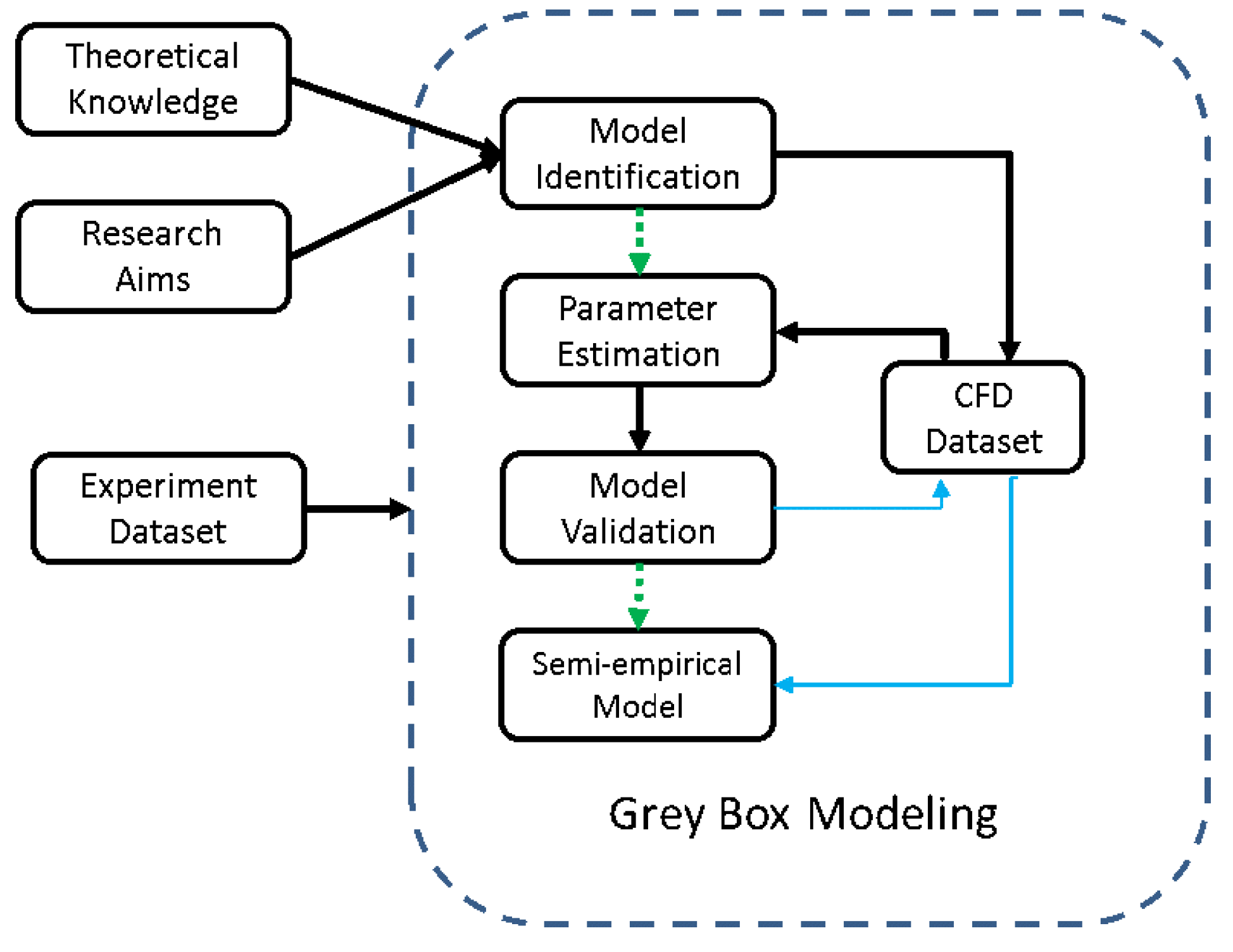
2.1. Grey Box Modeling

Various methods have been applied to an increasing number of complex physical systems, which also render the development and the quality of models [37]. A model has to be able to predict the future status of the system, and it should reveal its inherent behavior and provide ways to accommodate process or measurement noises due to approximation errors or imperfect measurements. Black box modeling satisfies the accommodating noise but fail to reveal the inherent behavior, while white box modeling achieves the opposite effects. Grey box modeling has the benefits of both aforementioned models and combine a partial theoretical structure with some undefined parameters [38]. The theoretical structure is derived from the theoretical formulations, and the parameter values need to be estimated from data or existing literature.

In this study, the air flow rate is set as the only target variable, and semi-empirical model is built based on the grey box modeling process shown in Figure 1. The key tasks are the identification of key independent variables, estimation of parameters and validation of the semi-empirical model.

2.1.1. Model Identification

The research aim is to develop a semi-empirical model to predict air flow rate in an atrium, as shown in Figure 1. Based on the assumption of Bruce’s neutral height-based formulation and combining it with the theoretical knowledge of Bernoulli’s equations and conservation equations of mass and energy, the model is identified with independent key factors of buoyancy-driven ventilation and deduction coefficients. Similarly to other general grey box models, this semi-empirical model is a non-linear model with a theoretical structure and some integrated parameters derived from data.

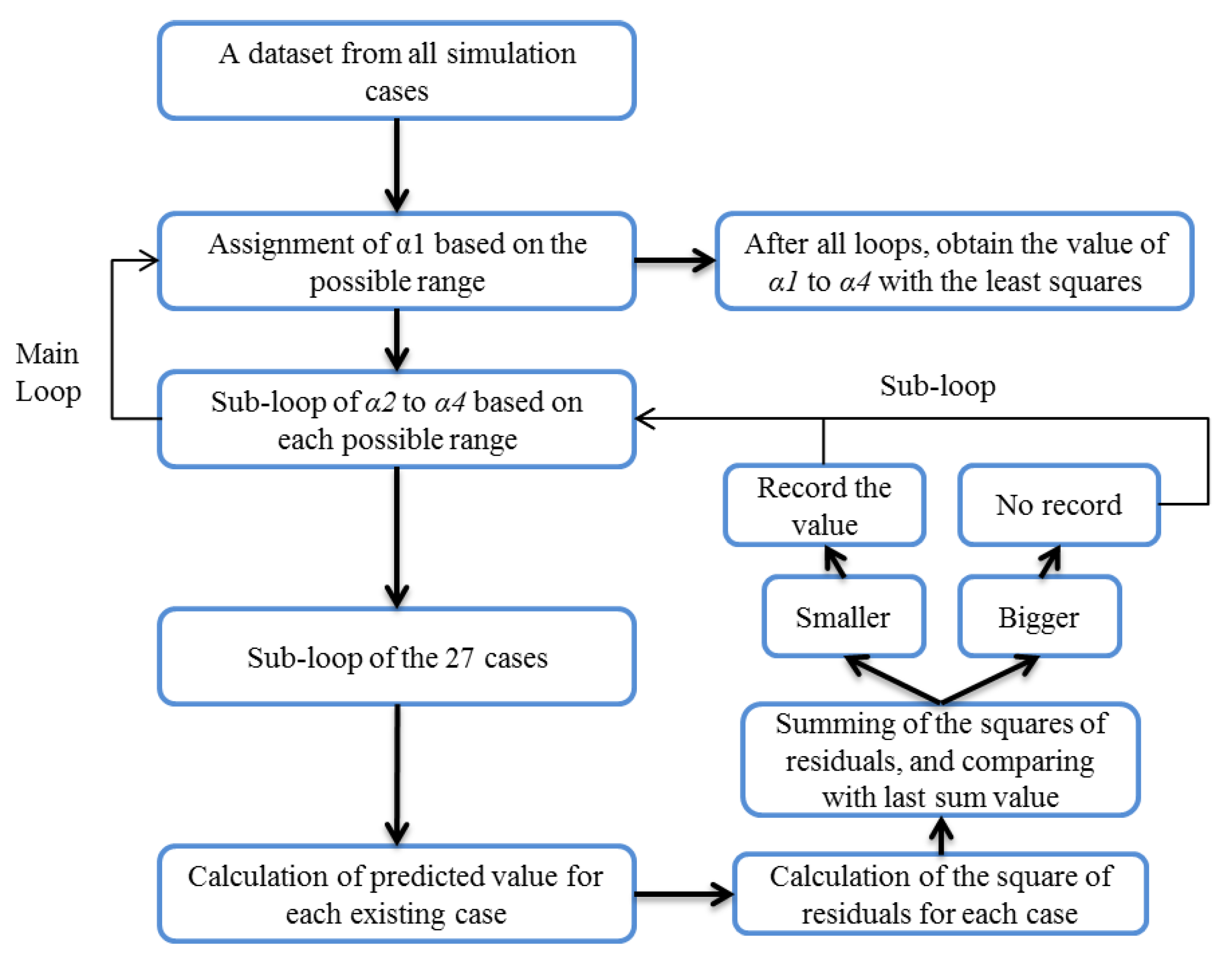
2.1.2. Parameters Estimation

Within a particular model structure, integrated parameters should be estimated with a series of groups of data, then the semi-empirical model could be established and have the capability of prediction. To obtain a series of data, a physical model was built based on a real building and its ventilation performance was calculated with a CFD model. Cases were defined with the principle of control variates method and variables were selected according to the key variables identified in last section.

The method of least squares was adopted to estimate parameters for weighting variables, and this method is a standard approach in regression analysis to minimize the sum of the squares of the residuals made in the results of every single equation. In this study, the semi-empirical model with two openings was identified with 2 integrated parameters for independent variables, while the model with three openings had 4 parameters. To estimate the values, a regression calculation was running with a Visual Studio program written by authors and the process illustrated with 4 parameters is shown as Figure 2.

2.1.3. Model Verification and Validation

The parameters can be obtained through fitting with either CFD simulation data or experimental data, and then the semi-empirical model is built. The semi-empirical model is then used to predict air flow rates in new cases. Therefore, this model would be evaluated in two aspects: first the error of the established model construction and second the prediction error for new cases. To testify the accuracy and rationality of this grey box modeling, more CFD simulation cases described in Section 4 were adopted to validate this method.

2.2. CFD Settings

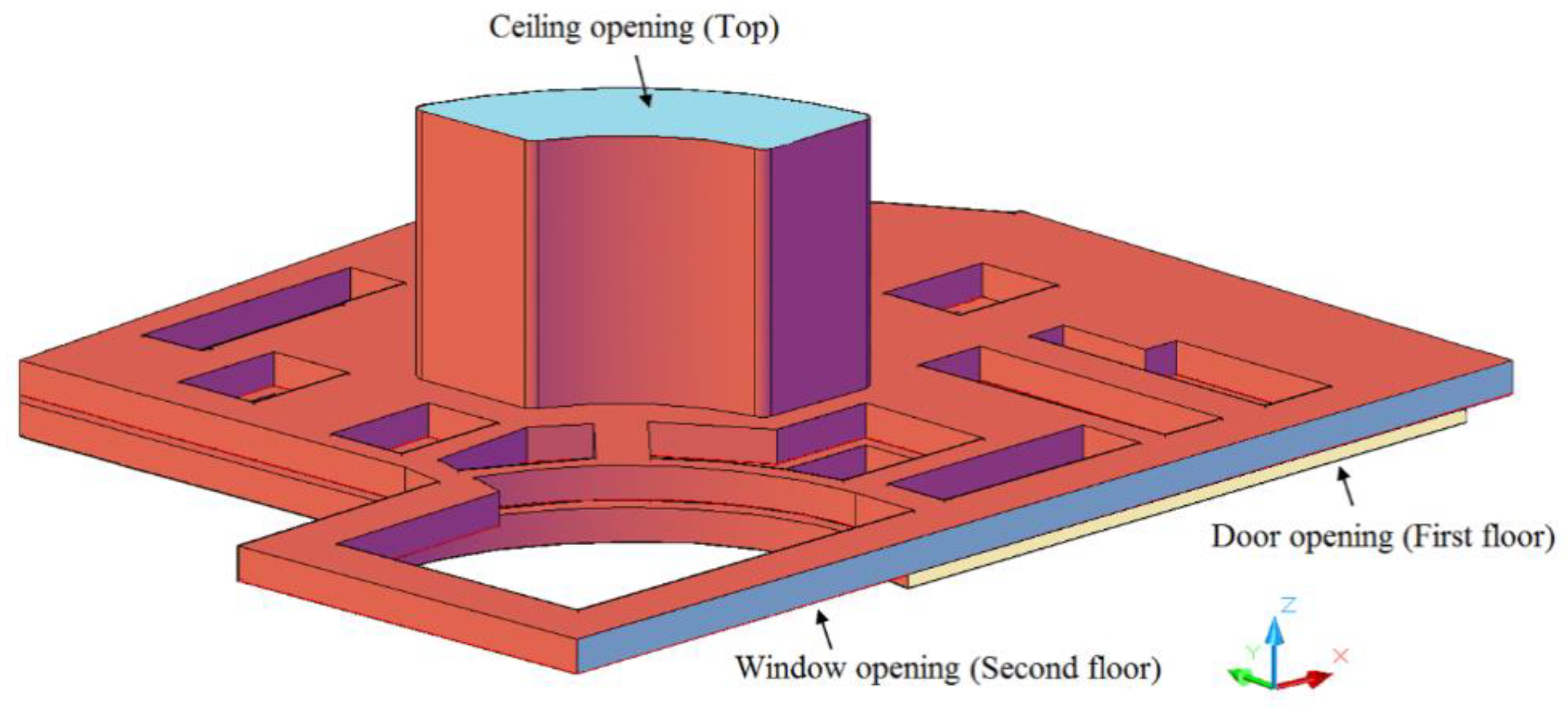
2.2.1. Physical Configuration

An atrium with three openings in design stage is selected to study the air flow rate based on grey box modeling method. The atrium is connected with several corridors in both the first and second floors, and corridors are connected to outside, as shown in Figure 3. The openable areas of doors and windows on the first and second floors are 774 m² and 2385 m² respectively. The area of the ceiling at the top of atrium is 838 m², the total floor area is 4860 m² and the heat flux of human and equipment are provided as 26.8 W/m² (light activity) and 25 W/m² respectively through the atrium floor with a uniform distribution [39]. Based on the data of typical meteorological year, the medium outdoor air temperature is 14 °C among two transition seasons (April~June, and September~November) with the building location.

2.2.2. Numerical Model and Boundary Conditions

Computational fluid dynamics is a technique that is able to calculate air flow rate in an efficient way. Compared with the Large Eddy Simulation (LES), Reynolds averaged Navier–Stokes equation (RANS) modeling requires much less computing time [40]. In the RANS framework, the two-equation turbulence models, namely, k-ε models, are very widely adopted. The corresponding governing transport equations for the k–ε turbulence models can be generalized as Equation (1):

$$\frac{\partial \left(\rho \Phi \right)}{\partial t}+div\left(\rho \stackrel{\rightharpoonup }{u}\Phi -{Г}_{\Phi ,eff}grad(\Phi )\right)=S_{\Phi }$$

(1)

where Ф represents the scalars: the velocity components, u, v, w, turbulent kinetic energy k and its dissipation rate ε; $\stackrel{\rightharpoonup }{u}$ is the time averaged velocity components; ρ is molecular density; Г is the diffusion coefficient, and S_Ф is the source term of Ф.

The exchange of air (bi-directional) through the atrium horizontal opening was predicted by CFD using the commercial software FLUENT. The computational domain was the whole atrium building, as shown in Figure 3. The grid for the atrium model consists of approximately 4,488,690 unstructured cells with high density cells arranged in the regions around the openings. This grid was selected after a sensitivity analysis of the cells number independence, which shows that further increasing the cells number leads to only slight changes to the predicted ventilation rates. The initial boundary conditions of openings were set as pressure inlet or outlet without pressure difference. The outdoor temperature was set based on typical meteorological year data. The wall surfaces were treated as a non-slip wall boundary condition, where the standard wall functions were applied. The empirical turbulence coefficients of the k-ε turbulence model were assigned as following values: C1 = 1.44, C2 = 1.92, Cµ = 0.09, σε = 1.3and σk = 1.0. The Boussinesq assumption was used to deal with the relationship between air density and air temperature. The PISO (Pressure Implicit with Splitting of Operators) algorithm was applied to calculate the pressure-velocity coupling, and the second-order upwind scheme was employed for the discretization of density, momentum and turbulent kinetic energy terms. Convergence of solutions was reached after the flow and temperature fields inside the atrium were stable.

3. Development of Grey Box Modeling

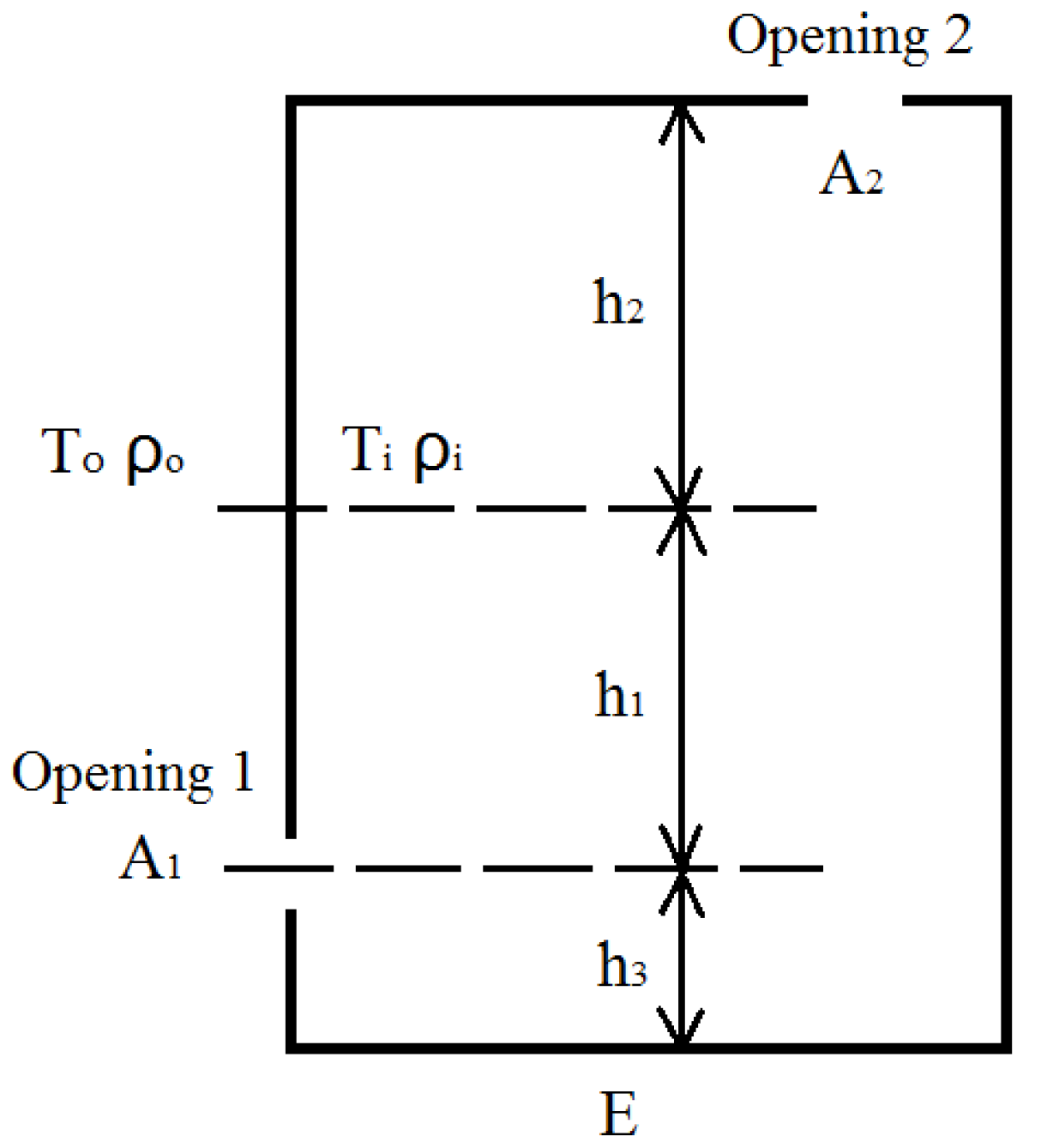
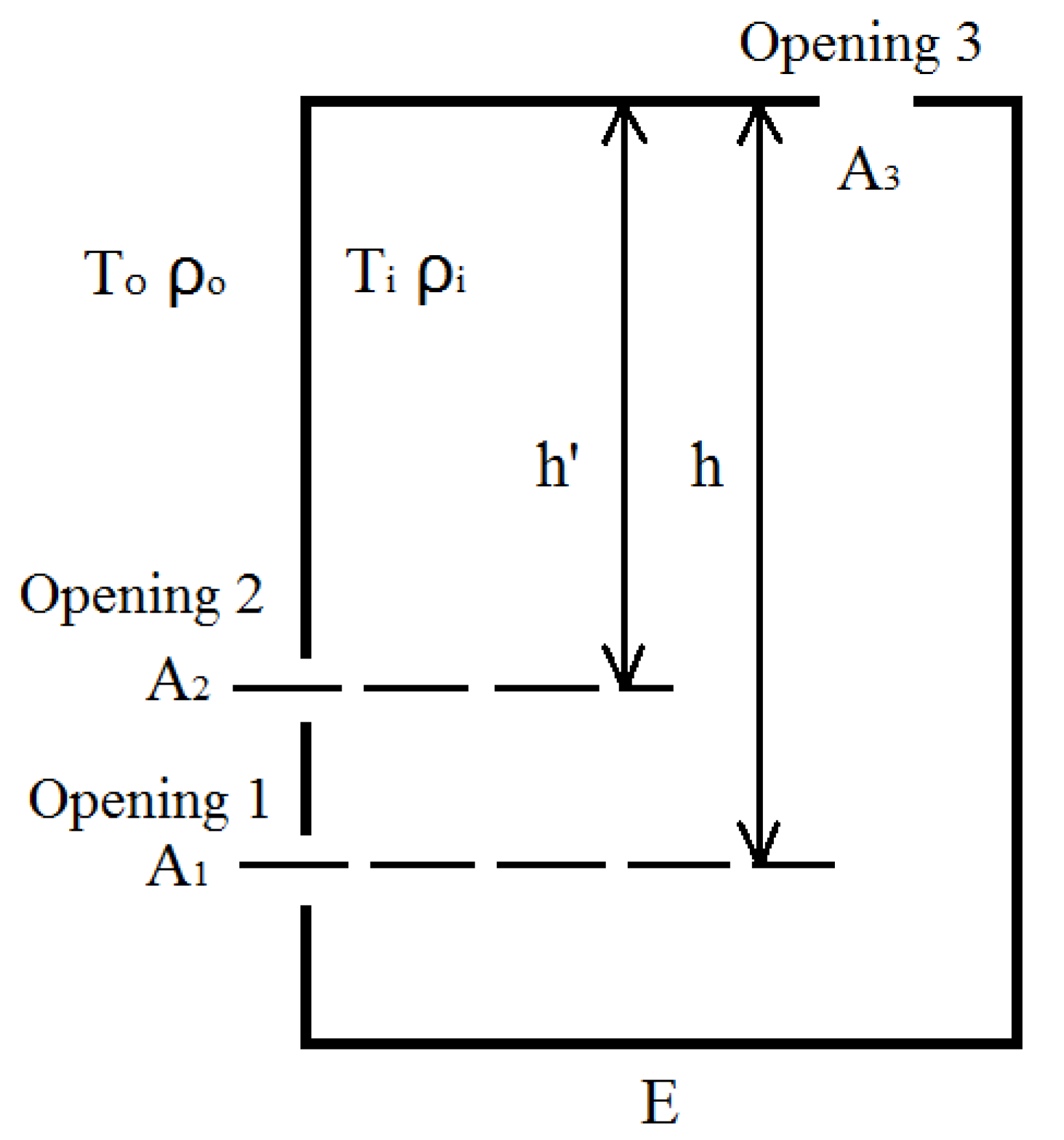
3.1. Two-Opening Model

The formulations are developed for a single-zone building with two openings, which are started with Bruce’s neutral height-based theory. The simplified model is shown in Figure 4. The heights between openings and the neutral plane are named as h₁ and h₂, while h stands for the height between the two openings. The relation (Figure 4) is shown as follows:

$$h=h_1+h_2$$

(2)

By assuming that the indoor air density is uniform, the pressure differences at openings can be calculated by solving a linear equation:

$$\Delta P_1=h_1\left({\rho }_o-{\rho }_i\right)g$$

(3)

$$\Delta P_2=h_2\left({\rho }_o-{\rho }_i\right)g$$

(4)

The Bernoulli equation can be applied on the flows across the openings:

$$v^2=\frac{2\Delta P}{\rho }$$

(5)

Although the air volume flow rates may be different at the inlet opening and the outlet opening due to the change of air density, the mass flow rates are the same:

$$M=M_1=M_2$$

(6)

The air mass flow rates at both openings can be written as:

$$M_1={\rho }_o{Q}_1={\rho }_o{A}_1{v}_1={\rho }_o{C}_{d1}{A}_1\sqrt{\frac{2\Delta P_1}{{\rho }_o}}$$

(7)

$$M_2={\rho }_i{Q}_2={\rho }_i{A}_2{v}_2={\rho }_i{C}_{d2}{A}_2\sqrt{\frac{2\Delta P_2}{{\rho }_i}}$$

(8)

where $A_1$ is the area of lower opening, $A_2$ is the area of upper opening, ${\rho }_o$ is the density of outdoor air, ${\rho }_i$ is the density of indoor air, $v_1$ is the air velocity through lower opening, $v_2$ is the air velocity through upper opening, $C_{d1}$ is the discharge coefficient for lower opening and $C_{d2}$ is the discharge coefficient for upper opening.

The discharge coefficient is a parameter for a specific aperture and includes both friction and contraction loss, which depends on the characteristics of both flow field and opening configuration.

Substituting Equation (3) into (7) and Equation (4) into (8), the mass flow rates can be obtained as:

$$M_1={\rho }_0{C}_{d1}{A}_1\sqrt{\frac{2h_1\left({\rho }_o-{\rho }_i\right)g}{{\rho }_o}}$$

(9)

$$M_2={\rho }_i{C}_{d2}{A}_2\sqrt{\frac{2h_2\left({\rho }_o-{\rho }_i\right)g}{{\rho }_i}}$$

(10)

In order to eliminate h₁ and h₂, the product of the square of the Equation (9) and $C_{d2}{}^2{A}_2{}^2{\rho }_i$ and the product of the square of the Equation (10) and $C_{d1}{}^2{A}_1{}^2{\rho }_o$ are summed and substituted into Equation (6):

$$\begin{array}{l}\left(C_{d2}{}^2{A}_2{}^2{\rho }_i+C_{d1}{}^2{A}_1{}^2{\rho }_o\right)M^2\\ \hspace{1em}\hspace{1em}\hspace{1em}\hspace{1em}\hspace{1em}\hspace{1em}\hspace{1em}\hspace{1em}=2C_{d1}{}^2{C}_{d2}{}^2{A}_1{}^2{A}_2{}^2{\rho }_o{\rho }_i\left({\rho }_o-{\rho }_i\right)g{h}_1\\ \hspace{1em}\hspace{1em}\hspace{1em}\hspace{1em}\hspace{1em}\hspace{1em}\hspace{1em}\hspace{1em}+2C_{d1}{}^2{C}_{d2}{}^2{A}_1{}^2{A}_2{}^2{\rho }_o{\rho }_i\left({\rho }_o-{\rho }_i\right)g{h}_2\\ \hspace{1em}\hspace{1em}\hspace{1em}\hspace{1em}\hspace{1em}\hspace{1em}\hspace{1em}\hspace{1em}=2C_{d1}{}^2{C}_{d2}{}^2{A}_1{}^2{A}_2{}^2{\rho }_o{\rho }_i\left({\rho }_o-{\rho }_i\right)gh\end{array}$$

(11)

In most natural ventilation conditions, the air is incompressible and the relationship between air density and air temperature can be approximately written as:

$$\frac{\left({\rho }_o-{\rho }_i\right)}{{\rho }_i}\approx \frac{\left(T_i-T_o\right)}{T_o}$$

(12)

where $T_o$ is the outdoor air temperature and $T_i$ is the indoor air temperature.

Deforming the Equation (11) and substituting Equation (12) into (11), the square of mass flow rate becomes:

$$M^2=2\frac{C_{d1}{}^2{C}_{d2}{}^2{A}_1{}^2{A}_2{}^2{\rho }_o{\rho }_i{}^2}{{\rho }_i{C}_{d2}{}^2{A}_2{}^2+{\rho }_o{C}_{d1}{}^2{A}_1{}^2}\frac{\left({\rho }_o-{\rho }_i\right)}{{\rho }_i}gh=2\frac{C_{d1}{}^2{C}_{d2}{}^2{A}_1{}^2{A}_2{}^2{\rho }_o{\rho }_i{}^2}{{\rho }_i{C}_{d2}{}^2{A}_2{}^2+{\rho }_o{C}_{d1}{}^2{A}_1{}^2}\frac{\left(T_i-T_o\right)}{T_o}gh$$

(13)

The indoor heat source heats the air and decreases its density. Based on the conservation of energy, the heat balance can be presented as:

$$E=c_{p}M\left(T_i-T_o\right)$$

(14)

where E is the uniform heat flux on the floor, and $c_p$ is air isobaric heat capacity. The equation can be deformed as:

$$M=\frac{E}{c_p\left(T_i-T_o\right)}$$

(15)

Multiplying Equation (15) with (13) obtains:

$$M^3=2\frac{C_{d1}{}^2{C}_{d2}{}^2{A}_1{}^2{A}_2{}^2{\rho }_o{\rho }_i{}^2}{{\rho }_i{C}_{d2}{}^2{A}_2{}^2+{\rho }_o{C}_{d1}{}^2{A}_1{}^2}\frac{Egh}{T_o{c}_p}$$

(16)

Then the air mass flow rate can be obtained as:

$$M={(\frac{2C_{d2}{}^2{\rho }_i{}^{2}g}{c_p}\frac{A_1{}^2{A}_2{}^2}{\frac{{\rho }_i}{{\rho }_o}\frac{C_{d2}{}^2}{C_{d1}{}^2}{A}_2{}^2+A_1{}^2}\frac{Eh}{T_o})}^{1/3}={(\frac{2C_{d2}{}^2{\rho }_i{}^{2}g}{c_p})}^{1/3}{(\frac{A_1{}^2{A}_2{}^2}{A_1{}^2+\frac{{\rho }_i}{{\rho }_o}\frac{C_{d2}{}^2}{C_{d1}{}^2}{A}_2{}^2}\frac{Eh}{T_o})}^{1/3}$$

(17)

Combining (8) with (17), the air volume outflow rate can be written as:

$$Q_2={(\frac{2C_{d2}{}^{2}g}{c_p{\rho }_i})}^{1/3}{(\frac{A_1{}^2{A}_2{}^2}{A_1{}^2+\frac{{\rho }_i}{{\rho }_o}\frac{C_{d2}{}^2}{C_{d1}{}^2}{A}_2{}^2}\frac{Eh}{T_o})}^{1/3}$$

(18)

Defining ${\alpha }_1={(\frac{2C_{d2}{}^{2}g}{c_p{\rho }_i})}^{1/3}$ and ${\alpha }_2=\frac{{\rho }_i}{{\rho }_o}\frac{C_{d2}{}^2}{C_{d1}{}^2}$, the air volume inflow rate can be obtained as:

$$Q_2={\alpha }_1{(\frac{A_1{}^2{A}_2{}^2}{A_1{}^2+{\alpha }_2{A}_2{}^2}\frac{Eh}{T_o})}^{1/3}$$

(19)

Equation (19) is the semi-empirical model of air flow rate, and it indicates that the air flow rate has the cube root relation with the boundary conditions. In general, this model is similar to the model (Equation (20)) developed by Jiang and Chen [22]. However, different from their model, two different opening areas and their relationship are investigated and given in the present new model. The structure of the present new model is also similar to that (Equation (21)) derived by Fitzgerald and Woods (2008), where two opening areas are integrated as a single effective value A*. However, in their model, the outdoor air temperature is not included. The innovation of this new model is that it considers all initial independent variables $\left(A_1,A_2,E,T_o,h\right)$ and 2 additional undefined integrated parameters, and its structure can be applied extensively to a multi-opening model.

$$Q=h{(\frac{Eg{C}_d{}^2{A}^2}{18\rho C_p\left(T_{out}+273.15\right)})}^{1/3}$$

(20)

$$V={(\frac{A^{*2}\left(H-h_B\right)g\alpha E}{\rho C_p})}^{1/3}$$

(21)

3.2. Multi-Opening Model

It is common to have more than two openings in real atriums, where the ventilation condition becomes more complicated than that of two openings. If we derive the formulations as the steps presented in last section, it will be found that the Equation (6) is no longer valid. This will lead to a problem that h₁, h₂ and h₃ could not be eliminated in Equation (11). As these parameters are not independent ones, the semi-empirical model for air flow rate could not be built in this way.

The advantage of grey box modeling is to build correct relations among variables with fuzzy parameters and solve them with accurate data. Considering opening 2 is lower than the neutral height (Figure 5), an assumption could be proposed, which is that part of opening 3 works as the outlet for opening 1 and the rest part works as the outlet for opening 2. The outlet area in opening 3 for opening 1 is $\beta$A₃ (0 < $\beta$ < 1), while the outlet for opening 2 is (1-$\beta$)A₃. Therefore, based on Equation (18), the air flow rate could be presented as:

$$Q_3={\alpha }_1{(\frac{{\beta }^2{A}_1{}^2{A}_3{}^2}{A_1{}^2+{\alpha }_2{\beta }^2{A}_3{}^2}\frac{Eh}{T_o})}^{1/3}+{\alpha }_3{(\frac{{\left(1-\beta \right)}^2{A}_2{}^2{A}_3{}^2}{A_2{}^2+{\alpha }_4{\left(1-\beta \right)}^2{A}_3{}^2}\frac{E{h}^{\prime }}{T_o})}^{1/3}$$

(22)

where h is the height between opening 1 and opening 3, and h′ the height between opening 2 and opening 3. To simplify the model, the solution can be presented as:

$$Q_3={\alpha }_1^{\prime }{(\frac{A_1{}^2{A}_3{}^2}{A_1{}^2+{\alpha }_2^{\prime }{A}_3{}^2}\frac{Eh}{T_o})}^{1/3}+{\alpha }_3^{\prime }{(\frac{A_2{}^2{A}_3{}^2}{A_2{}^2+{\alpha }_4^{\prime }{A}_3{}^2}\frac{E{h}^{\prime }}{T_o})}^{1/3}$$

(23)

where ${\alpha }_1^{\prime }={(\frac{2C_{d3}{}^2{\beta }^{2}g}{c_p{\rho }_i})}^{1/3}$, ${\alpha }_2^{\prime }=\frac{{\rho }_i}{{\rho }_o}\frac{{\beta }^2{C}_{d3}{}^2}{C_{d1}{}^2}$, ${\alpha }_4^{\prime }={(\frac{2C_{d3}{}^2{\left(1-\beta \right)}^{2}g}{c_p{\rho }_i})}^{1/3}$ and ${\alpha }_4^{\prime }=\frac{{\rho }_i}{{\rho }_o}\frac{{\left(1-\beta \right)}^2{C}_{d3}{}^2}{C_{d1}{}^2}$. The semi-empirical model for multi-opening (two flow inlets) is therefore built with 7 independent variables and 4 integrated parameters. Based on the expressions, the ranges of these parameters could be approximately estimated as: ${\alpha }_1^{\prime }$ = [0, 3], ${\alpha }_2^{\prime }$ = [0, 16], ${\alpha }_3^{\prime }$ = [0, 3], ${\alpha }_4^{\prime }$ = [0, 16].

4. CFD Verification of the Grey Box Modeling Method

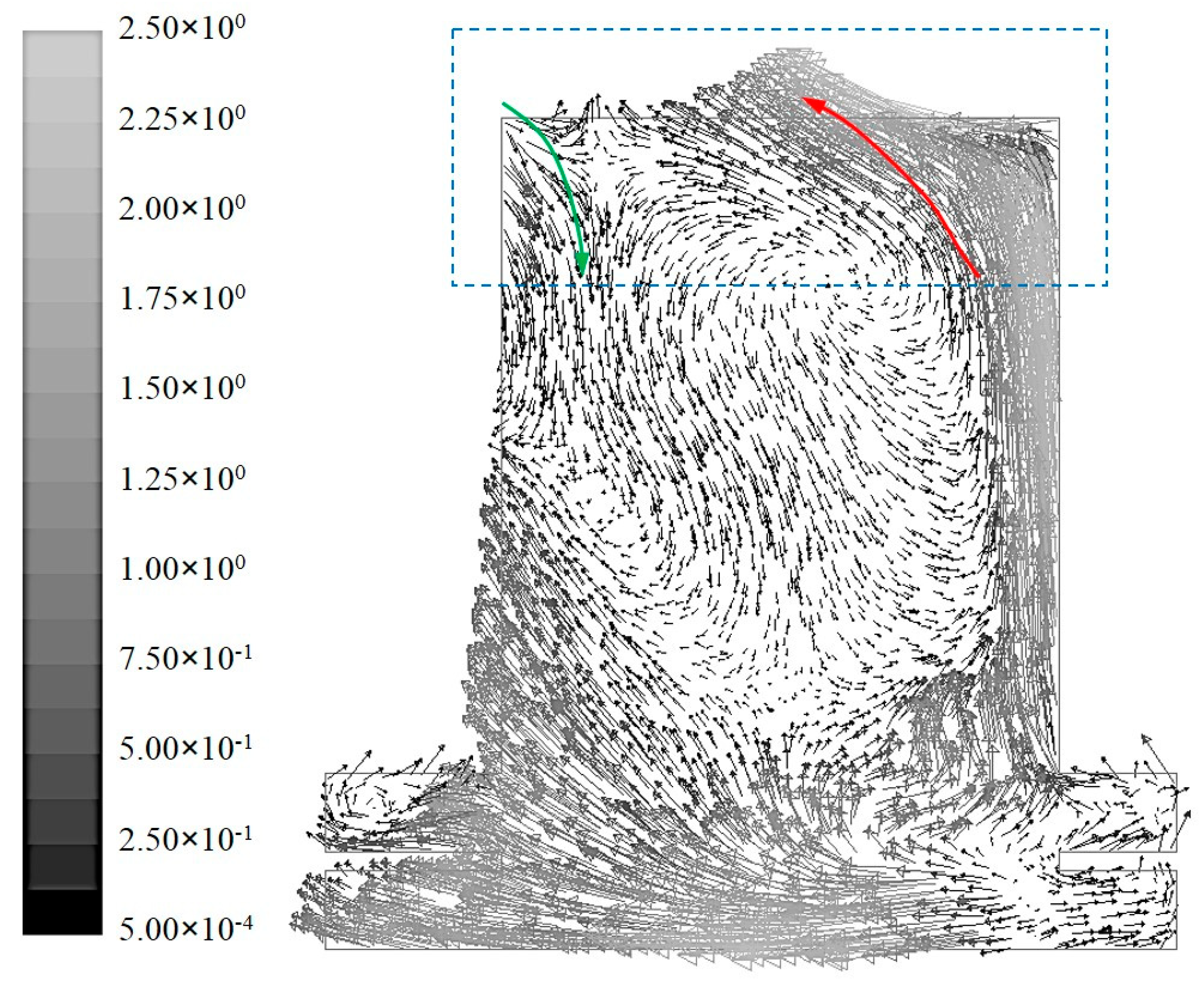
4.1. CFD Simulation Results

As shown in Section 2.2, 27 CFD cases were built to obtain the air flow rates under different conditions. Among all 7 independent variables, h and h′ were set as 19.6 m and 14.4 m respectively according to the real condition. Different values of other 5 variables were tested to study their influences on air flow rate. The results are shown in

Table 1. Summary of the simulation settings and results.

Case	Air Flow Rate (m3/s)	A1 (m2)	A2 (m2)	A3 (m2)	E (kJ/s)	To (K)	h (m)	h′ (m)
1-1	164	774	0	84 (10%)	252	287	19.6	none
1-2	224	774	0	168 (20%)	252	287	19.6	none
1-3(2-1)	239	774	0	251 (30%)	252	287	19.6	none
1-4	260	774	0	336 (40%)	252	287	19.6	none
1-5	276	774	0	419 (50%)	252	287	19.6	none
1-6	282	774	0	587(70%)	252	287	19.6	none
2-2	268	774	239(10%)	251 (30%)	252	287	19.6	14.4
2-3(3-5,4-2)	271	774	477(20%)	251 (30%)	252	287	19.6	14.4
2-4	275	774	716(30%)	251 (30%)	252	287	19.6	14.4
2-5	274	774	954(40%)	251 (30%)	252	287	19.6	14.4
2-6	272	774	1193(50%)	251 (30%)	252	287	19.6	14.4
3-1	140	155(20%)	477(20%)	251 (30%)	252	287	19.6	14.4
3-2	162	232(30%)	477(20%)	251 (30%)	252	287	19.6	14.4
3-3	185	310(40%)	477(20%)	251 (30%)	252	287	19.6	14.4
3-4	217	387(50%)	477(20%)	251 (30%)	252	287	19.6	14.4
4-1	293	774	477(20%)	251 (30%)	291	287	19.6	14.4
4-3	263	774	477(20%)	251 (30%)	218	287	19.6	14.4
4-4	251	774	477(20%)	251 (30%)	199	287	19.6	14.4
5-1	327	774	716(30%)	419 (50%)	252	283	19.6	14.4
5-2	326	774	716(30%)	419 (50%)	252	285	19.6	14.4
5-3	325	774	716(30%)	419 (50%)	252	287	19.6	14.4
5-4	322	774	716(30%)	419 (50%)	252	289	19.6	14.4
5-5	319	774	716(30%)	419 (50%)	252	291	19.6	14.4
5-6	317	774	716(30%)	419 (50%)	252	293	19.6	14.4
5-7	316	774	716(30%)	419 (50%)	252	295	19.6	14.4
5-8	312	774	716(30%)	419 (50%)	252	297	19.6	14.4
5-9	310	774	716(30%)	419 (50%)	252	299	19.6	14.4

.

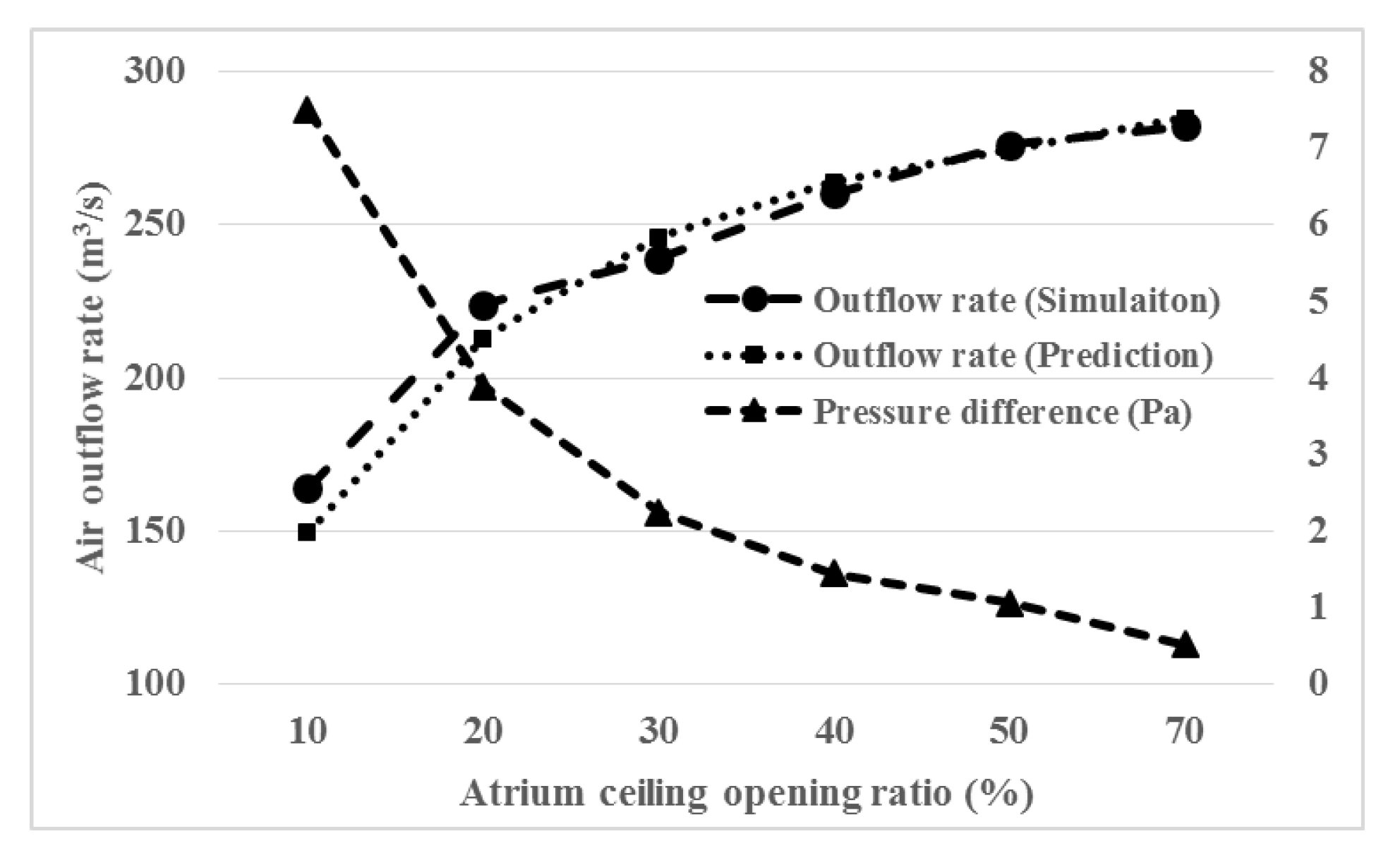
4.1.1. Influence of Ceiling Opening Area A₃

As seen from Table 1, six cases were designed to test the influence of ceiling opening area on the air outflow rate. All cases are set with 100% door opening on the first floor, no window opening on the second floor, 252 kJ/s indoor heat generation and 14 ℃ outdoor air temperature. With the increase of the opening from 10% to 70%, the air outflow rate increases from 164 m³/s to 282 m³/s, but the increasing rate drops gradually with the increase of the opening. To investigate this phenomenon, details of the air flow field are examined and provided in Figure 6.

With the increase of the opening, the pressure difference drops dramatically from 7.5 to 0.5 Pa, which leads to a gradually slower increase in the outflow rate. As seen from Figure 7, the low pressure difference also results in a certain amount of cold air entering the atrium from the ceiling opening. This part of cold air has a heat exchange with warm air before flowing out again from the ceiling opening. The ventilation at top opening becomes a bi-directional air flow after the opening increases to a certain area, which forms a bottleneck of the increase of the air outflow rate. In other words, solely enlarging the top opening area is not always an effective way to increase the air flow rate of an atrium.

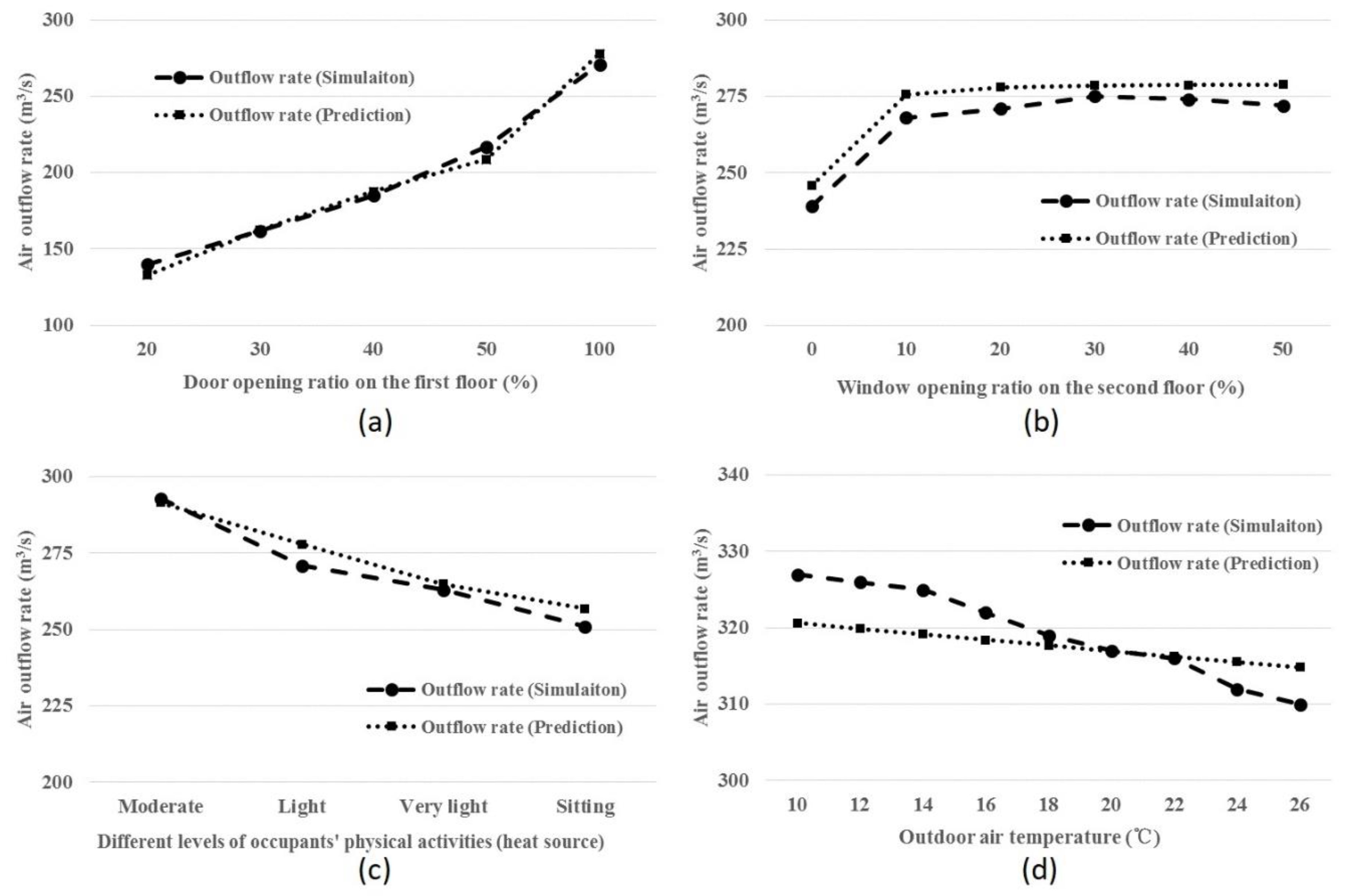
4.1.2. Influence of Door Opening Area A₁

Five cases were built to examine the influence of door opening area on air outflow rate, when the window opening ratio of the second floor was set to be 20%, ceiling opening was set to 30%, the total indoor heat flux was 252 kJ/s and outdoor air temperature was 14 ℃. With the increase of the door opening ratio from 20% to 100%, the air outflow rate increases from 140 m³/s to 271 m³/s (Figure 8a). This may indicate that the opening area at the lower (first) level is a key factor influencing the ventilation performance.

4.1.3. Influence of Window Opening Area A₂

Six cases were built to test the influence of the window opening ratio of the second floor on air outflow rate, when the door opening of the first floor was set as 100%, the ceiling opening at the top was 30%, total indoor heat flux was 252 kJ/s and outdoor air temperature was 14 ℃. The opening of the window of the second floor by 10% results in a sharp increase of air outflow rate by 25 m³/s. However, the flow rate changes slightly with the opening changing from 10% to 50% (Figure 8b). It may be indicated that the ventilation performance quickly reaches a balance status after opening the window, and the air flow rate in atrium does not change obviously with a further increase of window opening area.

4.1.4. Influence of Heat Source E

Referring to the Practical Heating and Air Conditioning Design Handbook of China, the total indoor heat power at four different levels of occupants’ physical activities were calculated, as shown in

Table 2. Total indoor heat power at different levels of occupants’ physical activities.

Activity	Body Heat Emission (W/p)	Coefficient of Community	Occupant Density (m2/p)	Equipment Load (W/m2)	Floor Area (m2)	Total Heat (kW)
Moderate	235	0.89	6	25	4860	291
Light	181					252
Very light	134					218
Sitting	108					199

.

All these 4 cases with different indoor heat fluxes were set with 100% door opening of the first floor, 20% window opening of the second floor, 30% ceiling opening at the top, and 14 ℃ outdoor air temperature. With the decrease of heat power from 291 kW to 199 kW, the air outflow rate decreases from 293 m³/s to 251 m³/s (Figure 8c). The relation between heat power and air outflow rate is almost linear and significant, which proves that the heat source in an atrium is also a key factor influencing the ventilation performance.

4.1.5. Influence of Outdoor Air Temperature T_o

As shown in Table 1, nine cases were designed to examine the influence of outdoor air temperature on the air flow rate in atrium. All cases were set with 100% door opening of the first floor, 30% window opening of the second floor, 50% ceiling opening at the top, and 252 kJ/s total heat. As shown in Figure 8d, with the increase of outdoor air temperature from 10 ℃ to 26 ℃, which leads to a decrease of indoor/outdoor pressure difference, the air outflow rate decreases from 327 m³/s to 310 m³/s. The results show that, although the buoyancy-driven natural ventilation is affected by the outdoor air temperature, the air flow rate can be kept at a relatively high level with certain opening designs and indoor heat sources.

4.2. Solutions of the Grey Box Model and Its Accuracy

Referring to the semi-empirical model as shown in Equation (23), the solutions of integrated parameters were computed using Visual Studio with the data obtained above. As there are 4 parameters, 5 loops are embedded in the programming process (see Figure 2). The test values of the parameters are restricted within certain ranges (calculated in Section 3.2) to reduce the calculation time, while the iterative target is to minimize the sum of the squares of the residuals of every single case. After the iteration, solutions of these parameters are obtained as ${\alpha }_1^{\prime }$ = 3.157, ${\alpha }_2^{\prime }$ = 12.335, ${\alpha }_3^{\prime }$ = 0.358, ${\alpha }_4^{\prime }$ = 0.337, with the sum of the squares of the residuals equals to 920.29. Therefore, the semi-empirical model of the air flow rate due to the buoyancy effect comes as:

$$Q=3.157{(\frac{A_1{}^2{A}_3{}^2}{A_1{}^2+12.335A_3{}^2}\frac{Eh}{T_o})}^{1/3}+0.358{(\frac{A_2{}^2{A}_3{}^2}{A_2{}^2+0.337A_3{}^2}\frac{E{h}^{\prime }}{T_o})}^{1/3}$$

(24)

Prediction values in each case could be calculated by this equation and the comparison of air flow rates between CFD simulation and semi-empirical prediction is shown in Figure 6 and Figure 8 within different groups. The largest residual happens in the first case with a rather small ceiling opening, where the error is 8.89%. In other 26 cases, the errors are less than 5% (

Table 3. Comparison of air flow rates between CFD simulation and semi-empirical prediction.

Case	Simulated Value (m3/s)	Prediction Value (m3/s)	Square of Residual	Error
1-1	164	149.42	212.52	8.89%
1-2	224	213.02	120.61	4.90%
1-3(2-1)	239	245.80	46.25	−2.85%
1-4	260	263.95	15.57	−1.52%
1-5	276	274.13	3.49	0.68%
1-6	282	284.59	6.73	−0.92%
2-2	268	275.67	58.81	−2.86%
2-3(3-5,4-2)	271	278.01	49.20	−2.59%
2-4	275	278.54	12.54	−1.29%
2-5	274	278.73	22.40	−1.73%
2-6	272	278.82	46.56	−2.51%
3-1	140	132.98	49.33	5.02%
3-2	162	162.47	0.22	−0.29%
3-3	185	187.64	6.95	−1.43%
3-4	217	208.86	66.19	3.75%
4-1	293	291.67	1.76	0.45%
4-3	263	264.90	3.62	−0.72%
4-4	251	256.97	35.66	−2.38%
5-1	327	320.66	40.22	1.94%
5-2	326	319.91	37.13	1.87%
5-3	325	319.16	34.09	1.80%
5-4	322	318.42	12.79	1.11%
5-5	319	317.69	1.71	0.41%
5-6	317	316.97	0.00	0.01%
5-7	316	316.25	0.06	−0.08%
5-8	312	315.54	12.52	−1.13%
5-9	310	314.83	23.36	−1.56%

), which indicates that this semi-empirical prediction model is well curve fitted.

4.3. Sensitivity Analysis

The effects of set values of each parameter on air flow rate are shown in Figure 6 and Figure 8. Besides, the slope of air flow rate as a function of individual parameter can be used as a measure of how sensitive the air flow rate is to the particular parameter. The influence of each parameter on the air flow rate can be quantified by calculating the maximum variation of air flow rate caused by the parameter change of 0.01.

As shown in

Table 4. The maximum change in air flow rate caused by a parameter change of 0.01.

	A1 (m2)	A2 (m2)	A3 (m2)	E (kJ/s)	To (K)	h (m)	h′ (m)
Air flow rate	0.0008	0.0000	0.0059	0.0033	−0.0033	0.0030	0.0003

, the air flow rate is most sensitive to the ceiling opening area. That is, when these parameters change the same amount, the ceiling opening area will cause the biggest positive change to the air flow rate. The heat source also has a big positive change on the air flow rate, while the outdoor air temperature has a big negative effect. The total height of the whole atrium also has a significant impact on the air flow rate.

4.4. Prediction Accuracy of the Grey Box Model

In order to further assess the accuracy of the semi-empirical model, new cases were built for verification. Referring to the 5 changeable variables in the target atrium, 6 related cases are designed (as shown in

Table 5. Settings and results of new cases for further verification of the proposed model.

Case	A1 (m2)	A2 (m2)	A3 (m2)	E (kJ/s)	To (K)	h (m)	h′ (m)	Simulated Value (m3/s)	Predicted Value (m3/s)	Error
6-1	387 (50%)	716 (30%)	168 (20%)	199	289	19.6	14.4	172.55	176.61	−2.35%
6-2	744 (100%)	716 (30%)	168 (20%)	199	289	19.6	14.4	223.18	217.77	2.42%
6-3	744 (100%)	954 (40%)	168 (20%)	199	289	19.6	14.4	222.36	217.83	2.04%
6-4	744 (100%)	954 (40%)	419 (50%)	199	289	19.6	14.4	275.31	289.76	−5.25%
6-5	744 (100%)	954 (40%)	419 (50%)	218	289	19.6	14.4	303.78	298.70	1.67%
6-6	744(100%)	954(40%)	419 (50%)	218	293	19.6	14.4	301.52	297.34	1.39%

) and the calculation results are also provided in the same table.

As seen from Table 5, the errors are all less than 6%, which indicates that the semi-empirical prediction is as accurate as the CFD simulation. Based on this verified semi-empirical model, optimization of the ventilation performance of the atrium is analyzed for a specific case in Section 5.1.

4.5. Computing Time Saving

CFD simulation of full-scale atrium buildings that involve coupled indoor and outdoor environments is extremely time consuming. This is particularly the case during the design stage when parametric studies are required to compare many cases. With the current acceptably accurate semi-empirical prediction model, CFD simulation is required for only a limited number of cases and the computing time for more cases can be saved. Moreover, the largest air flow rate can be easily determined and the optimal opening design with the expected flow rate can be obtained.

5. Discussion

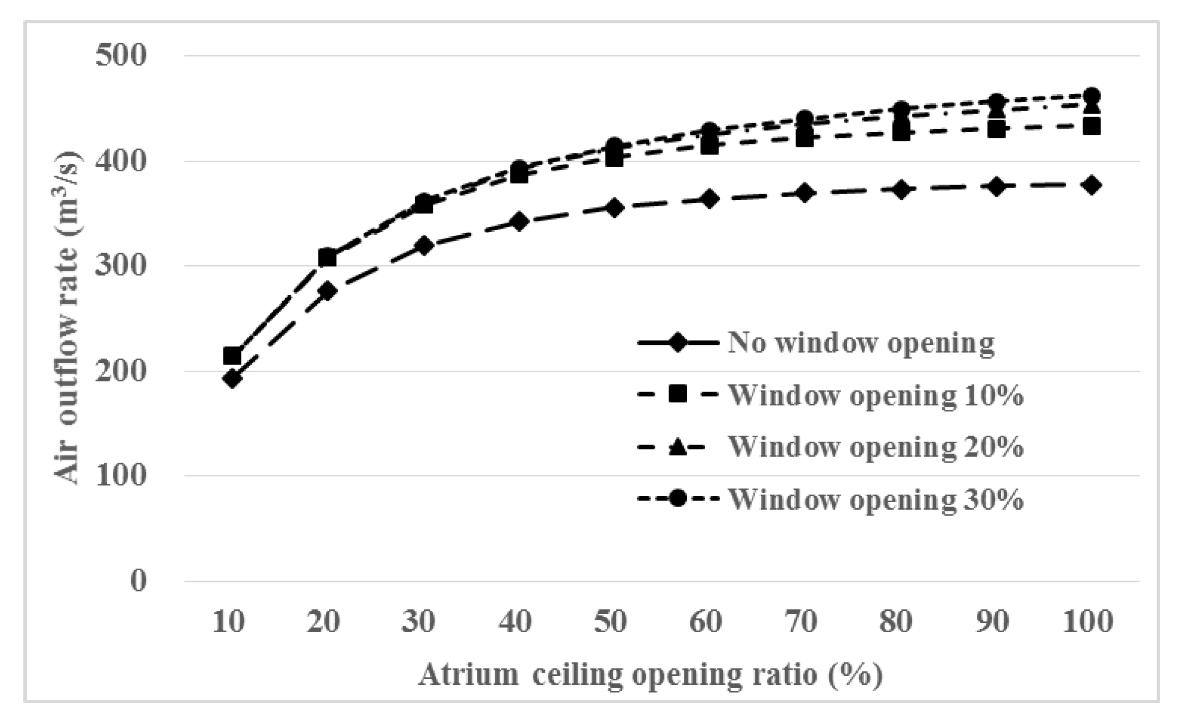
5.1. Maximizing the Air Flow Rate—A Case Study

With the specific prediction equation, the largest air flow rate could be estimated with a certain combination of influencing variables. Among others, if the heat source is stronger, the buoyance force will be enhanced, which leads to a larger air flow rate. Here comes a question that could the natural ventilation replace mechanical ventilation under the circumstance of a fire? Results from a series of tests with plywood show the flame heat flux ranges from 5 to 10 kW/m² [41]. In the atrium discussed in Section 4, if the area of a fire is 40 m², the total indoor heat flux would become 552 kJ/s with an increase of 300 kJ/s from the original total heal flux. In a real condition, if E = 552 kJ/s, T_o = 14 °C, h = 19.6 m and h′ = 14.4 m, the largest air flow rate could be reached when the door is fully opened (100%). Keeping the door opening as 100%, the relationship of air outflow rate through the atrium with other two variables, namely window opening and ceiling opening can be predicted, as shown in Figure 9.

It can be seen from the figure that, in order to maximize air flow rate, opening the window is needed, but the opening area does not need to be very large as there is no much difference produced by the different opening areas from 10% to 30%. In addition, the change of air flow rate tends to be gentle when the ceiling opening ratio becomes larger than 60%. Based on these results, the optimal control mode under fire conditions is to open all doors, open 10% of the window, open 60% of the ceiling, and then the air flow rate could reach 415 m³/s. In this case, the air exchange rate is approximately 16 times/hour. Given that the requirement of emergency ventilation is 12 times/hour [42], the above calculation may indicate that buoyancy-driven natural ventilation can be used to replace mechanical ventilation under some circumstances.

5.2. Limitations

Two limitations can be identified in our analysis. The first one is attached to the independent variables. In the process of parameters estimation with simulated data, h and h′ were constants in all cases according to the real building plan. If all these seventh independent variables were tested as non-constants during the process of parameters estimation, the semi-empirical model should be more accurate for predicting air flow rates. The second limitation is the application of the model. Based on the grey box modeling, the prediction method can be used extensively to other buildings, but the parameters of the predictive equation obtained for one type of building may not be the same as another. In the future, the factors affecting integrated parameters should be investigated and a simple method for estimating parameters should be developed.

6. Conclusions

In this study, a grey box modeling method is proposed to predict buoyancy-driven air flow rate in an atrium building with three openings. This model is developed from Bruce’s neutral height-based formulation and conservation laws. The model is identified with a theoretical structure and equipped with 4 integrated parameters and 7 independent variables, namely the areas of three openings, heat flux, outdoor air temperature, and the heights between ceiling opening with the other two lower openings. The lower opening area is found to be the key factor affecting the air flow rate. The integrated parameters could be estimated from a quite small simulated dataset. With the estimated parameters, a semi-empirical model is established for predicting the air flow rate. In this study, the error of the prediction equation derived from CFD (computational fluid dynamics) simulated data is controlled within 10%. This modeling method has been validated with CFD simulation, and can be applied extensively to similar buildings for designing an expected ventilation rate. This proposed simple method saves much computing time for designers on estimating the ventilation performance and helps to choose the best openings arrangement for façade and roof design.

References

1. Aflaki, A.; Mahyuddin, N.; Al-Cheikh Mahmoud, Z.; Baharum, M.R. A review on natural ventilation applications through building façade components and ventilation openings in tropical climates. Energy Build. 2015, 101 (Suppl. C), 153–162. [Google Scholar] [CrossRef]
2. Awbi, H.B. Air movement in naturally-ventilated buildings. Renew. Energy 1996, 8, 241–247. [Google Scholar] [CrossRef]
3. Khoshbakht, M.; Gou, Z.; Xie, X.; He, B.; Darko, A. Green Building Occupant Satisfaction: Evidence from the Australian Higher Education Sector. Sustainability 2018, 10, 2890. [Google Scholar] [CrossRef]
4. Alibaba, H.Z. Heat and Air Flow Behavior of Naturally Ventilated Offices in a Mediterranean Climate. Sustainability 2018, 10, 3284. [Google Scholar] [CrossRef]
5. Awbi, H.B. Ventilation of Buildings; Routledge: Abingdon, UK, 2002. [Google Scholar]
6. Chen, Z.D.; Li, Y. Buoyancy-driven displacement natural ventilation in a single-zone building with three-level openings. Build. Environ. 2002, 37, 295–303. [Google Scholar] [CrossRef]
7. Favarolo, P.A.; Manz, H. Temperature-driven single-sided ventilation through a large rectangular opening. Build. Environ. 2005, 40, 689–699. [Google Scholar] [CrossRef]
8. Omrani, S.; Garcia-Hansen, V.; Capra, B.; Drogemuller, R. Natural ventilation in multi-storey buildings: Design process and review of evaluation tools. Build. Environ. 2017, 116, 182–194. [Google Scholar] [CrossRef] [Green Version]
9. Gao, J.; Zhao, J.N.; Gao, F.S.; Zhang, X. Modeling of Indoor Thermally Stratified Flows on the Basis of Eddy Viscosity/Diffusivity Model: State of the Art Review. J. Build. Phys. 2009, 32, 221–241. [Google Scholar]
10. Ji, Y.; Cook, M.J.; Hanby, V. CFD modeling of natural displacement ventilation in an enclosure connected to an atrium. Build. Environ. 2007, 42, 1158–1172. [Google Scholar] [CrossRef]
11. Li, Y.; Delsante, A.; Symons, J. Prediction of natural ventilation in buildings with large openings. Build. Environ. 2000, 35, 191–206. [Google Scholar] [CrossRef]
12. Linden, P.; Lane-Serff, G.; Smeed, D. Emptying filling boxes: The fluid mechanics of natural ventilation. J. Fluid Mech. 1990, 212, 309–335. [Google Scholar] [CrossRef]
13. Fitzgerald, S.D.; Woods, A.W. Natural ventilation of a room with vents at multiple levels. Build. Environ. 2004, 39, 505–521. [Google Scholar] [CrossRef]
14. Gao, J.; Gao, F.-S.; Zhao, J.-N.; Liu, J. Calculation of Natural Ventilation in Large Enclosures. Indoor Built Environ. 2007, 16, 292–301. [Google Scholar] [CrossRef]
15. Hayden, C.S.; Earnest, G.S.; Jensen, P.A. Development of an Empirical Model to Aid in Designing Airborne Infection Isolation Rooms. J. Occup. Environ. Hyg. 2007, 4, 198–207. [Google Scholar] [CrossRef] [PubMed]
16. Kotani, H.; Satoh, R.; Yamanaka, T. Natural ventilation of light well in high-rise apartment building. Energy Build. 2003, 35, 427–434. [Google Scholar] [CrossRef]
17. O’Sullivan, P.D.; Kolokotroni, M. A field study of wind dominant single sided ventilation through a narrow slotted architectural louvre system. Energy Build. 2017, 138, 733–747. [Google Scholar] [CrossRef]
18. Allocca, C.; Chen, Q.; Glicksman, L.R. Design analysis of single-sided natural ventilation. Energy Build. 2003, 35, 785–795. [Google Scholar] [CrossRef]
19. Ai, Z.T.; Mak, C.M. Analysis of fluctuating characteristics of wind-induced airflow through a single opening using LES modeling and the tracer gas technique. Build. Environ. 2014, 80, 249–258. [Google Scholar] [CrossRef]
20. Ai, Z.T.; Mak, C.M.; Niu, J.L.; Li, Z.R. Effect of balconies on thermal comfort in wind-induced, naturally ventilated low-rise buildings. Build. Serv. Eng. Res. Technol. 2011, 32, 277–292. [Google Scholar] [CrossRef]
21. Ai, Z.T.; Mak, C.M. Determination of single-sided ventilation rates in multistory buildings: Evaluation of methods. Energy Build. 2014, 69, 292–300. [Google Scholar] [CrossRef]
22. Jiang, Y.; Chen, Q. Buoyancy-driven single-sided natural ventilation in buildings with large openings. Int. J. Heat Mass Transf. 2003, 46, 973–988. [Google Scholar] [CrossRef]
23. Olenets, M.; Piotrowski, J.Z. A model of heat and air transfer in a ventilated, rectangular space. J. Build. Phys. 2017, 40, 334–345. [Google Scholar] [CrossRef]
24. Heiselberg, P.; Svidt, K.; Nielsen, P.V. Characteristics of airflow from open windows. Build. Environ. 2001, 36, 859–869. [Google Scholar] [CrossRef]
25. Arendt, K.; Krzaczek, M.; Tejchman, J. Influence of input data on airflow network accuracy in residential buildings with natural wind- and stack-driven ventilation. Build. Simul. 2017, 10, 229–238. [Google Scholar] [CrossRef]
26. Van Hooff, T.; Blocken, B. Coupled urban wind flow and indoor natural ventilation modeling on a high-resolution grid: A case study for the Amsterdam ArenA stadium. Environ. Model. Softw. 2010, 25, 51–65. [Google Scholar] [CrossRef]
27. Wang, H.; Karava, P.; Chen, Q. Development of simple semiempirical models for calculating airflow through hopper, awning, and casement windows for single-sided natural ventilation. Energy Build. 2015, 96 (Suppl. C), 373–384. [Google Scholar] [CrossRef]
28. Keig, P.; Hyde, T.; McGill, G. A comparison of the estimated natural ventilation rates of four solid wall houses with the measured ventilation rates and the implications for low-energy retrofits. Indoor Built Environ. 2016, 25, 169–179. [Google Scholar] [CrossRef]
29. Gullbrekken, L.; Uvsløkk, S.; Geving, S.; Kvande, T. Local loss coefficients inside air cavity of ventilated pitched roofs. J. Build. Phys. 2017, 42, 197–219. [Google Scholar] [CrossRef] [Green Version]
30. Gan, G. Simulation of buoyancy-induced flow in open cavities for natural ventilation. Energy Build. 2006, 38, 410–420. [Google Scholar] [CrossRef]
31. Bouzinaoui, A.; Vallette, P.; Lemoine, F.; Fontaine, J.R.; Devienne, R. Experimental study of thermal stratification in ventilated confined spaces. Int. J. Heat Mass Transf. 2005, 48, 4121–4131. [Google Scholar] [CrossRef]
32. Ji, J.; Gao, Z.H.; Fan, C.G.; Sun, J.H. Large Eddy Simulation of stack effect on natural smoke exhausting effect in urban road tunnel fires. Int. J. Heat Mass Transf. 2013, 66 (Suppl. C), 531–542. [Google Scholar] [CrossRef]
33. Heiselberg, P.; Li, Z. Buoyancy Driven Natural Ventilation through Horizontal Openings. Int. J. Vent. 2009, 8, 219–231. [Google Scholar] [CrossRef] [Green Version]
34. Chen, Q. Ventilation performance prediction for buildings: A method overview and recent applications. Build. Environ. 2009, 44, 848–858. [Google Scholar] [CrossRef]
35. Wu, P.; Feng, Z.; Cao, S.-J. Fast and accurate prediction of airflow and drag force for duct ventilation using wall-modeled large-eddy simulation. Build. Environ. 2018, 141, 226–235. [Google Scholar] [CrossRef]
36. Bruce, J.M. Natural convection through openings and its application to cattle building ventilation. J. Agric. Eng. Res. 1978, 23, 151–167. [Google Scholar] [CrossRef]
37. Kristensen, N.R.; Madsen, H.; Jørgensen, S.B. Parameter estimation in stochastic grey-box models. Automatica 2004, 40, 225–237. [Google Scholar] [CrossRef]
38. Kroll, A. Grey-box models: Concepts and application. In New Frontiers in Computational Intelligence and its Applications; Ios Pr Inc.: Washington, DC, USA, 2000; Volume 57, pp. 42–51. [Google Scholar]
39. Lu, Y.-Q. Handbook of Practical Heating and Air Conditioning Design; China Architecture & Building Press: Beijing, China, 2008. [Google Scholar]
40. Cao, S.-J.; Meyers, J. Asymptotic conditions for the use of linear ventilation models in the presence of buoyancy forces. Build. Simul. 2014, 7, 131–136. [Google Scholar] [CrossRef]
41. Delichatsios, M.; Wu, P.; Delichatsios, M.; Lougheed, G.; Crampton, G.; Qian, C.; Lshida, H.; Saito, K. Effect of external radiant heat flux on upward fire spread: Measurements on plywood and numerical predictions. Fire Saf. Sci. 1994, 4, 421–432. [Google Scholar] [CrossRef]
42. GB 50736. Design Code for Heating Ventilation and Air Conditioning of Civil Buildings; China Architecture & Building Press: Beijing, China, 2012. [Google Scholar]
Figure 1. Grey box modeling for predicting air flow rate.
Sustainability 11 03239 g001
Figure 2. Logic diagram for estimating integrated parameters.
Sustainability 11 03239 g002
Figure 3. Physical model of the target atrium.
Sustainability 11 03239 g003
Figure 4. Independent variables in a two-opening atrium.
Sustainability 11 03239 g004
Figure 5. Independent variables in a three-opening atrium.
Sustainability 11 03239 g005
Figure 6. Ventilation performance with different atrium ceiling opening areas.
Sustainability 11 03239 g006
Figure 7. Velocity vectors on a vertical plane of the atrium showing the obvious bi-directional flows at a large ceiling opening.
Sustainability 11 03239 g007
Figure 8. Air flow rates calculated from CFD simulation and semi-empirical prediction with: (a) door opening ratio on the first floor; (b) window opening ratio on the second floor; (c) heat source; (d) outdoor air temperature.
Sustainability 11 03239 g008
Figure 9. Air flow rate in scenarios of different ceiling and window openings.
Sustainability 11 03239 g009