An Enhanced Estimation of Distribution Algorithm for Energy-Efficient Job-Shop Scheduling Problems with Transportation Constraints

Abstract

Nowadays, the manufacturing industry faces the challenge of reducing energy consumption and the associated environmental impacts. Production scheduling is an effective approach for energy-savings management. During the entire workshop production process, both the processing and transportation operations consume large amounts of energy. To reduce energy consumption, an energy-efficient job-shop scheduling problem (EJSP) with transportation constraints was proposed in this paper. First, a mixed-integer programming model was established to minimize both the comprehensive energy consumption and makespan in the EJSP. Then, an enhanced estimation of distribution algorithm (EEDA) was developed to solve the problem. In the proposed algorithm, an estimation of distribution algorithm was employed to perform the global search and an improved simulated annealing algorithm was designed to perform the local search. Finally, numerical experiments were implemented to analyze the performance of the EEDA. The results showed that the EEDA is a promising approach and that it can solve EJSP effectively and efficiently.

1. Introduction

As is well known, reducing energy consumption and its associated environmental impacts is one of the most important challenges for manufacturing industries. In China, the energy efficiency of traditional manufacturing enterprises is low and the related pollution emissions are very high. According to relevant surveys, the average proportion of industrial GDP is obtained by consuming 67.9% of the national electricity energy and emits 83.1% of the national carbon dioxide [1]. Hence, one of the most effective ways to develop energy-savings mechanisms and methods is to optimize the energy efficiency of the production process for manufacturing enterprises [2,3].

Researchers have come to realize that workshop scheduling could play an important role in reducing energy consumption during manufacturing processes. In recent years, there has been an increasing number of studies on production scheduling integrated with energy efficiency in the literature [4,5,6]. Energy-related production scheduling can mainly be divided into three aspects: energy-aware single-machine scheduling, energy-aware flow-shop scheduling, and energy-aware job-shop scheduling.

Regarding energy optimization of single-machine scheduling, Che et al. [7] proposed an energy-efficient single-machine scheduling model regarding total energy consumption and maximum tardiness. In order to reduce the total penalty costs and total energy consumption costs, Lee et al. [8] developed an efficient dynamic control algorithm to enable an energy-efficient single-machine scheduling problem. Rubaiee and Yildirim [9] addressed an energy-aware multi-objective ant colony algorithm for solving a single-machine pre-emptive scheduling problem with consideration of the total completion time and energy cost. In the aspect of energy optimization of flow-shop scheduling, Zhang et al. [10] proposed an improved strength Pareto evolutionary algorithm to study energy-efficient flexible flow-shop scheduling under time of use electricity tariffs. Li et al. [11] addressed the hybrid flow-shop scheduling problem with consideration of setup energy consumption and developed an efficient multi-objective optimization algorithm to solve it. Lu et al. [12] developed a multi-objective backtracking search algorithm for solving the energy-efficient scheduling problem with controllable transportation times. Fu et al. [13] proposed a stochastic energy-conscious distributed permutation flow-shop scheduling model with the aim of minimizing the makespan and total energy consumption. Schulz et al. [14] presented a new multiphase iterated local search algorithm to investigate the energy-aware hybrid flow-shop scheduling model with three objectives: makespan, total energy costs, and peak load.

In comparison, research on energy optimization of job-shop scheduling has attracted increasing attention. Liu et al. [15,16] investigated a bi-objective energy-aware job-shop scheduling problem that minimized both the total weighted tardiness and the total electricity consumption. May et al. [17] designed a green genetic algorithm to solve the job-shop scheduling problem with consideration of energy consumption and makespan. Zhang and Chiong [18] analyzed an energy-efficient job-shop scheduling problem with the total weighted tardiness as well as the comprehensive energy consumption in order to minimize the energy consumption and makespan, and Salido et al. [19] studied an extended energy-conscious job-shop scheduling problem with different processing speeds of machines. Moreover, Masmoudi et al. [20] established two integer linear programming models for the job-shop scheduling problem with consideration of energetic aspects. Afterward, Mokhtari and Hasani [21] studied an energy-efficient scheduling of both production and maintenance operations with the objective of total completion time, total availability of the system, and energy consumption in a flexible job-shop environment. Meng et al. [22] formulated new mixed-integer linear programming models to address the energy-aware flexible job-shop scheduling problem. In addition, Dai et al. [23] modeled a multi-objective energy-efficient flexible job-shop schedule with the aim of optimizing energy consumption and makespan.

In the abovementioned studies, the studies focused on optimizing the processing operations between tasks and machines. However, the transportation of tasks between machines is a non-negligible operation in a real-world production environment. In real production scheduling, after one task in the schedule finishes its processing operation on a machine, transportation equipment such as an Automated Guided Vehicle (AGV) transports the task to the next machine for processing. Due to the consideration of transportation constraints, the complexity of the workshop scheduling problem increases severely. Researchers have also investigated the impact of transportation resources on the workshop scheduling problem. Lacomme et al. [24] designed a framework for the joint scheduling problem regarding the simultaneous scheduling of machines and AGVs with the objective of minimizing the makespan. Nageswararao et al. [25] introduced integrated scheduling of machines and AGVs with minimization of mean tardiness and proposed a binary particle swarm vehicle heuristic algorithm to solve it. Saidi-Mehrabad et al. [26] established a new mathematical model regarding integrated job shop scheduling and conflict-free routing of AGVs, and developed a two-stage ant colony algorithm to study the problem. Guo et al. [27] analyzed the integrated production and transportation scheduling problem and developed a bi-level evolutionary optimization approach for solving the problem. Karimi et al. [28] formulated two mixed-integer linear programming models for the flexible job-shop problem with consideration of transportation times. In addition, to minimize both the comprehensive energy consumption and makespan, Liu et al. [29] proposed a mixed-integer programming model of the integrated flexible job-shop scheduling and crane transportation. Although scholars have studied the impact of transportation constraints on workshop scheduling, these studies have almost always centered on the optimization of the production objectives like makespan. To the best of our knowledge, only three relatively related research articles considered energy-efficient scheduling optimization of integrated processing and transportation equipment [12,23,29].

There are strong interactions between processing and transportation operations in production scheduling [29]. When AGVs are required to transfer the jobs after finishing operations of the jobs, their transportation times may result in different waiting times for machines. Moreover, the different operation sequences of all tasks on each machine considers the different transportation routes of AGVs. In addition, in the production process, both machines and AGVs generate a certain amount of energy consumption. From the viewpoint of energy savings, the optimization of the integrated scheduling of machines and AGVs could be considered an efficient strategy for manufacturing enterprises to reduce energy consumption [23].

To summarize, different kinds of workshop scheduling problems have been discussed in the literature with regard to energy efficiency. During the entire workshop production process, both the processing and transportation operations consume large amounts of energy. On the other hand, transportation operations are an indispensable part of production scheduling, and an integrated optimization scheduling of machines and AGVs is needed for actual production. Therefore, on the basis of the studies mentioned above, an energy-efficient job-shop scheduling problem with transportation constraints is investigated for the following reasons. First, it fills a gap in the literature, since job-shop scheduling problems with transportation constraints (such as transportation time) have not been well investigated with regard to energy efficiency. Second, to evaluate different performance criteria in practical situations, the further improvement of optimization algorithms is conducted to make them more effective and efficient to search for better solutions. In this work, an enhanced estimation of distribution algorithm (EEDA) was developed for solving the energy-efficient job-shop scheduling problem (EJSP).

The remaining sections of this paper are organized as follows. Section 2 introduces the energy-efficient scheduling problem with transportation time and devises a meta-heuristic algorithm to solve the scheduling problem. Section 3 formulates a mixed-integer programming (MIP) model for the EJSP. Section 4 designs the comprehensive experiments to analyze the performance of the proposed model and algorithm. Section 5 reports the discussion, and Section 6 summaries the conclusions and future works.

2. Problem Description and Method

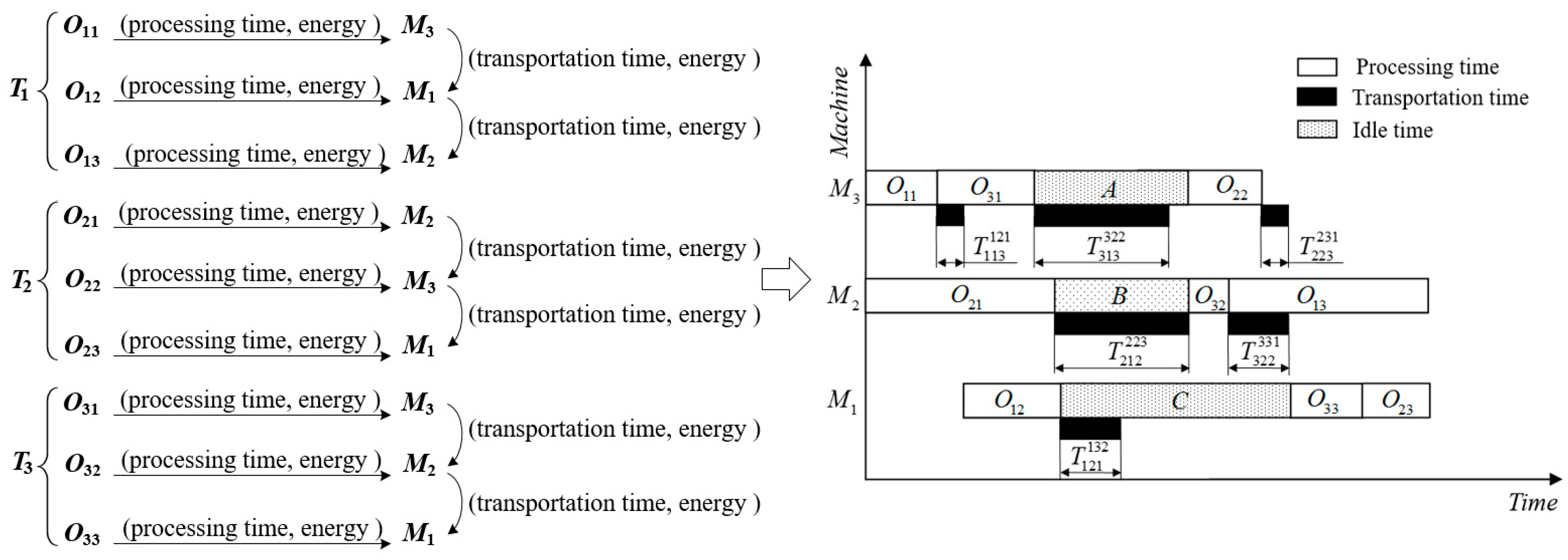
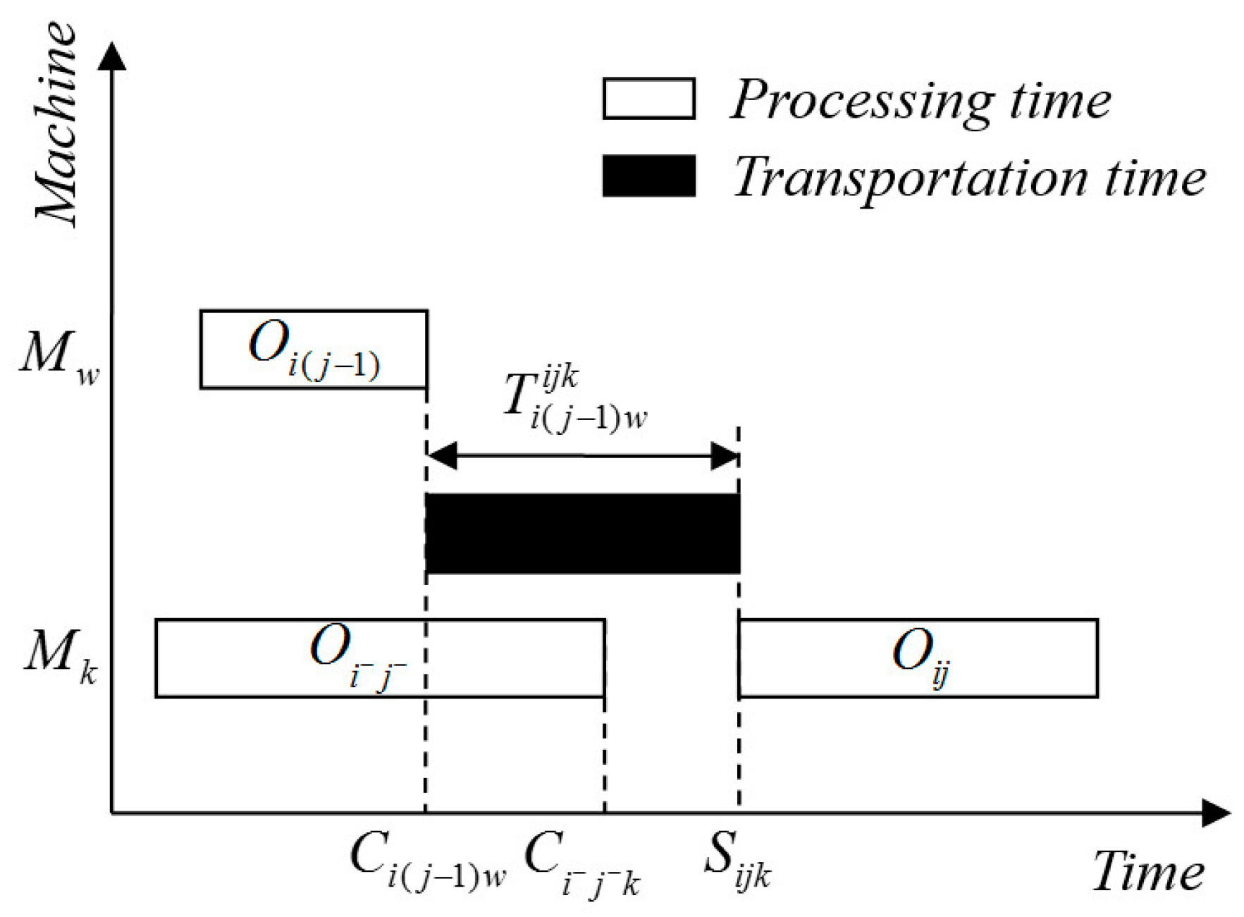
2.1. Problem Description

An energy-efficient job-shop scheduling problem with transportation constraints can be described as follows. There are a set of n tasks $T=\{T_1,T_2,\dots ,T_n\}$ and a set of m machines $M=\{M_1,M_2,\dots ,M_m\}$. Each task $T_i$ consists of a sequence of $N_i$ operations $(O_{i1},O_{i2},\dots ,O_{i{N}_i})$. All the operations must be executed by m machines in a fixed order. Once one operation $O_{ij}$ of a task $T_i$ completes its processing operation on a machine $M_w$, an empty AGV transfers the task to the next machine $M_w$ for processing. In the entire production process, both machines and AGVs consume energy for supporting production activities. The challenge is to determine the operation sequence on each machine to satisfy schedule efficiency that is measured in terms of makespan and energy efficiency that is calculated by the comprehensive energy required for a schedule. It is calculated by the comprehensive energy required for a schedule. For instance, as shown in Figure 1, there are three tasks and three machines. Each task has three operations, and the processing routings for them are M₃–M₁–M₂, M₂–M₃–M₁, and M₃–M₂–M₁, respectively. At the same time, the corresponding transportation times are collected. During the production process, each machine will consume energy to process each operation of the tasks, and AGVs will also consume energy to move the tasks. The objective of the EJSP is to find an effective and efficient schedule that minimizes the makespan and energy consumption. The EJSP satisfies the following assumptions.

(1)

Each task is available at time zero.

(2)

Each machine is available at time zero.

(3)

The precedence relationships between operations for each task cannot be changed.

(4)

Each machine can only process an operation of one task at a time.

(5)

Once an operation begins, the operation cannot be interrupted until it is completed.

(6)

There are enough AGVs responsible to move each task.

(7)

Handling times of all tasks between machines and AGVs are ignored.

2.2. Enhanced Estimation of Distribution Algorithm (EEDA)

Due to the strongly NP-hard nature of the job-shop scheduling problem (JSP), many optimization approaches such as meta-heuristic algorithms have been developed to obtain optimal and suboptimal solutions. It should be noted that although meta-heuristic approaches have been shown to be effective in solving the JSP with the consideration of energy efficiency [17,18,30], the solution quality will become less satisfactory, especially when transportation constraints are added to the scheduling model. The estimation of distribution algorithm (EDA), as an evolutionary algorithm, has received increasing interest in solving many complex optimization problems such as production scheduling problems [31,32,33].

In this section, an enhanced hybrid algorithm based on a combination of estimation of the distribution algorithm (EDA) and simulated annealing algorithm (SAA) is developed for solving the problem. In the literature, a variety of meta-heuristic algorithms have been used to solve JSP, including the genetic algorithm (GA), simulated annealing algorithm (SAA), estimation of distribution algorithm (EDA), particle swam optimization (PSO), etc. Among these algorithms, the EDA has the ability of global exploration and can quickly approach the optimization solution, but a fatal shortcoming is that its local exploitation ability is limited. Fortunately, SAA has a strong exploitation ability and can jump out of the local optimization to search for the best solution. Therefore, this paper proposes to incorporate the advantages of the SAA into the EDA. The EDA based on global information search is developed to rapidly obtain optimal or near-optimal solutions in the solution space, and then the SAA based on local information search is employed to seek better ones in terms of the solutions.

2.2.1. Representation

In this section, an encoding scheme based an operation representation is employed to study the EJSP with n tasks and m machines. For the EJSP, its encoding sequence consists of a series of tasks’ numbers and its encoding length (l) equals n × m. In the encoding sequence, different appearances of the same task number denote different operations of the task, and the j^th appearance represents the j^th operation of the task.

Example 1: Consider that the tasks are to be processed on three machines and each task has three operations, as shown in Figure 1. An encoding sequence (1 3 2 2 3 1 1 3 2) is yielded randomly. Here, 1, 2, and 3 represent the task number of T₁, T₂, and T₃, respectively. Moreover, take task T₁ for an example, there are three different appearances (i.e., the 1st, 6th, and 7th position) in the sequence, which means T₁ has three operations. The 1st position of the encoding sequence represents the first operation (O₁₁) of T₁; the 6th position of the encoding sequence represents the second operation (O₁₂) of T₁; the 7th position of the encoding sequence represents the third operation (O₁₃) of T₁. Thus, the corresponding operation sequence of the encoding sequence is (O₁₁, O₃₁, O₂₁, O₂₂, O₃₂, O₁₂, O₁₃, O₃₃, O₂₃).

Since the continuous space based on the EDA cannot be directly used to describe the discrete solution space of the EJSP, the sequence mapping method was developed in this paper. Firstly, generate random numbers ranging from 0 to 1 according to the encoding length; secondly, sort the numbers from small to large and record their corresponding position index; finally, divide each number by the total number of machines, and then round up to an integer.

Example 2: According to the encoding length in Figure 1, nine random numbers are generated as (0.104, 0.517, 0.618, 0.336, 0.988, 0.203, 0.380, 0.902, 0.151); then, the position indexes of the random numbers that are sorted from small to large are sequenced as (1, 9, 6, 4, 7, 2, 3, 8, 5); next, each number in the integer sequence is divided by three to acquire a value and the value is rounded up to an integer. Thus, the mapping result is (1, 3, 2, 2, 3, 1, 1, 3, 2).

2.2.2. Estimation of Distribution Algorithm

The estimation of distribution algorithm (EDA) is a global searching technique that is based on the probabilistic model [34]. Algorithm 1 shows the general steps of the EDA. In the EDA, the probabilistic model and updating mechanism are two crucial parts aspects.

Algorithm 1. Estimation of distribution algorithm (EDA)

Begin

Randomly generate the initial population X(0)

Set t = 0

While (the termination condition is not met) do

Select a set of candidate individuals (solutions) D(t) to construct the current population X(t) according to the fitness values

Construct the probability distribution model of the selected set D(t)

Generate a set of new offspring individuals N(t) according to the probabilistic model

Create a new population X(t + 1) by replacing some individuals of X(t) by N(t) according to the updating mechanism

T = t + 1

End while

Report best results

End

(1) Probabilistic model

The probabilistic model aims to reveal a general distribution by capturing the features of parent individuals. Moreover, the EDA generates new offspring individuals by sampling from the probabilistic model. Hence, constructing an effective probabilistic model is critical to studying the performance of the EDA. In this paper, according to the processing priorities of tasks, the probabilistic model was developed as an operation probabilistic matrix Q(t) with n rows and l columns.

$$Q(t)=\left[\begin{array}{cccc}{p}_{11}(t)& p_{12}(t)& \cdots & p_{1l}(t)\\ p_{21}(t)& p_{22}(t)& \cdots & p_{2l}(t)\\ ⋮& ⋮& \ddots & ⋮\\ p_{n1}(t)& p_{n2}(t)& \cdots & p_{nl}(t)\end{array}\right]$$

(1)

where $p_{iq}(t)(1\le i\le n,1\le l\le n\times m)$ stands for an element of the operation probabilistic matrix Q(k), which represents the probability that task T_i appears in the q^th position of the operation sequence vector at generation t. Here, there exists $p_{iq}(t)\in [0,1]$ and ${\displaystyle {\sum }_{i=1}^n{p}_{iq}(t)=1},(\forall q)$ at generation t. At the initial stage of the proposed algorithm, the value of each element in Q(t) is initialized as $p_{iq}(0)=1/n,(\forall i,q)$.

(2) Updating mechanism

In order to enhance the exploitation ability of the EDA, the probabilistic model should be adjusted well at each generation. Hence, an updating mechanism based on the incremental learning method was developed in this paper. First, according to the roulette wheel selection strategy, a promising sub-population that consists of Num_SP candidate solutions was determined. Then, the operation probabilistic matrix Q(t) was updated based on the information of the promising sub-population and the historical information. The updating function of the probabilistic model is formally defined as:

$$p_{iq}(t+1)=(1-\alpha )·p_{iq}(t)+\frac{\alpha }{Num\_SP}{\displaystyle \sum _{s=1}^{Num\_SP}{\delta }_{iq}^s},\forall i,q$$

(2)

where $\alpha$ represents the learning rate of the operation probabilistic matrix Q(t), and $\alpha \in (0,1)$; ${\delta }_{iq}^s$ represents the following indicator function of the s^th candidate individual in the promising sub-population.

$${\delta }_{{}_{iq}}^s=\{\begin{array}{l}1,\mathrm{if}\mathrm{task}{T}_i\mathrm{appears}\mathrm{in}\mathrm{the}{q}^{\mathrm{th}}\mathrm{position}\\ 0,\mathrm{else}\end{array}$$

(3)

2.2.3. Simulated Annealing Algorithm

The simulated annealing algorithm (SAA) is a stochastic searching technique and its local search ability is promising. Algorithm 2 shows the general steps of the SAA. In the SAA, the neighborhood structure and annealing rate function have an important impact on performance.

Algorithm 2. Simulated annealing algorithm (SAA)

Begin

Generate the initial schedule Si

Initialize the start temperature Ts, the end temperature Te

Set T = Ts

While (T > Te) do

Generate the temporary schedule Sj according to the neighborhood structure

Evaluate the improvement of performance criterion function Δ = f(Sj) − f(Si)

If (Δ ≤ 0) then

Si = Sj

Else if (random(0,1) < e−Δ/T) then

Si = Sj

End if

Update new annealing rate function

End while

Report best results

End

(3) Neighborhood structure

To create a set of feasible solutions, neighborhood structures are needed. In general, the disjunctive graph is used to describe the neighborhood structure. In the neighborhood structures, the neighborhoods are generated in terms of neighborhood strategies. One of the most effective neighborhood strategies is based on the block structure of the critical path method, which is adapted in the SAA. A critical path, which is the longest path in the disjunctive graph, consists of a series of operations. It corresponds to a feasible solution. A maximal sequence of several operations that either is processed on the same machine or belongs to the same task is defined as a critical block. In this paper, the swap neighborhood structure based on the critical block is presented to generate the neighborhood.

(4) Annealing rate function

Annealing rate directly affects the speed and accuracy of the SAA. The general annealing rate function is given by Equation (4).

$$T(t)=\beta \times T(t-1)$$

(4)

where $\beta \in (0,1)$ represents an annealing rate coefficient; T(t) and T(t − 1) represent current temperature and previous temperature, respectively; t represents the iteration number.

According to the characteristic of the annealing temperature function, it can be obtained that its decreased amplitude becomes faster at a high temperature level, while its decreased amplitude becomes slower at a low temperature level. It is likely to result in an insufficient search in the solution space. In order to enhance the exploitation ability of the SAA, an improved annealing rate function inspired by the Hill function is developed as

$$T(t)=\beta \times \frac{T_0{}^n}{T_0{}^n+t^n}$$

(5)

where T₀ represents a temperature threshold and it has a relationship with an initial temperature of the SAA; n represents a Hill coefficient, and $n\ge 1$; $\beta \in (0,1)$ represents an annealing rate coefficient; t represents the iteration number.

2.2.4. The Procedure of the EEDA

By embedding SAA into EDA, an enhanced estimation of distribution algorithm (EEDA) was developed to solve the EJSP. To balance the global exploration and local exploitation of the EEDA, a decision-making factor $\lambda$ was designed with Equation (6). The procedure of the EEDA is described as shown in Algorithm 3.

$$\lambda (t)=\exp (-t/Maxgen)$$

(6)

where t represents the iteration number; Maxgen represents the maximal number of iteration.

Algorithm 3. Enhanced Estimation of distribution algorithm (EEDA)

Begin

Randomly generate the initial population X(0)

Initialize the learning rate α, the Hill coefficient n, the start temperature Ts, the end temperature Te

Set t = 0, T = Ts

While (the termination condition is not met) do

Evaluate the fitness value of each individual in X(0)

Select a set of candidate individuals (solutions) D(t) to construct the current population X(t)

Construct the probability distribution model of the selected set D(t)

If (rand ≤ λ) then

Generate a set of new offspring individuals N(t) according to the probabilistic model

Create a new population X(t + 1) by replacing some individuals of X(t) by N(t) according to the updating mechanism

Else

While (T >Te) do

Generate the temporary individuals N(t) according to the neighborhood structure

Evaluate the improvement of the fitness value

Update annealing rate function

End while

End if

T = t + 1

End while

Report best results

End

3. Model of Energy-Efficient Job-Shop Scheduling Problem (EJSP) with Transportation Constraints

3.1. Notations

Notations are defined as follows.

i, i−	Index of tasks
j, j−	Index of operations
k, w	Index of machines
q	Index of position
n	Number of tasks
m	Number of machines
T	Set of tasks, T = {T1, T2, …, Tn}
M	Set of machines, M = {M1, M2, …, Mm}
Oij	jth operation of task Ti
Ni	Number of operations for task Ti
Qk	Number of operations processed on machine Mk
Ci	Completion time of task Ti
Cmax	Completion time of the last task
Bkq	Starting time of the operation allocated to the qth position on machine Mk
Sijk	Starting time of operation Oij on machine Mk
Cijk	Completion time of operation Oij on machine Mk
Ci−j−k	Completion time of the preceding operation of operation Oij on machine Mk
Tijk	Processing time of operation Oij on machine Mk
$T_{i(j-1)w}^{ijk}$	Transportation time needed to move from machine Mw to machine Mk for two successive operations Oi(j−1) and Oij of task Ti
Pijk	Processing power of operation Oij on machine Mk
Pk	Unload power of machine Mk
P0	Transportation power of automatic guided vehicle
E	Comprehensive energy consumption for a schedule
Ec	Energy consumption module for cutting process
Ei	Energy consumption module for idle running process
Et	Energy consumption module for transportation process
Ea	Energy consumption module for auxiliary process
e	Average energy requirement per unit time for auxiliary equipment
L	A big positive number
Yijkq	Sequencing binary variable that is set to 1 if operation Oij is to be processed in qth position on machine Mk, and 0 otherwise

3.2. Energy Consumption Model

According to energy-consuming behaviors of each task processed on machines [15,16], three important energy consumption modules were considered: energy consumption module for a cutting process (Ec), energy consumption module for an idle running process (Ei), and energy consumption module for an auxiliary process (Ea). In addition, AGVs are used to move each task that needs to be transported to the next machine after the completion of a task on a machine, which also consumes energy, i.e., energy consumption module for a transportation process (Et). Thus, the comprehensive energy consumption throughout the production process mainly consists of four modules, which are described as follows.

3.2.1. Energy Consumption Module for a Cutting Process (Ec)

Ec represents the energy required to execute all the operations. In general, Ec can be calculated approximately by using a secondary polynomial fitting curve [35]. Hence, the formulation of Ec is defined below.

$$Ec={\displaystyle \sum _{k=1}^m{P}_k·}({\displaystyle \sum _{i=1}^n{\displaystyle \sum _{j=1}^{N_i}{T}_{ijk}}})+{\displaystyle \sum _{i=1}^n{\displaystyle \sum _{j=1}^{N_i}{\displaystyle \sum _{k=1}^m(1+{\alpha }_1)·P_{ijk}·}}}{T}_{ijk}+{\displaystyle \sum _{i=1}^n{\displaystyle \sum _{j=1}^{N_i}{\displaystyle \sum _{k=1}^m{\alpha }_2·P_{ijk}{}^2·}}}{T}_{ijk}$$

(7)

where ${\alpha }_1$ and ${\alpha }_2$ are the coefficients of the secondary polynomial fitting curve.

3.2.2. Energy Consumption Module for an Idle Running Process (Ei)

Ei represents the energy required to wait for processing the next operation when a machine is in an idle running period. Ei can be calculated by multiplying the unload power consumption by the total idle time as:

$$Ei={\displaystyle \sum _{k=1}^m{P}_k}·(\underset{i,j}{\max }{C}_{ijk}-{\displaystyle \sum _{i=1}^n{\displaystyle \sum _{j=1}^{N_i}(C_{ijk}-S_{ijk})}})$$

(8)

3.2.3. Energy Consumption Module for an Auxiliary Process (Ea)

Ea represents the energy required to support production equipment in the workshop, such as lighting, heating, and air-conditioning. Ea can be written as:

$$Ea=e·\underset{1\le i\le n}{\max }(C_i)$$

(9)

3.2.4. Energy Consumption Module for a Transportation Process (Et)

Et is the energy consumption of an AGV for moving a task whenever it requires transportation from one machine to another. Et is defined as:

$$Et={\displaystyle \sum _{i=1}^n{\displaystyle \sum _{j=2}^{N_i}{\displaystyle \sum _{k=1}^m{\displaystyle \sum _{w=1}^m{P}_0·T_{i(j-1)w}^{ijk}}}}}$$

(10)

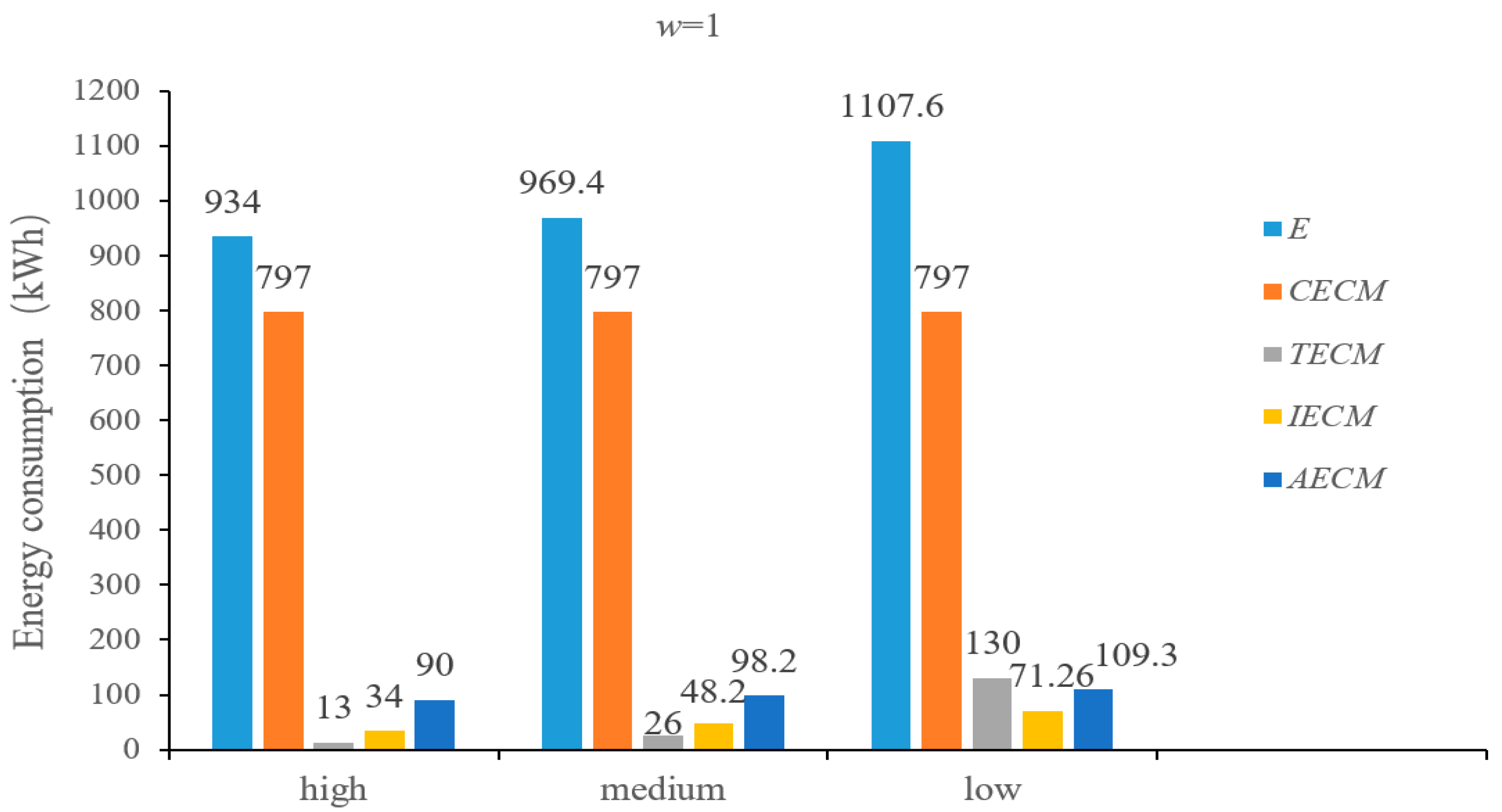
3.2.5. Comprehensive Energy Consumption (E)

E is composed of Ec, Ei, Ea, and Et. Hence, the comprehensive energy consumption is the sum of them, which is expressed as:

$$E=Ec+Ei+Ea+Et$$

(11)

3.3. Formulation of the EJSP Optimization Model

The scheduling optimization objectives are to satisfy two efficiency criteria: schedule efficiency that is measured in terms of makespan and energy efficiency that is calculated by the comprehensive energy consumption for a schedule. The two objective functions can be written as:

$$\min f_1=C_{\max }$$

(12)

$$\min f_2=E$$

(13)

subject to:

$$\begin{array}{l}{C}_{ijk}-C_{i(j-1)w}\ge T_{ijk};\\ \forall i=1,2,\dots ,n,j=2,3,\dots ,N_i,k,w=1,2,\dots ,m\end{array}$$

(14)

$$\begin{array}{l}{S}_{ijk}\ge \max (C_{i(j-1)w}++T_{i(j-1)w}^{ijk},C_{i^{-}{j}^{-}k})\\ \forall i,i^{-}=1,2,\dots ,n,j=2,3,\dots ,N_i,j^{-}=1,2,\dots ,N_{i^{-}},k,w=1,2,\dots ,m\end{array}$$

(15)

$$\begin{array}{l}{B}_{kq}\le T_{ijk}+L·(1-Y_{ijkq});\\ \forall i=1,2,\dots ,n,j=1,2,\dots ,N_i,k=1,2,\dots ,m,q=1,2,\dots ,Q_k;\end{array}$$

(16)

$$\begin{array}{l}{B}_{kq}\ge T_{ijk}-L·(1-Y_{ijkq});\\ \forall i=1,2,\dots ,n,j=1,2,\dots ,N_i,k=1,2,\dots ,m,q=1,2,\dots ,Q_k;\end{array}$$

(17)

$$\begin{array}{l}{\displaystyle \sum _{i=1}^n{\displaystyle \sum _{j=1}^{N_i}{Y}_{ijkq}=1}};\\ \forall k=1,2,\dots ,m,q=1,2,\dots ,Q_k\end{array}$$

(18)

The first objective (12) is to minimize the makespan and the second objective (13) is to minimize the comprehensive energy consumption. Constraint (14) ensures that the precedence constraints between the operations of each task are not changed. Constraint (15) establishes the relationship between the transportation constraint and the machine capacity constraint. Assume that two adjacent operations (O_i⁻j⁻, O_ij) are to be executed on machine M_k in Figure 2. The completion time of the preceding operation O_i⁻j⁻ of operation O_ij on machine M_k is C_i⁻j⁻k, the completion time of the (j − 1)^th operation O_i(j−1) of task T_i on machine M_w is C_i(j−1)w, and the transportation time of AGV between machine M_w and machine M_k is $T_{i(j-1)w}^{ijk}$. If $C_{i^{-}{j}^{-}k}\le C_{i(j-1)w}+T_{i(j-1)w}^{ijk}$, then, the start time of operation O_ij should be after the transportation time of operation O_i(j−1). Otherwise, the start time of operation O_ij should be after the completion time of operation O_i⁻j⁻. Constraints (16) and (17) establish linking constraints between start times B_kq and S_ijk. It means that if operation O_ij is processed in the q^th position on machine M_k, then B_kq = S_ijk. Constraint (18) points out that an operation is only assigned to one position of one machine.

As the relationship between energy consumption and makespan is conflicting, no single optimal solution exists in the multi-objective optimization problem (MOP) [36]. There have been diverse techniques for solving MOP. One of the most popular approaches to studying MOP is the normalized weighted additive utility function (NWAUF). Owning to its simplicity and natural ability to explore efficient solutions, the NWAUF has been successfully applied in the field of production scheduling. The NWAUF for alternative k with n objectives is defined as U(k):

$$U(k)=w_1{f^{\prime }}_1(k)+w_2{f^{\prime }}_2(k)+\dots +w_n{f^{\prime }}_n(k)$$

(19)

where w_i(i = 1, 2, …, n) is a weight coefficient, and ${\displaystyle \sum _{i=1}^n{w}_i}=1$, $w_i\in [0,1]$; $f_i{}^{\prime }(k)$ is the normalized value of the i^th objective function $f_i(k)$ for $i=1,2,\dots ,n$. Note that each normalized objective $f_i{}^{\prime }(k)$ can be expressed by Equation (20).

$$f_i{}^{\prime }(k)=\frac{f_{i,\max }-f_i(k)}{f_{i,\max }-f_{i,\min }}$$

(20)

where $f_{i,\min }$ and $f_{i,\max }$ represent for the minimum and maximum values of the objective function $f_i$, respectively.

Using the utility function, MOP can be solved as a single objective optimization. Therefore, according to the objective functions (12) and (13), NWAUF is formulated as F(k):

$$F(k)=w·\frac{f_{1,\max }-f_1(k)}{f_{1,\max }-f_{1,\min }}+(1-w)·\frac{f_{2,\max }-f_2(k)}{f_{2,\max }-f_{2,\min }}$$

(21)

where $w$ is the weighted importance of the objective function makespan and $w\in [0,1]$. $f_{1,\min }$ and $f_{1,\max }$ are the minimum and maximum values of the objective function $f_1$, respectively. $f_{2,\min }$ and $f_{2,\max }$ are the minimum and maximum values of the objective function $f_2$, respectively.

4. Experimental Results

In this section, the proposed EEDA is employed to solve the EJSP. First, the analysis of the algorithm parameter settings was conducted to investigate their influence on the performance of the EEDA. Second, two classes of benchmark instances from the OR-Library were given to evaluate the performance of the proposed algorithm. Finally, the proposed algorithm was used to evaluate the effectiveness of the proposed model. The computational experiments were carried out utilizing MATLAB R2009a. The experimental tests were implemented on a personal computer with an Intel Pentium (R) with 4 GB memory and a 2.60 GHz processor, and the operating system was Windows 10.

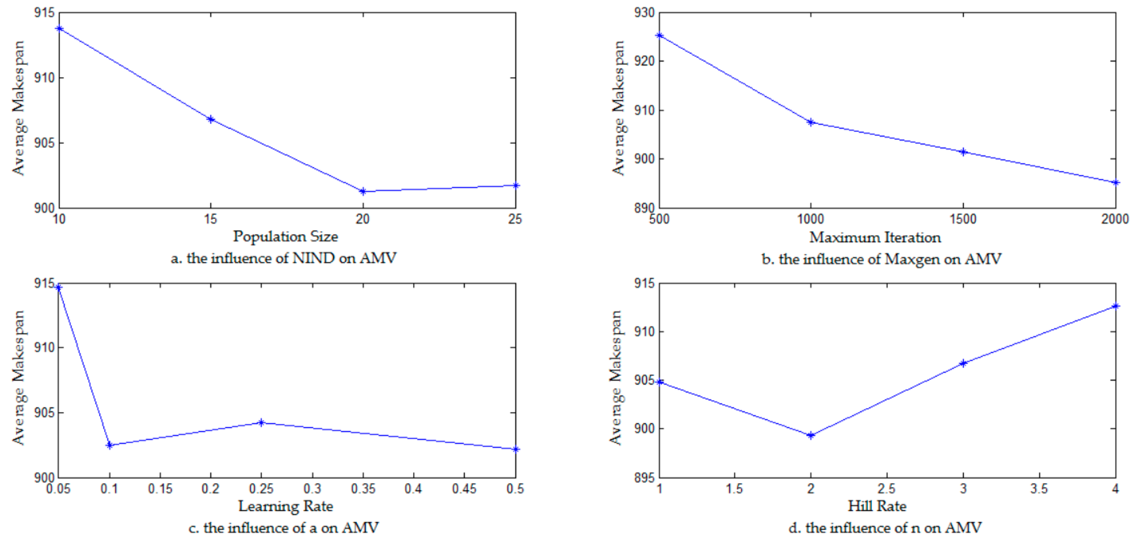
4.1. Sensitivity Analysis of the Algorithm Parameters

The parameter settings could have significant influence on the performance of the EEDA. In the EEDA, four critical algorithm parameters should be considered: the population size (NIND), the maximum number of iterations (Maxgen), the learning rate ($\alpha$), and the Hill coefficient (n). In order to analyze the influence of these algorithm parameters on the performance of the EEDA, the Taguchi design method was adopted to study the parametric sensitivity. An example of a 10 × 10 JSP is given in

Table 1. Test instance with 10 tasks 10 machines.

	Operations	(Machine Number, Processing Time/min)
Tasks		1	2	3	4	5	6	7	8	9	10
T1		(3,29)	(10,43)	(2,85)	(1,71)	(4,6)	(8,47)	(6,37)	(5,86)	(7,76)	(9,13)
T2		(2,78)	(7,28)	(3,51)	(6,81)	(5,22)	(10,2)	(1,16)	(4,46)	(9,69)	(8,85)
T3		(10,9)	(3,90)	(7,74)	(4,95)	(6,14)	(1,84)	(8,13)	(2,31)	(5,85)	(9,61)
T4		(2,36)	(1,69)	(10,39)	(3,8)	(7,26)	(4,85)	(9,61)	(5,19)	(6,76)	(8,52)
T5		(3,49)	(7,75)	(2,33)	(5,99)	(8,69)	(9,6)	(6,35)	(1,32)	(4,26)	(10,90)
T6		(9,11)	(7,46)	(2,10)	(8,43)	(4,11)	(6,52)	(10,21)	(1,74)	(5,11)	(3,47)
T7		(1,62)	(2,46)	(10,89)	(7,19)	(3,13)	(4,65)	(9,32)	(5,88)	(6,40)	(8,7)
T8		(7,56)	(2,72)	(3,12)	(6,25)	(10,49)	(5,25)	(1,30)	(4,36)	(9,79)	(8,45)
T9		(10,44)	(3,30)	(4,90)	(7,52)	(1,21)	(8,48)	(6,89)	(2,19)	(5,74)	(9,64)
T10		(1,21)	(9,11)	(7,45)	(4,22)	(6,72)	(10,72)	(8,32)	(2,48)	(5,11)	(3,76)

. There are 10 types of tasks to be processed on 10 machines, and each task contains 10 operations. An operation is assigned to a given machine and has the corresponding processing time. For example, in Table 1, the element (4,6) in first row and fifth column means that the 5th operation of task T₁ is processed on machine M₄ and the processing time is 6 min. Here, for the convenience of analysis and comparison, the scheduling objective is to minimize the makespan which is used by many authors in the literature. Various values for the four parameters are listed

Table 2. Various values of the algorithm parameters.

Variables	Value
	1	2	3	4
NIND	10	15	20	25
Maxgen	500	1000	1500	2000
α	0.05	0.1	0.25	0.5
n	1	2	3	4

. In addition, the average makespan value (AMV) and average running time (ART) were adopted as evaluation standards to analyze the parameters.

The experimental results on the combination situations of the four parameters are listed

Table 3. Combination situations of the algorithm parameters.

Number	NIND	Maxgen	α	n	AMV	ART(s)
1	1	1	1	1	946.4	84.76
2	1	2	2	2	903.8	169.55
3	1	3	3	3	902.6	255.75
4	1	4	4	4	902.2	339.42
5	2	1	2	3	925.4	130.50
6	2	2	1	4	918.2	262.10
7	2	3	4	1	895.8	434.90
8	2	4	3	2	887.8	515.95
9	3	1	3	4	924	178.05
10	3	2	4	3	905.8	344.34
11	3	3	1	2	900.8	503.77
12	3	4	2	1	874.4	734.28
13	4	1	4	2	905	238.63
14	4	2	3	1	902.4	474.98
15	4	3	2	4	906.2	642.57
16	4	4	1	3	893.2	840.01

. Figure 3 describes the changing trend in the average makespan, such that each parameter for different setting values is considered.

From Table 3 and Figure 3, it can be seen that four parameters had an impact on the performance of the EEDA. Concretely speaking, the average makespan value decreased as any of these parameter values (including NIND, Maxgen, $\alpha$) increased, as shown in Figure 3a–c. But a large parameter setting value could result in more computational time. In addition, when the Hill coefficient was set to 2, in Figure 3d, the better solution can be obtained by the EEDA. Therefore, according to the above analysis, the parameter values in the EEDA are set in Table 2 (in bold and italics).

4.2. Performance Evaluation

To validate the effectiveness of the proposed algorithm, the widely used benchmark instances from the OR-library were carried out [37]. Two classes of benchmarks instances are considered: one was the instance FT06, FT10, FT20 (n × m = 6 × 6, 10 × 10, 20 × 5) designed by Fisher and Thompson [38], the other was the instance LA01-LA40 (n × m = 10 × 5, 15 × 5, 20 × 5, 10 × 10, 15 × 10, 20 × 10, 30 × 10, 15 × 15) designed by Lawrence [39]. The proposed algorithm was compared with several existing algorithms, including estimation of distribution algorithm (EDA) presented by He et al. [40], hybrid differential evolution and estimation of distribution algorithm (DE-EDA) presented by Zhao et al. [41], simulated annealing (SA) presented by Laarhoven et al. [42], hybrid genetic and simulated annealing (GA–SA) presented by Wang and Zheng [43], genetic algorithm (GA: P-GA, SBGA-40, SBGA-60 ) presented by Dorndorf and Pesch [44], and hybrid genetic algorithm (HGA: HGA-Param, HGA-Non-delay, HGA-Active) presented by Goncalves et al. [45]. For each instance, we ran the algorithms 10 times independently. The experimental results are shown in

Table 4. Experimental results obtained by different algorithms.

Instance	Size	Sbest	EEDA	EDA [40]	EDA- DE [41]	SA [42]	GA-SA [43]	GA [44]			HGA [45]
								P-GA	SBGA- 40	SBGA- 60	HGA- Param	HGA-Non-delay	HGA- Active
FT06	6 × 6	55	55	55	55	55	55	-	-	-	55	55	55
FT10	10 × 10	930	930	937	937	930	930	960	-	-	930	951	945
FT20	20 × 5	1165	1165	1184	1178	1165	1165	1249	-	-	1165	1178	1173
LA01	10 × 5	666	666	666	666	666	666	666	666	-	666	666	666
LA02	10 × 5	655	655	-	655	655	-	681	666	-	655	665	655
LA03	10 × 5	597	597	-	597	606	-	620	604	-	597	604	603
LA04	10 × 5	590	590	-	590	590	-	620	590	-	590	590	598
LA05	10 × 5	593	593	-	593	593	-	593	593	-	593	593	593
LA06	15 × 5	926	926	926	926	926	926	926	926	-	926	926	926
LA07	15 × 5	890	890	-	890	890	-	890	890	-	890	890	890
LA08	15 × 5	863	863	-	863	863	-	863	863	-	863	863	863
LA09	15 × 5	951	951	-	951	951	-	951	951	-	951	951	951
LA10	15 × 5	958	985	-	958	958	-	958	958	-	958	958	958
LA11	20 × 5	1222	1222	1222	1222	1222	1222	1222	1222	-	1222	1222	1222
LA12	20 × 5	1039	1039	-	1039	1039	-	1039	1039	-	1039	1039	1039
LA13	20 × 5	1150	1150	-	1150	1150	-	1150	1150	-	1150	1150	1150
LA14	20 × 5	1292	1292	-	1292	1292	-	1292	1292	-	1292	1292	1292
LA15	20 × 5	1207	1207	-	1207	1207	-	1237	1207	-	1207	1207	1207
LA16	10 × 10	945	945	945	956	956	945	1008	961	961	945	973	947
LA17	10 × 10	784	784	-	784	784	-	809	787	784	784	792	784
LA18	10 × 10	848	859	-	855	861	-	916	848	848	848	855	848
LA19	10 × 10	842	842	-	852	848	-	880	863	848	842	851	852
LA20	10 × 10	902	902	-	907	902	-	928	911	910	907	926	912
LA21	15 × 10	1046	1060	1071	1058	1063	1058	1139	1074	1074	1046	1079	1074
LA22	15 × 10	927	938	-	952	938	-	998	935	936	935	950	962
LA23	15 × 10	1032	1032	-	1038	1032	-	1072	1032	1032	1032	1032	1032
LA24	15 × 10	935	948	-	973	952	-	1014	960	957	953	970	955
LA25	15 × 10	977	989	-	1000	992	-	1014	1008	1007	986	1013	1014
LA26	20 × 10	1218	1218	1257	1229	1218	1218	1278	1219	1218	1218	1218	1237
LA27	20 × 10	1235	1270	-	1287	1269	-	1378	1272	1269	1256	1282	1280
LA28	20 × 10	1216	1218	-	1275	1224	-	1327	1240	1241	1232	1250	1250
LA29	20 × 10	1152	1200	-	1220	1203	-	1336	1204	1210	1196	1206	1226
LA30	20 × 10	1355	1355	-	1371	1355	-	1411	1355	1355	1355	1355	1355
LA31	30 × 10	1784	1784	1789	1784	1784	1784	-	-	-	1784	1784	1784
LA32	30 × 10	1850	1850	-	1850	1850	-	-	-	-	1850	1850	1850
LA33	30 × 10	1719	1719	-	1719	1719	-	-	-	-	1719	1719	1719
LA34	30 × 10	1721	1721	-	1721	1721	-	-	-	-	1721	1721	1721
LA35	30 × 10	1888	1888	-	1888	1888	-	-	-	-	1888	1888	1888
LA36	15 × 15	1268	1290	1292	1315	1293	1292	1373	1317	1317	1279	1303	1313
LA37	15 × 15	1397	1445	-	1465	1433	-	1498	1484	1446	1408	1437	1444
LA38	15 × 15	1196	1210	-	1244	1215	-	1296	1251	1241	1219	1252	1228
LA39	15 × 15	1233	1255	-	1291	1248	-	1351	1282	1277	1246	1250	1265
LA40	15 × 15	1222	1236	-	1277	1234	-	1321	1274	1252	1241	1252	1246

“-” means inapplicable.

. It lists the problem name, the problem size, the best-known solution (S_best), the solution obtained by the proposed algorithm (EEDA), and the solution obtained by other algorithms reported in the literature. According to Table 4, it can be observed that the proposed algorithm obtained the best-known solution in 30 out of 43 instances. In other words, the EEDA found the best-known solution in 70% of problem instances. In addition, compared with EDA and SA, the EEDA was superior to them in solution quality. Hence, the combination of the EDA and SA is promising in solving the problems.

At the same time, average relative percentage deviation (ARPD) is designed to evaluate the performance of the EEDA in the experimental test as below:

$$ARPD=({\displaystyle \sum _{z=1}^{\mathrm{NIS}}\frac{f(z)-S_{best}}{S_{best}}\times 100})/\mathrm{NIS}$$

(22)

where f(z) represents the best result obtained by the algorithms, S_best represents the best result known for each instance, NIS represents the number of instances solved by the algorithms.

In addition, improvement rate (IR) of ARPD obtained by the EEDA with regard to other algorithms is defined as follows:

$$IR=\frac{ARPD\mathrm{of}\mathrm{some}\mathrm{algorithm}-ARPD\mathrm{of}\mathrm{EEDA}}{ARPD\mathrm{of}\mathrm{some}\mathrm{algorithm}}$$

(23)

The comparisons of the experimental results among different algorithms are given in

Table 5. Experimental results of the EEDA compared with the other algorithms.

Algorithms	NIS	ARPD		IR
		Others	EEDA
EDA [40]	11	0.92	0.28	0.70
EDA-DE [41]	43	0.80	0.60	0.25
SA [42]	43	0.63	0.60	0.05
GA-SA [43]	11	0.28	0.28	0
P-GA [44]	37	4.62	0.69	0.85
SBGA-40 [44]	35	1.43	0.73	0.49
SBGA-60 [44]	20	1.97	1.14	0.42
HGA-Param [45]	43	0.40	0.60	-0.50
HGA-Non-delay [45]	43	1.23	0.60	0.51
HGA-Active [45]	43	1.12	0.60	0.46

. It lists the different algorithms, the number of instances solved (NIS), the average relative percentage deviation (ARPD) of all compared algorithms, and the corresponding improvement rate (IR). From Table 5, we can find that the ARRD of the EEDA was 0.60 in all 43 instances. Compared to the other algorithms, the EEDA had an improvement in solution quality.

In summary, it was realized that the proposed algorithm is a promising approach for the job shop scheduling problem by comparing it with other algorithms. Thus, the EEDA is employed to solve the EJSP in the next section.

4.3. Case Study

In order to evaluate the energy-savings potential of the proposed model, an experiment originating from a machining shop floor is illustrated: the experiment consists of ten tasks and ten machines. These tasks had similar processing operations, including rough/finish turning, rough/finish milling, drilling/tapping, rough/finish grinding, cleaning, and inspection. Their processing times are shown in

Table 6. Processing times of tasks on machines (unit: s).

	Operations	(Machine Number, Processing Time)
Tasks		1	2	3	4	5	6	7	8	9	10
T1		(1,1740)	(2,4680)	(3,600)	(4,2160)	(5,3000)	(6,660)	(7,3720)	(8,3360)	(9,2640)	(10,1260)
T2		(1,2580)	(3,5400)	(5,4500)	(10,660)	(4,4140)	(2,1680)	(7,2760)	(6,2760)	(8,4320)	(9,1800)
T3		(2,5460)	(1,5100)	(4,2340)	(3,4440)	(9,5400)	(6,600)	(8,720)	(7,5340)	(10,2700)	(5,2580)
T4		(2,4860)	(3,5700)	(1,4260)	(5,5940)	(7,540)	(9,3120)	(8,5100)	(4,5880)	(10,1320)	(6,2580)
T5		(3,840)	(1,360)	(2,1320)	(6,3660)	(4,1560)	(5,4140)	(9,1260)	(8,2940)	(10,4320)	(7,3180)
T6		(3,5040)	(2,120)	(6,3120)	(4,5700)	(9,2880)	(10,4320)	(1,2820)	(7,3900)	(5,360)	(8,1500)
T7		(2,2760)	(1,2220)	(4,3660)	(3,780)	(7,1920)	(6,1260)	(10,1920)	(9,5340)	(8,1800)	(5,3300)
T8		(3,1860)	(1,5160)	(2,2760)	(6,4440)	(5,1920)	(7,5280)	(9,1140)	(10,2880)	(8,2160)	(4,4740)
T9		(1,4560)	(2,4140)	(4,4560)	(6,3060)	(3,5100)	(10,660)	(7,2400)	(8,5340)	(5,1560)	(9,4440)
T10		(2,5100)	(2,780)	(3,3660)	(7,420)	(9,3840)	(10,4560)	(6,2820)	(4,3120)	(5,5400)	(8,2700)

. Moreover, there were five AGVs for transporting the tasks among machines, and the power demand of each AGV was set to 3.45 kW. In addition, the auxiliary average power required to support the production environment was set to 1 kW. The transportation times between different machines are listed in

Table 7. Transportation times between different machines (unit: s).

Machine Number	M1	M2	M3	M4	M5	M6	M7	M8	M9	M10
M1	0	152	170	193	100	112	173	165	142	133
M2	152	0	131	138	152	169	120	170	162	143
M3	170	131	0	160	151	140	132	171	122	140
M4	193	138	160	0	140	140	165	170	140	198
M5	100	152	151	140	0	103	102	170	180	192
M6	112	169	140	140	103	0	142	140	148	150
M7	173	120	132	165	102	142	0	150	162	160
M8	165	170	171	170	170	140	150	0	141	120
M9	142	162	122	140	180	148	162	141	0	153
M10	133	143	140	198	192	150	160	120	153	0

. The related power demand for all machines is given in

Table 8. Unload power of each machine.

Machine Number	M1	M2	M3	M4	M5	M6	M7	M8	M9	M10
Processing power (kW)	18	15	6	12	10	5.5	7.5	3	5.5	10
Unload power (kW)	2.4	3.36	2.0	1.77	2.2	2.55	2.02	1.77	1.16	1.8

.

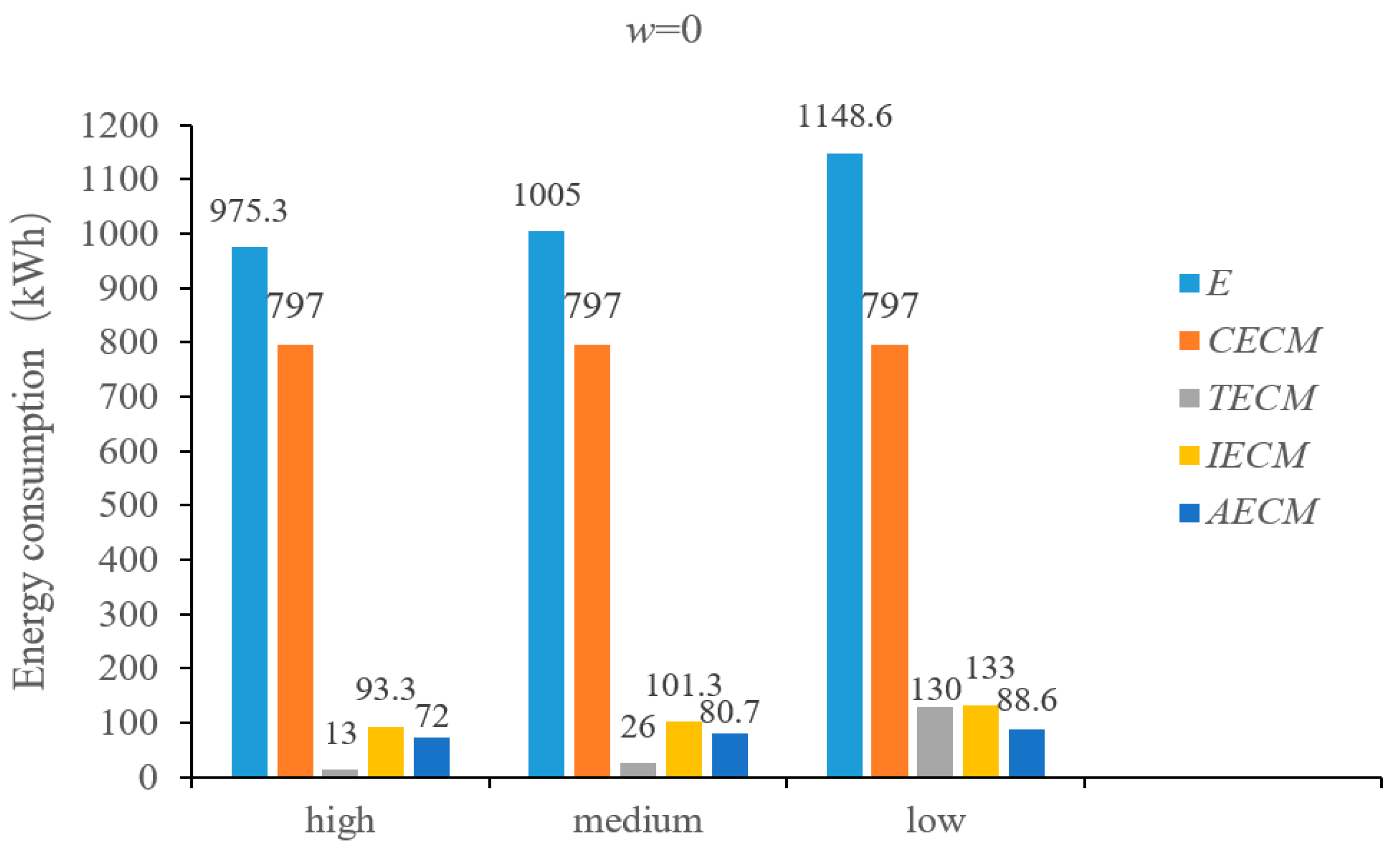
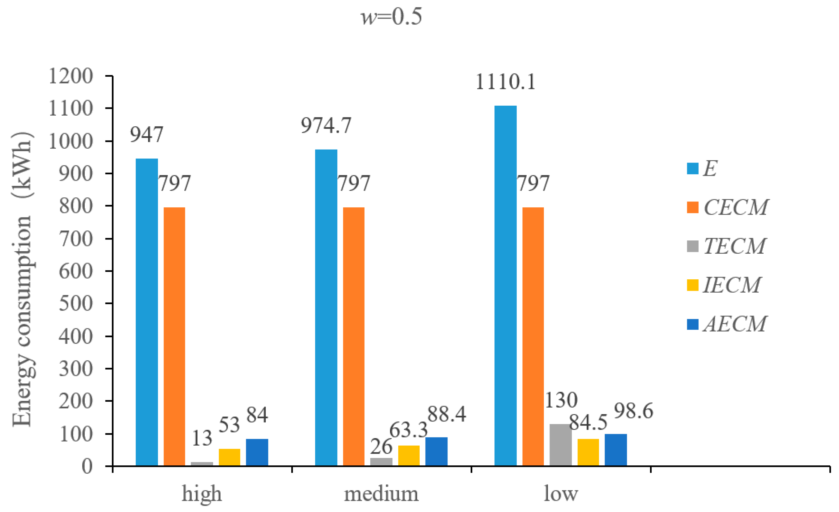
4.3.1. Energy-Efficient Scheduling Analysis

To highlight the transportation impact over the scheduling objective, we analyzed energy consumptions with regard to different transportation speeds of AGVs. Three transportation speeds, i.e., low speed, medium speed, and high speed, were considered when the weighted importance w was set as 0, 0.5, and 1, respectively. The experimental results based on the proposed EEDA are shown in Figure 4, Figure 5 and Figure 6.

From the results shown in Figure 4, Figure 5 and Figure 6, we can observe that the ratio of the transportation energy consumption to the comprehensive energy consumption became lower as the transportation speed increased for the given weighted importance. Moreover, the comprehensive energy consumption reduced as the transportation speed increased. It is also clear that the comprehensive energy consumption decreased as the weighted importance w increased at the given transportation speed. Furthermore, the transportation speed had a significant effect on Ei and Ea. For example, for the given weighted importance (w = 0.5), when the transportation speed increased from low speed to the high speed, the ratio of the idle energy consumption decreased to 36.9% and the ratio of the auxiliary energy consumption decreased to 14.29%. Also, we calculated that the comprehensive energy consumption ratio decreased to 14.61%. Therefore, it was concluded that the energy-efficient scheduling strategy could be considered by increasing the transportation speed for the decision makers.

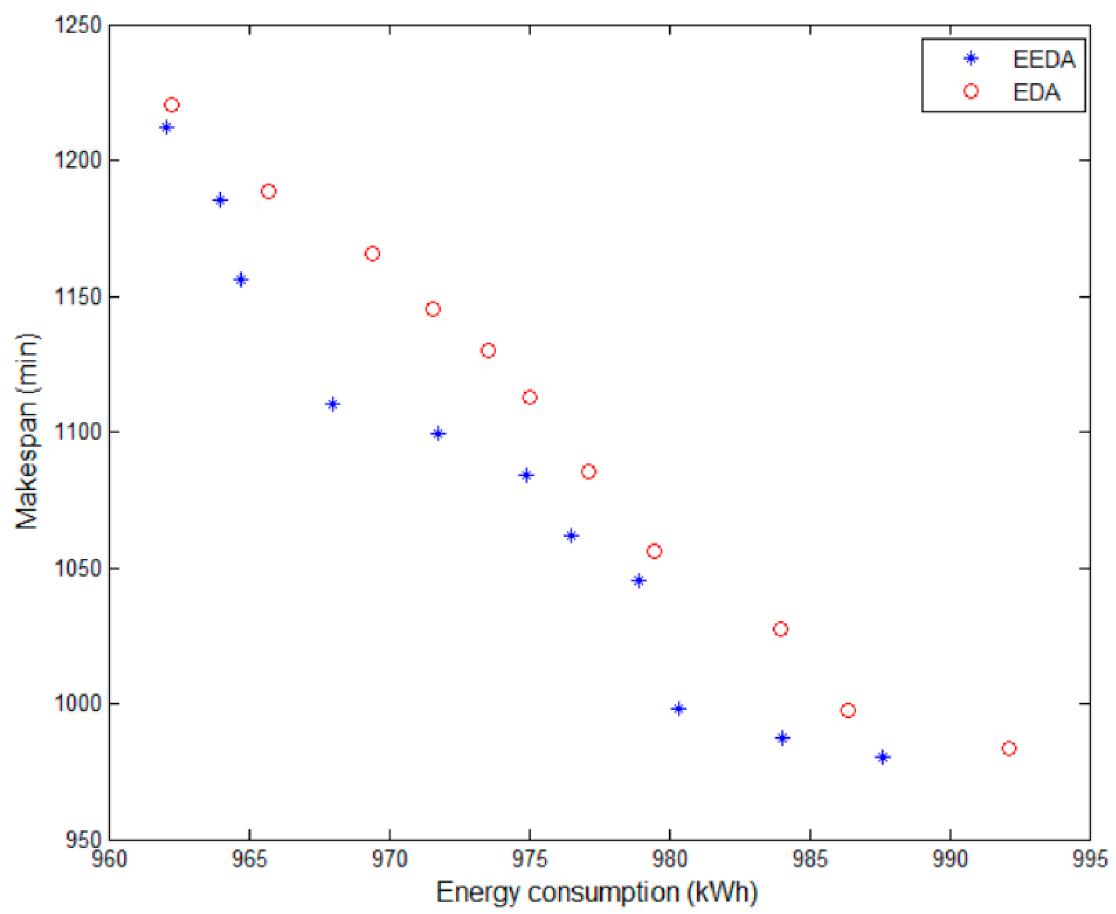
4.3.2. Computational Results on EEDA versus EDA

In order to demonstrate the optimization capability of the EEDA on the potential of the energy savings, the general EDA was also shown as a heuristic strategy. The parameters setting of the EDA was the same as that of the EEDA regarding the population size (NIND), the maximum number of iterations (Maxgen), and the learning rate (α). Due to the fact that the consideration of energy consumption and makespan is different in different manufacturing environments, different weighted importance of energy consumption and makespan should be taken into account in the EJSP. In this section, this is done by changing the value of the weighted importance $w$ with a step size of 0.1. Hence, the objective function is conducted with the weighted importance $w$ from 0 to 1 so that the optimal solutions are from energy-savings oriented to time-savings oriented. The experimental results are shown in

Table 9. Optimization results with different weighted importance on EEDA versus EDA.

w	EEDA			EDA			Solution Gap
	f1	f2	F	f1	f2	F	Gap- f1 (%)	Gap- f2 (%)	Gap- F (%)
0	980.32	987.65	0.0588	992.14	983.42	0.1071	0.32%	0.45%	82.14%
0.1	987.45	984.05	0.0623	986.39	989.28	0.0947	1.00%	0.24%	52.01%
0.2	998.03	980.34	0.0523	987.23	1027.17	0.0874	2.92%	0.38%	67.11%
0.3	1045.17	978.93	0.0607	979.5	1056.36	0.0954	1.07%	0.06%	57.17%
0.4	1061.78	976.52	0.0579	977.16	1085.4	0.0948	2.22%	0.07%	63.73%
0.5	1083.9	974.89	0.0613	975.05	1112.73	0.0983	2.66%	0.02%	60.36%
0.6	1099.06	971.75	0.0688	973.58	1130.22	0.0832	2.84%	0.19%	20.93%
0.7	1110.37	968.02	0.0605	971.6	1145.52	0.1046	3.17%	0.37%	72.89%
0.8	1156.21	964.71	0.0514	969.4	1165.42	0.0983	0.80%	0.49%	91.25%
0.9	1185.53	964.01	0.0677	965.73	1188.23	0.0916	0.23%	0.18%	35.30%
1	1212.32	962.08	0.064	962.25	1220.28	0.1109	0.66%	0.02%	73.28%

.

As seen in Table 9, the comprehensive energy consumption decreased by 25.57 kWh and an optimal energy-efficient schedule result could be obtained by the EEDA. Moreover, the comprehensive energy consumption values obtained by the EEDA had better optimization than EDA, where the average comprehensive energy consumption by EEDA was 0.02% lower than EDA. Moreover, the makespan values from the EDA were larger than those obtained by the EEDA, where the related average gap was 1.62%. Therefore, the optimization effects of the EEDA with regard to the energy consumption and makespan were better than those of the EDA. Meanwhile, the comparison results were given with regard to the makespan and energy consumption with the EEDA and EDA, as demonstrated in Figure 7. It can be observed that the quality of solutions obtained by the EEDA outperformed the quality of solutions obtained by the EDA.

5. Discussion

In summary, the reasonable settings of the parameters in the EEDA had an important impact on the algorithms’ performance. For example, when the population size increased, better individuals could be selected to obtain an optimal solution. However, oversized population sizes will result in more computational time. It is a disadvantage for the EEDA to obtain the best result in a limited time. Hence, it is necessary to design the experiment to determine parameter values, which is shown in Table 2. Furthermore, to verify the effectiveness of the EEDA, experiments with the EEDA versus other algorithms were performed for benchmark problems. According to the results, the EEDA had improvements in solution quality compared to the other algorithms. The reason for this is that the EEDA had a better ability to achieve a balance with the proposed algorithm in both global and local searches.

In addition, the proposed EEDA is a promising method for solving energy-efficient job-shop scheduling problems with transportation constraints. On the one hand, by assessing the algorithm performance, it can be seen that EEDA had a better searching ability compared to other algorithms like the EDA. The reason for this is explained by the EDA being a global search method based on the probability model, but its local search ability is limited. The EEDA is the combination of the EDA and SA, and absorbs their advantages. At the same time, with regard to the local search ability of the SA, it is subject to the constraint of simulated annealing function. A novel annealing schedule method, which is inspired from the hormone modulation mechanism, is designed to achieve the balance of EEDA in both global and local search. On the other hand, through analyzing the optimization capability of the EEDA on the potential of the energy savings in the case study, the EEDA outperforms the EDA in obtaining the optimal solution regarding energy consumption and makespan on a fair basis. It also indicates that the EEDA had the comprehensive search ability.

6. Conclusions

In this study, an energy-efficient job-shop scheduling problem with consideration of AGV transportation was studied. First, a mixed-integer programming model was established to minimize both the comprehensive energy consumption and makespan. Due to the complexity of the problem, the EEDA was designed to explore its optimal solution. Comprehensive experiments were conducted to investigate the proposed model and algorithm. The experimental results indicated that the proposed algorithm was effective in solving the EJSP and it was capable of obtaining better solutions than the EDA. Furthermore, the results highlighted that the transportation energy consumption had a non-negligible impact on the comprehensive energy consumption.

With respect to future work, it will be interesting to study the following issues: (1) the EEDA shows the improvement of algorithm performance compared with other meta-heuristic algorithms, but further research on the model accuracy and computation time should be taken into account; (2) there are many unexpected events such as random machine breakdown, rush task, and task cancellation occurring in practical factories. They may have an influence on the energy consumption, which should be considered in the EJSP. Hence, research on a dynamic integrated scheduling problem for machines and AGVs with consideration of energy consumption should also be studied in the future.

References

1. Wu, X.; Sun, Y. A green scheduling algorithm for flexible job shop with energy-saving measures. J. Clean. Prod. 2018, 172, 3249–3264. [Google Scholar] [CrossRef]
2. Wang, Q.; Tang, D.; Li, S.; Yang, J.; Salido, M.A.; Giret, A.; Zhu, H. An Optimization Approach for the Coordinated Low-Carbon Design of Product Family and Remanufactured Products. Sustainability 2019, 11, 460. [Google Scholar] [CrossRef]
3. Meng, Y.; Yang, Y.; Chung, H.; Lee, P.-H.; Shao, C. Enhancing Sustainability and Energy Efficiency in Smart Factories: A Review. Sustainability 2018, 10, 4779. [Google Scholar] [CrossRef]
4. Gahm, C.; Denz, F.; Dirr, M.; Tuma, A. Energy-efficient scheduling in manufacturing companies: A review and research framework. Eur. J. Oper. Res. 2016, 248, 744–757. [Google Scholar] [CrossRef]
5. Giret, A.; Trentesaux, D.; Prabhu, V. Sustainability in manufacturing operations scheduling: A state of the art review. J. Manuf. Syst. 2015, 37 Pt 1, 126–140. [Google Scholar] [CrossRef]
6. Akbar, M.; Irohara, T. Scheduling for sustainable manufacturing: A review. J. Clean. Prod. 2018, 205, 866–883. [Google Scholar] [CrossRef]
7. Che, A.; Wu, X.; Peng, J.; Yan, P. Energy-efficient bi-objective single-machine scheduling with power-down mechanism. Comp. Oper. Res. 2017, 85, 172–183. [Google Scholar] [CrossRef]
8. Lee, S.; Do Chung, B.; Jeon, H.W.; Chang, J. A dynamic control approach for energy-efficient production scheduling on a single machine under time-varying electricity pricing. J. Clean. Prod. 2017, 165, 552–563. [Google Scholar] [CrossRef]
9. Rubaiee, S.; Yildirim, M.B. An energy-aware multiobjective ant colony algorithm to minimize total completion time and energy cost on a single-machine preemptive scheduling. Comput. Ind. Eng. 2019, 127, 240–252. [Google Scholar] [CrossRef]
10. Zhang, M.; Yan, J.; Zhang, Y.; Yan, S. Optimization for energy-efficient flexible flow shop scheduling under time of use electricity tariffs. Procedia CIRP 2019, 80, 251–256. [Google Scholar] [CrossRef]
11. Li, J.-Q.; Sang, H.-Y.; Han, Y.-Y.; Wang, C.-G.; Gao, K.-Z. Efficient multi-objective optimization algorithm for hybrid flow shop scheduling problems with setup energy consumptions. J. Clean. Prod. 2018, 181, 584–598. [Google Scholar] [CrossRef]
12. Lu, C.; Gao, L.; Li, X.; Pan, Q.; Wang, Q. Energy-efficient permutation flow shop scheduling problem using a hybrid multi-objective backtracking search algorithm. J. Clean. Prod. 2017, 144, 228–238. [Google Scholar] [CrossRef]
13. Fu, Y.; Tian, G.; Fathollahi-Fard, A.M.; Ahmadi, A.; Zhang, C. Stochastic multi-objective modelling and optimization of an energy-conscious distributed permutation flow shop scheduling problem with the total tardiness constraint. J. Clean. Prod. 2019, 226, 515–525. [Google Scholar] [CrossRef]
14. Schulz, S.; Neufeld, J.S.; Buscher, U. A multi-objective iterated local search algorithm for comprehensive energy-aware hybrid flow shop scheduling. J. Clean. Prod. 2019, 224, 421–434. [Google Scholar] [CrossRef]
15. Liu, Y.; Dong, H.; Lohse, N.; Petrovic, S.; Gindy, N. An investigation into minimising total energy consumption and total weighted tardiness in job shops. J. Clean. Prod. 2014, 65, 87–96. [Google Scholar] [CrossRef]
16. Liu, Y.; Dong, H.; Lohse, N.; Petrovic, S. A multi-objective genetic algorithm for optimisation of energy consumption and shop floor production performance. Int. J. Prod. Econ. 2016, 179, 259–272. [Google Scholar] [CrossRef] [Green Version]
17. May, G.K.; Stahl, B.; Taisch, M.; Prabhu, V. Multi-objective genetic algorithm for energy-efficient job shop scheduling. Int. J. Prod. Res. 2015, 53, 7071–7089. [Google Scholar] [CrossRef]
18. Zhang, R.; Chiong, R. Solving the energy-efficient job shop scheduling problem: A multi-objective genetic algorithm with enhanced local search for minimizing the total weighted tardiness and total energy consumption. J. Clean. Prod. 2016, 112, 3361–3375. [Google Scholar] [CrossRef]
19. Salido, M.A.; Escamilla, J.; Giret, A.; Barber, F. A genetic algorithm for energy-efficiency in job-shop scheduling. Int. J. Adv. Manuf. Tech. 2016, 85, 1303–1314. [Google Scholar] [CrossRef]
20. Masmoudi, O.; Delorme, X.; Gianessi, P. Job-shop scheduling problem with energy consideration. Int. J. Prod. Econ. 2019, 216, 12–22. [Google Scholar] [CrossRef]
21. Mokhtari, H.; Hasani, A. An energy-efficient multi-objective optimization for flexible job-shop scheduling problem. Comput. Chem. Eng. 2017, 104, 339–352. [Google Scholar] [CrossRef]
22. Meng, L.; Zhang, C.; Shao, X.; Ren, Y. MILP models for energy-aware flexible job shop scheduling problem. J. Clean. Prod. 2019, 210, 710–723. [Google Scholar] [CrossRef]
23. Dai, M.; Tang, D.; Giret, A.; Salido, M.A. Multi-objective optimization for energy-efficient flexible job shop scheduling problem with transportation constraints. Robot. Comput.-Int. Manuf. 2019, 59, 143–157. [Google Scholar] [CrossRef]
24. Lacomme, P.; Larabi, M.; Tchernev, N. Job-shop based framework for simultaneous scheduling of machines and automated guided vehicles. Int. J. Prod. Econ. 2013, 143, 24–34. [Google Scholar] [CrossRef]
25. Nageswararao, M.; Narayanarao, K.; Ranagajanardhana, G. Simultaneous Scheduling of Machines and AGVs in Flexible Manufacturing System with Minimization of Tardiness Criterion. Procedia Mater. Sci. 2014, 5, 1492–1501. [Google Scholar] [CrossRef] [Green Version]
26. Saidi-Mehrabad, M.; Dehnavi-Arani, S.; Evazabadian, F.; Mahmoodian, V. An Ant Colony Algorithm (ACA) for solving the new integrated model of job shop scheduling and conflict-free routing of AGVs. Comput. Ind. Eng. 2015, 86, 2–13. [Google Scholar] [CrossRef]
27. Guo, Z.; Zhang, D.; Leung, S.Y.S.; Shi, L. A bi-level evolutionary optimization approach for integrated production and transportation scheduling. Appl. Soft. Comput. 2016, 42, 215–228. [Google Scholar] [CrossRef]
28. Karimi, S.; Ardalan, Z.; Naderi, B.; Mohammadi, M. Scheduling flexible job-shops with transportation times: Mathematical models and a hybrid imperialist competitive algorithm. Appl. Math. Model. 2017, 41, 667–682. [Google Scholar] [CrossRef]
29. Liu, Z.; Guo, S.; Wang, L. Integrated green scheduling optimization of flexible job shop and crane transportation considering comprehensive energy consumption. J. Clean. Prod. 2019, 211, 765–786. [Google Scholar] [CrossRef]
30. Tang, D.; Dai, M. Energy-efficient approach to minimizing the energy consumption in an extended job-shop scheduling problem. Chin. J. Mech. Eng. 2015, 28, 1048–1055. [Google Scholar] [CrossRef]
31. Hao, X.; Lin, L.; Gen, M.; Ohno, K. Effective Estimation of Distribution Algorithm for Stochastic Job Shop Scheduling Problem. Procedia. Comput. Sci. 2013, 20, 102–107. [Google Scholar] [CrossRef] [Green Version]
32. Wang, L.; Wang, S.; Xu, Y.; Zhou, G.; Liu, M. A bi-population based estimation of distribution algorithm for the flexible job-shop scheduling problem. Comput. Ind. Eng. 2012, 62, 917–926. [Google Scholar] [CrossRef]
33. Jarboui, B.; Eddaly, M.; Siarry, P. An estimation of distribution algorithm for minimizing the total flowtime in permutation flowshop scheduling problems. Comput. Oper. Res. 2009, 36, 2638–2646. [Google Scholar] [CrossRef]
34. Hauschild, M.; Pelikan, M. An introduction and survey of estimation of distribution algorithms. Swarm. Evol. Comput. 2011, 1, 111–128. [Google Scholar] [CrossRef] [Green Version]
35. Liu, F.; Xie, J.; Liu, S. A method for predicting the energy consumption of the main driving system of a machine tool in a machining process. J. Clean. Prod. 2015, 105, 171–177. [Google Scholar] [CrossRef]
36. Dai, M.; Tang, D.; Giret, A.; Salido, M.A.; Li, W.D. Energy-efficient scheduling for a flexible flow shop using an improved genetic-simulated annealing algorithm. Robot. Comput.-Int. Manuf. 2013, 29, 418–429. [Google Scholar] [CrossRef]
37. Beasley, J.E. OR-Library: Distributing test problems by electronic mail. J. Oper. Res. Soc. 1990, 41, 1069–1072. [Google Scholar] [CrossRef]
38. Fisher, H.; Thompson, G.L. Probabilistic Learning Combinations of Local Job-Shop Scheduling Rules; Prentice-Hall: Englewood Cliffs, NJ, USA, 1963. [Google Scholar]
39. Lawrence, S. Resource Constrained Project Scheduling: An Experimental Investigation of Heuristic Scheduling Techniques (Supplement); Graduate School of Industrial Administration, Carnegie Mellon University: Pittsburgh, PA, USA, 1984. [Google Scholar]
40. He, X.-J.; Zeng, J.-C.; Xue, S.-D.; Wang, L.-F. In an Efficient Estimation of Distribution Algorithm for Job Shop Scheduling Problem. In Swarm, Evolutionary, and Memetic Computing; Panigrahi, B.K., Das, S., Suganthan, P.N., Dash, S.S., Eds.; Springer: Berlin/Heidelberg, Germany, 2010; Volume 6466, pp. 656–663. [Google Scholar]
41. Zhao, F.; Shao, Z.; Wang, J.; Zhang, C. A hybrid differential evolution and estimation of distribution algorithm based on neighbourhood search for job shop scheduling problems. Int. J. Prod. Res. 2016, 54, 1–22. [Google Scholar] [CrossRef]
42. Laarhoven, P.J.M.V.; Aarts, E.H.L.; Lenstra, J.K. Job shop scheduling by simulated annealing. Oper. Res. 1992, 40, 113–125. [Google Scholar] [CrossRef]
43. Wang, L.; Zheng, D.Z. An effective hybrid optimization strategy for job-shop scheduling problems. Comput. Oper. Res. 2001, 28, 585–596. [Google Scholar] [CrossRef]
44. Dorndorf, U.; Pesch, E. Evolution Based Learning in a Job Shop Scheduling Environment. Comput. Oper. Res. 1995, 22, 25–40. [Google Scholar] [CrossRef]
45. Park, B.J.; Choi, H.R.; Kim, H.S. A hybrid genetic algorithm for the job shop scheduling problems. Comput. Ind. Eng. 2003, 45, 597–613. [Google Scholar] [CrossRef]
Figure 1. An example schedule.
Sustainability 11 03085 g001
Figure 2. Constraints of two successive operations for a task.
Sustainability 11 03085 g002
Figure 3. Parameters’ influence on the average makespan.
Sustainability 11 03085 g003
Figure 4. Breakdown of energy consumption of different transportation speeds for w = 0.
Sustainability 11 03085 g004
Figure 5. Breakdown of energy consumption of different transportation speeds for w = 0.5.
Sustainability 11 03085 g005
Figure 6. Breakdown of energy consumption of different transportation speeds for w = 1.
Sustainability 11 03085 g006
Figure 7. Distribution of solutions with different weighted importance on the EEDA versus EDA.
Sustainability 11 03085 g007