A New Equation to Evaluate Liquefaction Triggering Using the Response Surface Method and Parametric Sensitivity Analysis

Abstract

Liquefaction is one of the most damaging functions of earthquakes in saturated sandy soil. Therefore, clearly advancing the assessment of this phenomenon is one of the key points for the geotechnical profession for sustainable development. This study presents a new equation to evaluate the potential of liquefaction (PL) in sandy soil. It accounts for two new earthquake parameters: standardized cumulative absolute velocity and closest distance from the site to the rupture surface (CAV₅ and r_rup) to the database. In the first step, an artificial neural network (ANN) model is developed. Additionally, a new response surface method (RSM) tool that shows the correlation between the input parameters and the target is applied to derive an equation. Then, the RSM equation and ANN model results are compared with those of the other available models to show their validity and capability. Finally, according the uncertainty in the considered parameters, sensitivity analysis is performed through Monte Carlo simulation (MCS) to show the effect of the parameters and their uncertainties on PL. The main advantage of this research is its consideration of the direct influence of the most important parameters, particularly earthquake characteristics, on liquefaction, thus making it possible to conduct parametric sensitivity analysis and show the direct impact of the parameters and their uncertainties on the PL. The results indicate that among the earthquake parameters, CAV₅ has the highest effect on PL. Also, the RSM and ANN models predict PL with considerable accuracy.

1. Introduction

Nowadays, it is crucially important for engineers and urban planners to take sustainability, livability, and social health into account when considering natural disasters. The sustainability framework includes principles of sustainability in conjunction with hazard mitigation. Further, evaluating hazards and revising plans are two of the main steps of the classic planning approach [1].

The subject of liquefaction started to garner a great deal of attention after two major earthquakes caused mortality and substantial damage in 1964. Massive landslides happened due to the liquefaction that occurred during the Alaska earthquake, which had a magnitude of 9.2 on the Richter scale, and demolished more than 200 bridges. During the Niigata earthquake, which had a magnitude of 7.5 on the Richter scale, excessive liquefaction caused major damage to more than 60,000 buildings and bridges, highways, and other urban city constructions. Liquefaction poses major threats to the sustainability of existing lifestyles.

Liquefaction occurs in saturated sandy soil due to the dynamic loads that occur during earthquakes. The rapid loads do not allow drainage, so pore water pressure increases, while at the same time effective stress goes down to be zero, or close to zero. Consequently, soil loses its shear strength, and liquefaction happens.

After several decades of intensive research on liquefaction, researchers have presented a variety of methods based on three approaches to evaluate its potential. These three approaches are (1) energy-based [2,3,4,5,6,7,8,9,10,11,12], (2) cyclic stress-based [13,14,15,16,17,18,19,20], and (3) strain-based [8,9,10,11,21,22,23,24,25,26]. The energy-based models estimate the energy that is dissipated into the soil by earthquake loads. In the stress-based method, first, the cyclic stress ratio (CSR) and cyclic shear strength (CRR) are calculated; then, the potential of liquefaction is evaluated by comparing them. The strain-based models suppose that the cyclic shear strain loads control the increase in the pore water pressure. Empirical and semi-empirical methods based on the stress-based approach are more popular among researchers [14,27,28]. Seed and Idriss [29] developed a semi-empirical equation for the earthquake load by calculating the uniform cyclic shear stress amplitude.

Moreover, to determine soil liquefaction resistance, two types of methods have been used to measure the cyclic resistance ratio (CRR) and then compare it with the cyclic stress ratio (CSR): laboratory test-based methods and in situ test-based methods.

Some studies, such as those of Robertson and Wride [13], Youd et al. [14], Juang et al. [27], and Rezania et al. [28], have conducted deterministic analysis to calculate the factor of safety (FS), but due to uncertainty in the liquefaction phenomena, some other researchers have performed probabilistic analysis [7,16,27,30,31,32,33,34,35]. Artificial neural network (ANN) is a strong technique in cases with non-linear correlations between parameters, such as the liquefaction phenomena. Hence, ANN has been used to investigate this issue [31,36,37,38]. However, the data division is conducted randomly in two groups for the testing and training phase, and there is no validating phase to prevent over-training the model. The validating phase is applied to minimize the over-fitting of the trained model. If the accuracy of the training dataset goes up, but the accuracy of the validation dataset decreases, then over-fitting occurs, and the training should be stopped. Goh [36] was the first to use a simple back-propagation ANN algorithm to find the relationship between the soil and seismic parameters, and the liquefaction potential. He examined the following eight parameters: SPT value (N_1,60), fines content (FC), mean grain size (D50), equivalent dynamic shear stress (τ_av/σ’_v), σ_v, σ’_v, Mw, and peak horizontal ground acceleration (PGA). His results showed that N_1,60 and FC are the most influential parameters, and he compared his ANN results with those of Seed et al. [39]. In another study, Baziar and Nilipour [38] used STATISCA neural networks to evaluate the potential of liquefaction. They confirmed that neural networks (NN) are a capable tool for analyzing liquefaction.

Applying fuzzy neural network models to predict liquefaction, Rahman and Wang [40] considered nine parameters: magnitude of the earthquake (M), vertical total overburden pressure, vertical effective overburden pressure, q_c1N value from CPT, acceleration ratio PGA/g, CSR, median grain diameter of the soil, critical depth of liquefaction, and water table depth. They combined fuzzy systems and NN to use both systems’ advantages: the learning and optimization ability of NN, and the human-like analysis of the fuzzy system to consider the meaning of high, very high, or low. Their databases included 205 field liquefaction records from more than 20 major earthquakes between 1802–1990. On the other hand, Hanna et al. [31] used the generalized regression neural network (GRNN) to find the liquefaction potential of soil. They considered 12 soil and seismic parameters from the two earthquakes that occurred in Turkey and Taiwan.

All in all, ANN models that assess the potential of liquefaction are still lacking. A validating phase is missing to prevent the model from overtraining. Furthermore, data division has been performed randomly without attention to statistical aspects of the databases.

According to Kramer and Mitchell [41], the ground motion caused by earthquakes can be affected by an earthquake’s fault type characteristics. Furthermore, the stress energy carried by earthquake waves decreases exponentially with epicentral distance (R_epi). Takahashi et al. [42] investigated the influence of the faulting mechanism on the motions caused by earthquakes, and defined, for example, reverse faulting in comparison with strike-slip and normal faulting shows around 30% higher spectra acceleration. Furthermore, near-fault zones experienced high peak horizontal ground acceleration (PGA) with high frequency and a short period, with a less active load on structures [43] and no liquefaction occurrence [44,45]. In an investigation of large-scale Japanese earthquakes, Orense [45] discovered some seismic records in Japan with a high frequency. Even with large acceleration, he observed no liquefaction. Therefore, he proposed the threshold for peak ground velocity (PGV) and PGA for the occurrence of liquefaction. Furthermore, Liyanapathirana and Poulos [44] analyzed some earthquakes from all around the world and compared them with characteristics of Australian earthquakes. They indicated that the low value of cumulative absolute velocity (CAV of Australian earthquakes, which is the time integration of the absolute values of the acceleration, is the key reason for their lack of liquefaction, even with high PGA.

It has been demonstrated that the earthquake intensity measure (IM) with the best combination of efficiency and sufficiency is standardized cumulative absolute velocity (CAV₅) [41,44]. However, no study has explored its influence and correlation with liquefaction in empirical or semi-empirical models. Furthermore, to the best of the present authors’ knowledge, the studies that have been performed did not take into account the effectiveness of parameters and their uncertainties, according to the use of CRR and CSR, on the triggering of liquefaction.

In this study, the most essential parameters to evaluate the potential of liquefaction are selected according to background research studies [7,13,15,16,27,28,30,31,46,47,48,49,50]. Then, two new earthquake parameters added to the dataset to create a comprehensive database: CAV₅ and the closest distance from the site to the rupture surface (r_rup). So, strict consideration was given to the earthquake parameters in addition to the soil properties and geometry of the sites. The new earthquake parameters (CAV₅ and r_rup) were estimated through attenuation equations derived by Kramer and Mitchell [41] and Sadigh et al. [51], respectively. Consequently, this study considers the influence of earthquakes’ causative fault type, the effect of earthquakes near the fault zone, and the frequency of earthquakes’ load. In the first step, data are collected to develop an ANN model. To achieve this goal, the data are divided by considering their statistical aspects instead of random division. Furthermore, the data are divided into three groups for the training, testing, and validating phase to prevent the overtraining of the model.

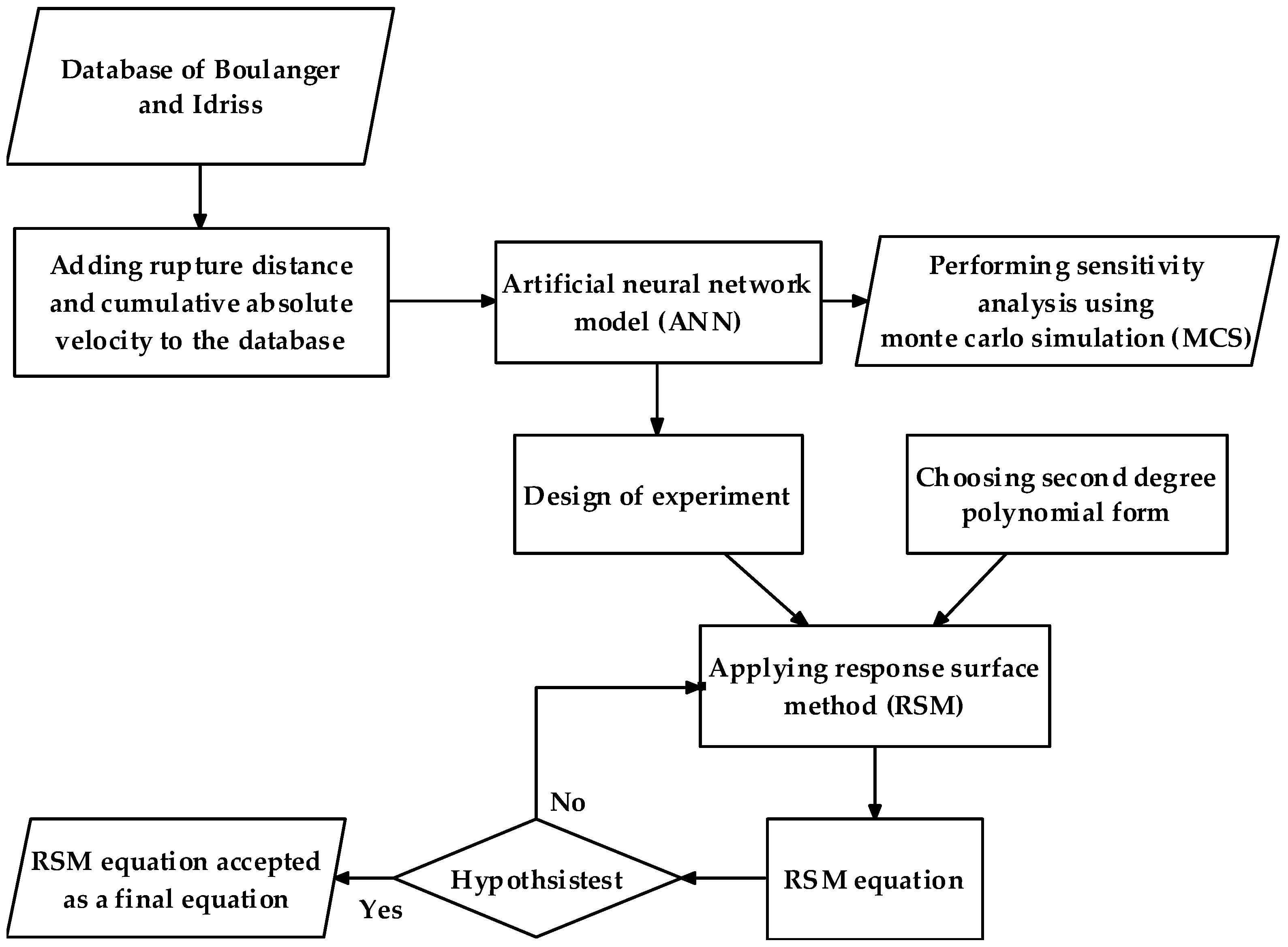
Then, the design of experiment (DOE) is conducted to cover all of the ranges of parameters by points. The ANN model is applied to estimate the target of DOE sample points. Subsequently, the response surface method (RSM), which is a novel method regarding risk assessment and the hazard analysis of liquefaction, is used to establish a direct equation to evaluate the triggering of liquefaction instead of using CRR and CSR. This makes is easier for engineers and contractors to use. Finally, due to uncertainties in soil properties and earthquake parameters, on the basis of the ANN model that was developed in this study and through Monte Carlo simulation (MCS), sensitivity analysis is performed to show the effect of the parameters and their uncertainties on the potential of liquefaction in sandy soils. In Section 8, the proposed model to evaluate the potential for liquefaction triggering (PL) is described. The developed ANN and RSM models are presented in Section 9. The capability and accuracy of the models are confirmed by comparing their results with three extra well-known models. Finally, the sensitivity analysis results are illustrated in 10 graphs. Figure 1 illustrates the flowchart of the risk assessment performed in this study to evaluate PL and conducting sensitivity analysis.

2. Analysis Methods

The liquefaction triggering analyses were carried out by comparing the strength of soil against the liquefaction or cyclic strength ratio (CRR) with the stress-loading effects or cyclic stress ratio (CSR). Section 2.1 and Section 2.2 state the methods that have been defined by research studies.

2.1. Deterministic Methods

Through deterministic methods, the liquefaction potential is expressed as a factor of safety (FS), which is the ratio of CRR to CSR, without considering the uncertainty associated with the loading and resistance predictions. Robertson and Wride [13] divided the cone penetration test result range in two parts, and presented two equations for CRR:

$${CRR}_{7.5}=0.833\left[\frac{q_{c1N,CS}}{1000}\right]+0.05 \mathrm{for} q_{c1N,cs}<50$$

(1a)

$${CRR}_{7.5}=93{\left[\frac{q_{c1N,cs}}{1000}\right]}^3+0.08 \mathrm{for} 50\le q_{c1N,cs}<160$$

(1b)

$$q_{c1N,cs}=K_1{q}_{c1N}$$

(1c)

$$K_1=2.429{\left(I_c\right)}^4-16.943{\left(I_c\right)}^3+44.551{\left(I_c\right)}^2-51.497\left(I_c\right)+22.802$$

(1d)

$$q_{c1N}=\frac{q_c/100}{{({\sigma }_v^{\prime }/100)}^{0.5}}$$

(1e)

where I_c is the soil type index, σ_v’ is the effective stress, and q_c1N is defined as above [13].

Youd et al. [14] presented the following relation for the measurement of FS in which $K_{\sigma }$ is the overburden correction factor, $K_{\alpha }$ is the factor of static shear stress correction, and $MSF$ is the magnitude scaling factor.

$$FS=(CR{R}_{7.5}/CSR)·MSF·K_{\sigma }·K_{\alpha }$$

(2)

Juang et al. [27] generated artificial boundary points between a liquefied and a non-liquefied area onto a two-dimensional (2D) surface of CSR and CRR through a trained neural network. Then, they developed an empirical equation by regression analysis to present the limit state function as follows:

$$CRR=C_{\sigma }exp\left[-2.957+1.264(\frac{q_{c1N,cs}}{100}{)}^{1.25}\right]$$

(3a)

where:

$$C_{\sigma }=-0.016{\left(\frac{{\sigma }_v^{\prime }}{100}\right)}^3+0.178{\left(\frac{{\sigma }_v^{\prime }}{100}\right)}^2-0.063\left(\frac{{\sigma }_v^{\prime }}{100}\right)+0.903$$

(3b)

Idriss and Boulanger [15] updated semi-empirical field-based procedures for evaluating the liquefaction potential of cohesionless soils during earthquakes. They re-examined the field data and updated the analytical framework, and presented standard penetration test results-based (SPT-based) and cone penetration test results-based (CPT-based) liquefaction correlations for cohesionless soils. Moreover, they developed a new equation:

$$CR{R}_{7.5}=exp\left\{\frac{{(N_1)}_{60cs}}{14.1}+{\left(\frac{{(N_1)}_{60cs}}{126}\right)}^2-{\left(\frac{{\left(N\right)}_{60cs}}{23.6}\right)}^3+{\left(\frac{{\left(N\right)}_{60cs}}{25.4}\right)}^4-2.8\right\}$$

(4)

By applying evolutionary polynomial regression (EPR), Rezania et al. [28] developed a model as a three-dimensional (3D) surface boundary to evaluate the potential for liquefaction:

$$CRR=exp\left[-6.994+7.9\ast {10}^{-6}{q}_{c1N}^{2.5}+1.115\ast Ln\left({\sigma }_v^{\prime }\right)\right]$$

(5)

The essential influence of the CPT test results on the potential for liquefaction has been illustrated in all of the defined models in this section.

2.2. Probabilistic Models

Due to uncertainties in soil properties, earthquake parameters, and models, $FS>1$ does not always reveal non-liquefaction. Similarly, $FS\le 1$ does not always correspond to the occurrence of liquefaction. In the records of Seed and Idriss [29] and Zhou and Zhang [52], there are 40 data points of 12 earthquakes that occurred in the time period of 1802–1976, among which 27 sites liquefied and 13 sites did not. Zhang et al. [46] considered the following five factors: magnitude of the earthquake (M), source distance (L), depth of the water table, depth of the sand deposit, and SPT blow count (N). Using the optimum-seeking method, the authors evaluated the liquefaction and influence of these five factors, and declared that the most effective parameters are SPT blow count (N) and the magnitude of the earthquake. Toprak et al. [30] analyzed a total of 79 data points of SPT by logistic regression. Fifty data points were from the 1989 Loma Prieta, California earthquake, and 29 data points were from the 1971 San Fernando, the 1979 Imperial, the 1987 Superstition Hills, and the 1994 Northridge earthquakes. They presented the following equation to estimate the potential for liquefaction (P_L):

$$\ln \left[P_L/1-P_L\right]=13.6203-0.2820{\left(N_1\right)}_{60,cs}+5.3265\ln \left(CS{R}_{7.5}\right)$$

(6)

They also analyzed 48 data points from the United States (US) Geological Survey from the 1989 Loma Prieta earthquake by the logistic regression analysis of CPT, and presented the following equation:

$$\ln \left[P_L/1-P_L\right]=12.260-0.0567q_{C1N,cs}+4.0817\ln \left(CS{R}_{7.5}\right)$$

(7)

where CSR_7.5 is the coefficient of the earthquake magnitude scale.

Chen et al. [7] presented two models for liquefaction by using seismic wave energy. They also used discriminate analysis with normal distribution and demonstrated the ability of this distribution to assess liquefaction potential. They presented the equations by using data collected from the Chi-Chi earthquake.

3. Attenuation Equations for Standardized Cumulative Absolute Velocity and Peak Ground Acceleration

Kramer and Mitchell [41] executed the regressive project to evaluate the influence of approximately 300 earthquake intensities (IMs) on the liquefaction. Their database contained more than 450 ground motions from 22 earthquakes. They stated that the IM with the best combination of efficiency and sufficiency is the cumulative absolute velocity with a threshold value of 5 cm/s², which is shown as CAV₅ (Equation (8)). Furthermore, they developed an attenuation equation to estimate CAV₅ as follows:

$${CAV}_5={\displaystyle {\int }_0^{\infty }}\alpha \left|a_{\left(t\right)}\right|dt\mathrm{where}\alpha =\{\begin{array}{l}0\mathrm{for} \left|a_{\left(t\right)}\right|<5 \mathrm{cm}/{\mathrm{s}}^2\\ 1\mathrm{for} \left|a_{\left(t\right)}\right|\ge 5 \mathrm{cm}/{\mathrm{s}}^2\end{array}$$

(8)

$$\ln {CAV}_5=C_1+C_2\left(M-6\right)+C_3\ln (M/6)+C_4\ln (\sqrt{r_{rup}{}^2+h^2})+f_1{F}_N+f_2{F}_R$$

(9)

The coefficients of the regression are C₁ = 3.495, C₂ = 2.764, C₃ = 8.539, C₄ = 1.008, f₁ = 0.464, f₂ = 0.165, and h = 6.155. The coefficients of the three fault types are given by:

Strike-slip (F_N = F_R = 0), normal faults (F_N = 1 and F_R = 0), and reverse or reverse-oblique (F_N = 0 and F_R = 1)

Sadigh et al. [51] used a strong motion database of California earthquakes for strike-slip and reverse causative fault with magnitudes of four to more than eight, and r_rup of up to 100 km. Based on this, they presented the following attenuation equation for rock and deep firm soil deposits:

$$\ln \left(\mathrm{PGA}\right)=C_1+C_{2}M-C_3\ln (r_{rup}+C_4{e}^{C_{5}M})+C_7{\left(8.5-M\right)}^{2.5}$$

(10)

where C₁ is an indicator of the causative fault type, the strike-slip value is −2.17, and the value of the reverse and thrust faults is −1.92.

• C₂ = 1.0, C₃ = 1.70, C₆ = 0
• C₄ = 2.1863, C₅ = 0.32 for M ≤ 6.5
• C₄ = 0.3825, C₅ = 0.5882 for M > 6.5

4. Artificial Neural Network

In cases that exhibit non-linear relationships between input and output parameters, an ANN is often used in research. This technique simulates biological neuron processing in the human brain with simple artificial neuron connections. McCulloch et al. [53] were the first to present neural networks. After that, numerous researchers applied this technique. Multi-layer perceptron (MLP) [54], which is employed in the present study, is the most commonly used. The back-propagation network is the most popular among the MLP paradigms. A MLP contains three types of layers, which include: an input layer, a hidden layer, and an output layer or layers. However, it has been demonstrated that a single hidden layer is sufficient for non-linear analysis. There can be more than one hidden layer; however, theoretical works have shown that a single hidden layer is sufficient for MLP to approximate any complex non-linear function [55]. Therefore, an MLP with three layers and a single hidden layer is applied in the present study to predict the target.

There are three indicators to justify ANN: the root of the mean squared error (RMSE), the coefficient of determination (R²), and the mean absolute error (MAE). However, R² is the most common, and it is considered herein as:

$$R^2=1-(\frac{{\sum }_{i=1}^n{\left(Y_{Estimated}-Y_{Measured}\right)}^2}{{\sum }_{i=1}^n{\left(Y_{Measured}\right)}^2})$$

(11)

5. Response Surface Methodology

The response surface method (RSM) consists of some statistical techniques, and supports Taguchi’s philosophy [56] regarding mathematical processes to build a model and optimize a response. In the present study, the RSM is applied to establish a correlation between parameters. To achieve this goal, three main steps were followed:

• Choosing a reasonable design of experiment (DOE).
• Selecting an approximate mathematical form.
• Determining the significance of equation terms through hypothesis testing.

The first step is choosing a sampling point or experimental design. There are several kinds of DOE techniques, such as central composite design, minimum design, D-optimal designs, full factorial design, Taguchi’s contribution design, star design, and Latin hypercube design. In this study, to examine a range of parameters and prevent a negative value in the DOE [57], the design of Box and Behnken [58] is applied. Furthermore, to find the sampling point space, an ANN is applied. According to the DOE and 10 input parameters, 170 sample points are produced by the RSM. To estimate the target (response) of these samples, which is called a coded value here, an ANN model that was trained with a case history database was applied. The coded values for any sample are as follows: The Max value is supposed to be (+1), the mean value is supposed to be (0), and the Min value is supposed to be (−1).

The second step of a RSM is choosing a suitable approximation form to present the relationship between the target (response) and inputs. This is the difference between the RSM and genetic programming.

The most common response surface form that researchers use is polynomial forms, which are given by:

$$R_{\left(X\right)}=a_0+{\sum }_{i=1}^n{b}_i{X}_i, \text{first-degree} \mathrm{polynomial}$$

(12)

$$R_{\left(X\right)}={\sum }_{i=1}^n{b}_i{X}_i+{\sum }_{i=1}^n{C}_i{X}_i{}^2, \text{second-degree} \mathrm{polynomial} \mathrm{without} \mathrm{cross} \mathrm{terms}$$

(13)

$$R_{\left(X\right)}=a_0+{\sum }_{i=1}^n{b}_i{X}_i+{\sum }_{i=1}^n{C}_i{X}_i{}^2+{\sum }_{\begin{array}{c}i=1\\ j\ne i\end{array}}^n{d}_{ij}{X}_i{X}_j, \text{second-degree} \mathrm{polynomial} \mathrm{with} \mathrm{cross} \mathrm{terms}.$$

(14)

To identify significant terms in the equation, a hypothesis test is conducted in the last step. A hypothesis test evaluates the terms relating to a population to determine which terms are the best supported by the sample data. By considering the p-value, some expressions are eliminated in order to achieve the most effective and meaningful terms to build the final equation.

It is common to use hypothesis testing based on p-values in statistics such as basic statistics, linear models, reliability, and multivariate analysis. The p-values have a range from 0 to 1, and show the probability of obtaining a test statistic that is at least as extreme as the calculated value when the null hypothesis is correct.

6. Monte Carlo Method

Researchers have used the Monte Carlo method to study both stochastic and deterministic systems [59,60,61,62,63,64,65]. It is a useful technic for both linear and non-linear systems. The only problem making it awkward to use is that it requires too large a number of simulations to present a reliable distribution of the response.

Monte Carlo methods can be divided into two general applications: first, the stochastic generation of samples; and second, solving problems that are too complicated to solve through analytical methods. The latter is done by generating suitable random (or pseudo-random) numbers and calculating the ratio of the numbers that have the same properties to all of the numbers.

Jha and Suzuki [33] compared the first-order second-moment (FOSM) method, the point estimation method (PEM), and a Monte Carlo simulation (MCS) method, and also presented a combined method using both FOSM and PEM to find the probability of liquefaction. They showed that the safety factor of the potential for liquefaction that was obtained from the combined method was similar to the results from MCS.

7. Case History Database

This study uses an updated version of the liquefaction CPT database case histories from Boulanger and Idriss [19]. It contains a total of 253 cases in which I_C < 2.6. I_C is the soil behavior type index presented by Robertson and Wride [13] to classify soils based on fine content. The index ranges from 0.5 for sands to 1.0 for clays, and is given by:

$$I_c={\left[{(3.47-\log \left(Q\right))}^2+{(1.22+\log \left(F\right))}^2\right]}^{0.5}$$

(15)

where:

$$Q=\left(\frac{q_c-{\sigma }_v}{P_a}\right){\left(\frac{P_a}{{{\sigma }^{\prime }}_v}\right)}^n, (Q)\text{ is normalized tip ratio}$$

(16)

$$F=\left(\frac{f_s}{q_c-{\sigma }_v}\right)·100\%, \left(F\right) \mathrm{is} \mathrm{normalized} \mathrm{sleeve} \mathrm{friction} \mathrm{ratio}$$

(17)

Of all cases, 180 contained surface evidence of liquefaction, 71 cases did not, and two included doubtful evidence. The common I_c border value of 2.6 [13] is applied to eliminate soils with a clay treatment; therefore, the 15 cases with I_c ≥ 2.6 are not used in this study. Around 30% of all of the samples belonged to the 1989 Loma Prieta earthquake, including 76 case history samples. The map of liquefaction and its associated effects can be seen in Appendix A and Appendix B, in the southern part and the northern part, respectively. Next to that, Appendix C illustrates the locations of the ground failure and damage to the facilities on Treasure Island that were attributed to the 1989 Loma Prieta earthquake. These figures illustrate the ground failure sites, lateral spread, ground settlement, sand boil points, and cracks that were caused by liquefaction in this area.

The dataset contains two earthquake parameters: moment magnitudes (Mw) and PGA. Given that the purpose of this study is to consider the new earthquake parameters (CAV₅ and r_rup), Kramer et al.’s [41] equation is used. Due to the shortage of known parameters to apply this equation, the causative faulting mechanism of all of the earthquakes in the dataset is first characterized to utilize both equations. Then, Sadigh et al.’s [51] attenuation equation is applied to estimate the r_rup. Next to that, due to the magnitude range of the attenuation equations, the seven data samples from the Tohoku earthquake, with a moment magnitude of nine, are eliminated from the dataset. From all of the parameters in the source, only eight are selected according to studies reported in the literature [7,13,15,16,27,28,30,31,46,47,48,49,50]: momentum magnitude (Mw), PGA(g), thickness of liquefiable soil (m) (measured from critical depth interval)(T), ground water table GWT (m), overburden stress (σ) (kPa), effective overburden stress (σ’) (kPa), normalized con penetration test result tip (q_c1N), mean grain size (D₅₀), and fine content (FC) (%). The two extra parameters of CAV and r_rup are added to the dataset through Equations (9) and (10) Therefore, the study considers some of the essential aspects of the earthquakes, such as the near-fault earthquake zone and causative fault type of the earthquake. The summary of the dataset that is used in this study can be seen in

Table 1. Summary of dataset used in this study. NZ: New Zealand, US: United States.

Earthquake	Total Data No.	Train Data No.	Test Data No.	Validation Data
Liquefied Sites
1983 M = 6.9 Borah Peak, US	4	2	1	1
1999 M = 7.6 Chi-Chi, Taiwan	11	7	2	2
2011 M = 6.2 Christchurch, NZ	21	13	4	4
2010 M = 7.1 Darfield, NZ	18	12	3	3
1987 M = 6.6 Edgecumbe, NZ	12	8	2	2
1995 M = 6.9 Hyogoken-Nambu, Japan	16	10	3	3
1979 M = 6.5 Imperial Valley, US	2	2	0	0
1968M = 7.2 Inangahua, NZ	2	2	0	0
1999 M = 7.5 Kocael, Turkey	14	8	3	3
1989 M = 6.9 Loma Prieta, US	49	29	10	10
1983 M = 7.7 Nihonkai Chub, Japan	2	2	0	0
1964 M = 7.6 Niigata, Japan	2	2	0	0
1994 M = 6.7 Northridge, US	2	2	0	0
1987 M = 6.5 Superstition Hills, US	1	1	0	0
1976 M = 7.6 Tangshan, China	13	9	2	2
1980 M = 6.3 Victoria (Mexicali), US	4	2	1	1
1981 M = 5.9 West Morland, US	3	1	1	1
Total	176	112	32	32
Doubtful Sites
1975 M = 7.0 Haicheng, China	1	1	0	0
1989 M = 6.9 Loma Prieta, US	1	1	0	0
Total No.	2	2	0	0
Non-Liquefied Sites
2011 M = 6.2 Christchurch, NZ	4	4	0	0
2010 M = 7.1 Darfield, NZ	7	5	1	1
1987 M = 6.6 Edgecumbe, NZ	5	3	1	1
1975 M = 7.0 Haicheng, china	1	1	0	0
1995 M = 6.9 Hyogoken-Nambu, Japan	7	3	2	2
1979 M = 6.5 Imperial Valley, US	2	2	0	0
1999 M = 7.5 Kocaeli, Turkey	1	1	0	0
1989 M = 6.9 Loma Prieta, US	26	14	6	6
1983 M = 7.7 Nihonkai-Chubu, Japan	1	1	0	0
1964 M = 7.6 Niigata, Japan	1	1	0	0
1987 M = 6.5 Superstition Hills, US	5	3	1	1
1976 M = 7.6 Tangshan, China	6	4	1	1
1981 M = 5.9 West Morland, US	2	2	0	0
Total No.	68	44	12	12

.

8. Proposed Model and Equation to Evaluate Liquefaction Triggering

The dataset that was collected for this study is illustrated in Table 1. As can be seen, it includes 246 samples: 68 non-liquefied samples, 176 liquefied samples, and two doubtful samples [19]. The same portion of liquefied and non-liquefied samples is selected for division, instead of a randomness division. As can be seen from Table 1, around 18% of the liquefied samples, or 32 samples, are selected for the ANN testing phase, and an equal number is selected for the validating phase. A similar ratio of non-liquefied samples is chosen, too. Twelve samples from a total of 68 are chosen for testing, and an equal number is selected for the validating phase.

Furthermore, the parameters are divided into three parts based on similar statistical characteristics, such as the mean value and mean coefficient of variation (COV), in order to increase the accuracy and capability of the trained model. Single hidden layer neural network training was developed in conjunction with the back-propagation algorithm to train a model [36,37,38]. In addition, the ANN target to evaluate the potential for liquefaction according to the dataset is introduced as:

$$T=\{\begin{array}{l}1for liquefied cases\\ 0.5for doubtful cases\\ 0for non-liquefied cases\end{array}$$

(18)

The new equation is presented by applying the new tool for the response surface method (RSM). To the best of the authors’ knowledge, no approach has yet used this tool to assess liquefaction in sandy soil. In the present study, the RSM is applied to develop correlations between the input parameters and the target. The ANN model is used to calculate the coded points, which are defined in Section 4. The new equation presented herein has two advantages over the processes and models that have been presented by other researchers:

• Some aspects of earthquakes, such as the near-fault sites and the frequency content of earthquake motions, are considered by exploring and adding the two new parameters of CAV₅ and r_rup.
• Since it uses direct parameters instead of just CRR and CSR, it is simpler to use in projects by engineers and city planners to obtain sustainable design.

Since the equation uses direct parameters, extra statistical and probabilistic aspects are considered during sensitivity analysis. In contrast, when analyzing liquefaction through CRR and CSR, it is only possible to consider model uncertainty, not parameter uncertainties.

In this study, the second-degree polynomial with cross terms (Equation (14)), which is the most frequently utilized form, is applied to derive a final equation. The alpha (α) level of 0.05 is commonly used by scientists and researchers, and is considered herein. This means that if the p-value of a test statistic is less than alpha, which is herein 0.05, then the null hypothesis is rejected. Here, the null hypothesis is that there is no meaningful correlation between the input value and the target, so the expressions with a P-value of more than 0.05 are eliminated. Furthermore, according to Equation (18), the following values are supposed to evaluate the results of an ANN and the RSM:

$$\begin{array}{c}T<0.4Non-liquefied\\ T>0.6Liquefied\\ 0.4\le T\le 0.6Doubt \left(No acceptable result\right)\end{array}$$

(19)

9. Results

The developed ANN model is applied to measure the coded values of the DOE of the RSM, and is the basis of the sensitivity analysis using MCS. As illustrated in

Table 2. Statistical aspects of variables.

Statistical Parameters
Input Variable	Mean	Std. Dev.	Min	Max	Mean	Distribution Function	References
					COV
Mw	6.8	0.51	5.9	7.7	0.075	Normal distribution	[66]
PGA	0.465	0.06975	0.09	0.84	0.15	Normal distribution	[66]
rrup	26.23	0	1	51.46	0	No uncertainty	*
CAV5	29.78	2.978	1.2	58.36	0.1	Normal distribution	*
T	3.25	0	0.3	6.2	0	No uncertainty	*
GW	3.7	0	0.2	7.2	0	No uncertainty	*
σv	117	17.55	24	210	0.1	Normal distribution	[66]
σ’v	83	12.45	19	147	0.15	Normal distribution	[66]
FC	42.5	8.5	0	85	0.3	Normal distribution	[67]
qc1N	162.7	32.54	13.6	311.8	0.2	Normal distribution	[68]

r_rup, T and GW are supposed as a parameter and no variable. CAV is supposed variable with COV of 0.1 less than COV supposed for PGA [41] *.

, 10 parameters are considered as input parameters, including earthquake parameters, geometry parameters, and soil properties. The target is introduced by Equation (19).

Table 3. Correlation Coefficient of ANN model.

Total Data	Testing Data	Validating Data	Training Data
76.2	80.4	70	78

illustrates the certificate of the ANN model. In the second step, the target values of the DOE samples are predicted through the developed ANN model. In the third step, RSM analysis is performed to derive an equation. The second-degree polynomial with cross terms, which is the most complicated general equation and has the best capability and accuracy, and is illustrated in Equation (14), is utilized to present an equation that relates the 10 input parameters (as a coded value by DOE) and the response values (measured through ANN). Finally, MCS is applied to conduct a sensitivity analysis to demonstrate the influence of the parameters and their uncertainties on the probability of triggering liquefaction (PL) in sandy soil caused by earthquake motions.

9.1. RSM Equation to Evaluate Liquefaction Triggering

In the first analysis using the RSM, the first generated equation has all of the expressions (terms) of the general equation. It contains 66 expressions, but using the hypothesis test, those with a p-value greater than 0.05 are eliminated. Then, the RSM analysis is performed repeatedly until the final equation is presented by 49 expressions, according to

Table 4. Final RSM equation to evaluate the liquefaction potential.

Term	Constant	Mw	PGA	rrup	CAV5	T	GWT
Coefficient	0.12	0.074	0.611	0.098	1.41 × 10−5	−0.13	0.167
Term	σ	σ’	FC	qc1N	PGA*PGA	σ’*σ’	FC*FC
Coefficient	0.20	−0.159	0.181	−0.593	−0.364	0.09	0.214
Term	qc1N*qc1N	M*PGA	Mw*rrup	Mw*CAV5	Mw*T	Mw*GWT	Mw*σ’
Coefficient	0.181	−0.194	0.257	0.228	−0.107	−0.113	0.107
Term	Mw*FC	Mw*qc1N	PGA*rrup	PGA*CAV5	PGA*T	PGA*GWT	PGA*σ
Coefficient	0.174	−0.267	0.313	0.347	0.254	−0.146	−0.144
Term	PGA*σ’	PGA*FC	rrup*CAV5	rrup*T	rrup*GWT	rrup*σ	rrup*FC
Coefficient	0.126363	−0.18	−0.264	−0.164	0.199	−0.102	0.33
Term	rrup*qc1N	CAV5*T	CAV5*GWT	CAV5*σ	CAV5*FC	CAV5*qc1N	T*σ
Coefficient	0.37	−0.405	0.312	−0.111	0.126	0.111	0.14
Term	T*σ’	T*FC	GWT*σ’	GWT*FC	σ*FC	σ*qc1N	σ’*FC
Coefficient	−0.149	0.106	0.259	0.253	−0.151	−0.178	0.203

.

The correlation coefficient (R) of the ANN model is illustrated in Table 3.

Table 5. Certificate of the RSM equation.

R2	R2 (Adjust)
70	65.55

presents the certificate of the RSM equation that was developed in this study. It should be noted that R² (adjust) reveals the power of regression models that contain different numbers of predictors, and is always less than R². Closing their values indicates the high accuracy of the equation.

To demonstrate the accuracy and capability of the RSM equation and ANN model, their results are compared to three well-known models that have been presented by researchers (Juang et al. [27]; Rezania et al. [28]; Robertson and Wride [13]); these models are discussed in Section 2.1. This is conducted using 44 testing datasets that were not used to train the ANN and develop the RSM equation.

Table 6. Case history samples for testing capability and accuracy of presented models.

No.	Earthquake	Mw	amax	rrup	CAV5	T	GWT	σ	σ’	Fc	qc1N	Liq (1 Yes, 0 No)
1	Loma Prieta	6.93	0.12	43.77	3.26	1.6	6.4	131	123	9	49.6	0
2	Superstition Hills	6.54	0.18	17.93	3.62	0.6	2.1	42	39	18	97.4	0
3	Edgecumbe	6.6	0.26	11.35	3.66	0.6	4.4	83	80	5	149.7	0
4	Loma Prieta	6.93	0.28	17.74	7.72	1	3.4	68	63	1	191.3	0
5	Loma Prieta	6.93	0.28	17.74	7.72	0.6	3.7	83	73	1	107.7	0
6	Darfield	7	0.21	26.23	5.98	1.1	1	51	34	11	106.4	0
7	Tangshan	7.6	0.26	20.44	16.67	1.2	3.5	119	89	2	163.1	0
8	Loma Prieta	6.93	0.28	17.74	7.72	1	1.7	45	37	4	134.6	0
9	Loma Prieta	6.93	0.28	17.74	7.72	1	1.4	64	43	4	142.4	0
10	Loma Prieta	6.93	0.38	11.12	11.44	4	3.5	97	79	9	87.6	0
11	Hyogoken-Nambu	6.9	0.65	−1.33	18.81	1.3	2	68	51	0	165.1	0
12	Hyogoken-Nambu	6.9	0.7	1.00	19.00	2	2.5	93	68	0	163.5	0
13	Loma Prieta	6.93	0.13	40.72	3.50	1.4	5	160	124	13	35.1	1
14	Victoria	6.33	0.19	14.12	3.30	3.2	2.2	54	46	52	29	1
15	Christchurch	6.2	0.172	19.02	2.49	1.5	1.6	79	53	6	67	1
16	Loma Prieta	6.93	0.22	23.88	5.87	2.1	3.4	82	72	4	93.3	1
17	Christchurch	6.2	0.177	18.44	2.56	1.85	1.9	41	36	8	59.8	1
18	Loma Prieta	6.93	0.21	25.17	5.58	4.2	2.1	112	73	10	51.1	1
19	Darfield	7	0.231	23.52	6.63	1.15	1.4	47	35	5	70.9	1
20	Loma Prieta	6.93	0.28	17.74	7.72	1.5	3	116	84	3	61.6	1
21	Darfield	7	0.217	25.28	6.19	4.25	1.4	116	70	26	61.9	1
22	Loma Prieta	6.93	0.28	17.74	7.72	0.6	2.8	99	73	3	24.4	1
23	Loma Prieta	6.93	0.36	12.21	10.63	3	4.9	105	97	27	36.6	1
24	Loma Prieta	6.93	0.28	17.74	7.72	3.6	1.8	64	47	1	73.2	1
25	Westmoreland	5.9	0.26	5.37	3.47	4.4	1.2	90	54	30	70.9	1
26	Loma Prieta	6.93	0.28	17.74	7.72	0.6	2.4	204	120	30	42.1	1
27	Loma Prieta	6.93	0.28	17.74	7.72	0.6	1.8	92	60	4	114.7	1
28	Christchurch	6.2	0.339	7.53	5.15	2	2.3	81	60	7	34.4	1
29	Loma Prieta	6.93	0.28	17.74	7.72	0.6	1.4	155	87	30	46.5	1
30	Christchurch	6.2	0.346	7.25	5.27	3.2	2.4	162	101	11	60.4	1
31	Kocaeli	7.51	0.4	7.95	30.73	1	1.7	45	37	15	44.1	1
32	Kocaeli	7.51	0.37	9.81	26.65	1.2	1	33	25	16	21.8	1
33	Kocaeli	7.51	0.4	7.95	30.73	3	0.8	92	51	11	75.5	1
34	Chi-Chi	7.62	0.38	16.69	24.42	1	1	46	31	38	34	1
35	Hyogoken-Nambu	6.9	0.37	6.85	12.82	2	2	125	76	2	87.3	1
36	Hyogoken-Nambu	6.9	0.45	3.70	16.48	1.5	2.1	86	60	28	55.4	1
37	Hyogoken-Nambu	6.9	0.4	5.55	14.26	3	1.5	102	62	36	32.3	1
38	Edgecumbe	6.6	0.42	4.00	6.46	1.5	1.6	144	84	5	82.9	1
39	Edgecumbe	6.6	0.43	3.69	6.61	3	0.5	50	29	1	56.8	1
40	Borah Peak	6.88	0.5	2.12	11.09	1.6	0.8	44	29	20	96.7	1
41	Tangshan	7.6	0.64	1.00	56.23	1.1	3.7	109	85	5	70.9	1
42	Tangshan	7.6	0.61	1.00	57.89	1.2	0.9	36	24	9	64.6	1
43	Chi-Chi	7.62	0.25	30.79	13.77	3	3.5	98	79	61	23	1
44	Darfield	7	0.239	22.59	6.89	1.2	0.9	34	25	9	49.1	1

illustrates these testing data samples.

Table 7. Comparison between the results of this study with extra three models.

No.	Earthquake	Liq (1 Yes, 0 No)	CSR	CRR1	CRR2	CRR3	ANN	RSM
1	Loma Prieta	0	0.075	0.10	0.10	0.23	−0.26	0.23
2	Superstition Hills	0	0.123	0.32	0.27	0.11	0.07	0.20
3	Edgecumbe	0	0.165	0.48	0.41	1.06	0.12	−0.16
4	Loma Prieta	0	0.188	0.91	0.83	5.07	−0.07	−0.23
5	Loma Prieta	0	0.196	0.21	0.20	0.28	0.71	0.21
6	Darfield	0	0.201	0.24	0.22	0.12	0.47	0.42
7	Tangshan	0	0.215	0.47	0.53	2.00	−0.51	−0.33
8	Loma Prieta	0	0.216	0.34	0.29	0.27	0.19	0.32
9	Loma Prieta	0	0.26	0.39	0.34	0.41	0.26	0.36
10	Loma Prieta	0	0.283	0.16	0.16	0.21	1.04	0.39
11	Hyogoken-Nambu	0	0.545	0.59	0.51	1.17	−0.01	0.26
12	Hyogoken-Nambu	0	0.584	0.57	0.51	1.51	0.23	0.34
13	Loma Prieta	1	0.096	0.09	0.09	0.21	0.39	0.86
14	Victoria	1	0.139	0.15	0.13	0.07	0.62	0.69
15	Christchurch	1	0.157	0.12	0.10	0.10	0.69	0.67
16	Loma Prieta	1	0.157	0.16	0.16	0.21	0.68	0.19
17	Christchurch	1	0.16	0.10	0.09	0.06	0.81	0.64
18	Loma Prieta	1	0.193	0.10	0.09	0.13	0.61	0.65
19	Darfield	1	0.195	0.12	0.11	0.07	1.02	0.63
20	Loma Prieta	1	0.201	0.11	0.11	0.16	0.79	0.69
21	Darfield	1	0.218	0.19	0.19	0.13	0.86	0.60
22	Loma Prieta	1	0.232	0.07	0.06	0.11	0.95	0.95
23	Loma Prieta	1	0.237	0.12	0.13	0.16	0.98	0.62
24	Loma Prieta	1	0.24	0.12	0.11	0.10	0.98	0.71
25	Westmoreland	1	0.258	0.30	0.24	0.11	0.78	0.67
26	Loma Prieta	1	0.26	0.14	0.16	0.21	0.79	1.00
27	Loma Prieta	1	0.261	0.24	0.22	0.27	0.83	0.47
28	Christchurch	1	0.279	0.08	0.07	0.09	1.15	0.97
29	Loma Prieta	1	0.288	0.16	0.16	0.15	0.78	0.85
30	Christchurch	1	0.304	0.12	0.12	0.20	0.88	1.07
31	Kocaeli	1	0.311	0.10	0.09	0.06	0.89	0.87
32	Kocaeli	1	0.314	0.08	0.07	0.03	0.96	1.05
33	Kocaeli	1	0.338	0.14	0.13	0.11	1.03	0.74
34	Chi-Chi	1	0.36	0.13	0.13	0.04	0.98	0.74
35	Hyogoken-Nambu	1	0.36	0.15	0.14	0.20	0.90	0.93
36	Hyogoken-Nambu	1	0.396	0.18	0.17	0.11	0.95	0.75
37	Hyogoken-Nambu	1	0.396	0.13	0.13	0.10	0.86	1.03
38	Edgecumbe	1	0.413	0.14	0.14	0.21	0.94	1.09
39	Edgecumbe	1	0.48	0.10	0.09	0.05	1.30	1.61
40	Borah Peak	1	0.493	0.33	0.29	0.08	0.99	0.72
41	Tangshan	1	0.51	0.11	0.12	0.18	0.84	1.36
42	Tangshan	1	0.576	0.11	0.10	0.04	0.91	1.56
43	Chi-Chi	1	0.195	0.12	0.13	0.12	1.41	0.88
44	Darfield	1	0.212	0.10	0.08	0.04	1.14	1.83

CRR (Robertson and Wride) [13]. CRR (Juang et al.) [27]. CRR (Rezania et al.) [28].

compares the results of the present study with the other three models.

Table 8. Summary of the results of the ANN model and the RSM equation.

Model	Total Cases	Right Prediction	Wrong Prediction	Doubt
ANN	44	42	1	1
RSM	44	41	1	2

and

Table 9. Summary of the results of the three other models.

Model	Total Cases	Right Prediction	Wrong Prediction
Robertson et al. [14]	44	39	5
Juang et al. [28]	44	40	4
Rezania et al. [29]	44	38	6

present a summary of results of the ANN model and RSM equation, and the other three models.

For Equation (19), the results are summarized in Table 7. It is clear that in doubtful cases, the results of the models are not robust. Therefore, considering other models is recommended.

From Table 8 and Table 9, it can be seen that among the 44 cases, the ANN model and RSM equation evaluate the triggering of liquefaction with only one wrong prediction, and with only one and two cases of doubt, respectively. In contrast, the models of Robertson and Wride [13], Juang et al. [27], and Rezania et al. [28] can assess the onset of liquefaction with five, four, and six wrong predictions. The present authors suggest that in the doubt cases predicted by the models that were proposed in this study, other models can be considered, too.

9.2. Sensitivity Analysis with the Monte Carlo Simulation Method

A sensitivity analysis determines how different values of a set of independent variables will certainly affect a specific dependent variable under a given set of presumptions. It should be mentioned that the analysis performed here is different from the classical sensitivity analysis, which usually leads to a so-called Tornado diagram or a sensitivity chart, such as that conducted for example by Hariri-Ardebil et al. [69].

In the context of sustainability, without considering uncertainties, decision making is made without a suitable understanding of the consequences. Therefore, sensitivity analysis is performed using the MCS method to analyze the influence of uncertainties on all of the soil properties, geometry conditions, and earthquake parameters on the PL. The main difficulty in using MCS is that it requires numerous samples. Due to the expensive procedures for testing and sampling and the scarcity, to overcome this shortage, in the first step, the ANN model is trained using existing samples from the prepared dataset. Then, sensitivity analysis is applied on the basis of the ANN model.

Table 2 illustrates variables with their mean values and their mean coefficient of variation (COV). Among all of the parameters, because they are directly measured values, r_rup, T, and GWT are supposed to be without uncertainty. In addition, a correlation matrix is built to apply MCS. Juang et al. [66] used standard statistical methods to find the correlation coefficient between variables. According to Juang et al. (2006), the correlation coefficients between σ_v’ and σ’_v and between a_max and Mw are supposed to be 0.9. Moreover, the coefficients between qc1N and σ_v and between qc1N and σ_v’ are supposed to be 0.2 and 0.3, respectively. Finally, according to Juang et al. [43], the correlation coefficients between σ_v and σ_v’, q_c1N and σ_v’, q_c1N and σ’_v, and a_max and Mw are assumed to be 0.95, 0.2, 0.3, and 0.9, respectively.

The previous studies by Lumb [70] and Tan et al. [71] demonstrated that in order to present soil properties as variables, the normal distribution function can be supplied considering that if the coefficient of variation is small in this function, then the error is negligible. Hence, all of the variables are assumed to possess a normal distribution function.

In the present study, according to Table 2, the 10 input parameters are defined as variables, and the probability of liquefaction (PL) is estimated as follows:

$$P_L=\frac{N_L}{N_T}$$

(20)

where N_L is the number of liquefied samples, and N_T is total number of the samples. Sensitivity analysis is presented by changing the mean or coefficient of variation of the target variable, whereas extra variables are confirmed in their mean and mean COV value. Figure 2, Figure 3, Figure 4, Figure 5, Figure 6, Figure 7, Figure 8, Figure 9, Figure 10 and Figure 11 provide a visual representation of the sensitivity analysis. It can be seen in the range of the analysis that q_c1N provides an essential influence on the potential of liquefaction. It can be seen in Figure 11 that by increasing the q_c1N value from 136 to 311.8, which is the range of the collected dataset in this study, the probability of triggering liquefaction (PL) falls from 99.5% to near 0%. Moreover, by increasing the COV from 0.1 to 0.2 and then to 0.3, the probability of liquefaction triggering (PL) in the critical value of q_c1N =130 grows from 3% to 9% and then to 15.5%. This means that by increasing the COV by 20%, the PL illustrates a 12.5% growth.

Figure 8 and Figure 9 illustrate the negligible influence of uncertainties of σ_v and σ_v’ on PL. Whereas, when CAV₅ is in the critical range from 40 m/s to 50 m/s, as shown in Figure 5, by increasing the COV by 10%, from 5% to 15%, the PL increases by around 8%. It is clear that this parameter provides a large effect on the PL by causing it to increase by 50% in the range of the presented CAV₅ in the dataset. Furthermore, when the PGA grows from 0.1 to 0.3, the PL shows 14% growth. By a 10% increase in COV, the results illustrate around a 1.5% growth in PL, as demonstrated in Figure 3. As Mw goes up from 5.9 to 7.7, the PL shows an increase from 0% to 14%. Furthermore, for a magnitude of around 6.8, the uncertainty affected in the maximum increases by around 1% by increasing any 2.5% in the COV (Figure 2).

10. Summary and Conclusions

The risk assessment models that are used for the mitigation of seismic hazards such as liquefaction constitute a fertile field for contributions by the geotechnical profession to sustainable development [72]. To achieve this goal, this paper presents an RMS-based method to evaluate the triggering of liquefaction by directly using influential parameters. These parameters include earthquake parameters (M, r_rup, CAV₅ and PGA), soil properties (normalized con penetration test result tip [q_c1N], FC), and geometry conditions (σ’, σ, T, GWT). To develop this model, this study used a large database including various CPT database case histories of earthquakes. Strict attention was paid to earthquake aspects by adding the new parameters of CAV and r_rup to the database. Therefore, the study considered the influence of the causative fault type of the earthquakes, the near-fault zone effect, and the period of the earthquakes’ load. Then, the derived equation and the ANN model were compared to three already existing models to show their capability and accuracy. The proposed RSM and ANN models obtain a reasonable performance in predicting the triggering of liquefaction, providing 41 and 42 correct predictions, respectively, out of 44 cases, and just one wrong prediction (extra cases as a doubt). Furthermore, we used soil properties, geometry conditions, and earthquake parameters to study their correlation with the probability of triggering liquefaction (PL) directly instead of using CSR and CRR. Thus, parametric sensitivity analysis explored to show their direct influence on PL. Based on our results, we conclude that:

1.

RSM is a powerful tool and method to study the liquefaction phenomenon. This was shown from the comparison of its results with those of the other models.

2.

Among all of the parameters, the normalized con penetration test result tip (q_c1N) is an essential factor, and has the highest effect on PL.

3.

Among the earthquake parameters that were considered in this study, the standardized cumulative absolute velocity (CAV₅) provides the most significant influence on PL. In contrast, the moment magnitudes (Mw), peak horizontal ground accelerations (PGA), and closest rupture distance (r_rup) illustrate lesser effects.

4.

Uncertainties of q_c1N and CAV₅ have a considerable influence on PL.

References

1. FEMAF. Planning for a Sustainable Future: The Link between Hazard Mitigation and Livability; FEMAF: Los Angeles, CA, USA, 2006. [Google Scholar]
2. Liang, L. Development of an Energy Method for Evaluating the Liquefaction Potential of a Soil Deposit. Ph.D. Thesis, Department of Civil Engineering, Case Western Reserve University, Cleveland, OH, USA, 1995. [Google Scholar]
3. Liang, L.; Figueroa, J.L.; Saada, A.S. Liquefaction under random loading: Unit energy approach. J. Geotech. Eng. ASCE 1995, 121, 776–781. [Google Scholar] [CrossRef]
4. Kusky, P.J. Influence o f Loading Rate on the Unit Energy Required for Liquefaction. Master’s Thesis, Department o f Civil Engineering, Case Western Reserve University, Cleveland, OH, USA, 1996. [Google Scholar]
5. Dief, H.M. Evaluating the Liquefaction Potential of Soils by the Energy Method in the Centrifuge; Reserve University: Cleveland, OH, USA, 2000. [Google Scholar]
6. Green, R.A. Energy-based evaluation and remediation of liquefiable soils. Ph.D. Thesis, Virginia Polytechnic Institute and State University, Blacksburg, VA, USA, 2001. [Google Scholar]
7. Chen, Y.R.; Hsieh, S.C.; Chen, J.W.; Shih, C.C. Energy-based probabilistic evaluation of soil liquefaction. Soil Dyn. Earthq. Eng. 2005, 25, 55–68. [Google Scholar] [CrossRef]
8. Baziar, M.H.; Jafarian, Y. Assessment of liquefaction triggering using strain energy concept and ANN model: Capacity Energy. Soil Dyn. Earthq. Eng. 2007, 27, 1056–1072. [Google Scholar] [CrossRef]
9. Baziar, M.H.; Jafarian, Y.; Shahnazari, H.; Movahed, V.; Tutunchian, M.A. Prediction of strain energy-based liquefaction resistance of sand–silt mixtures: An evolutionary approach. Comput. Geosci. 2011, 37, 1883–1893. [Google Scholar] [CrossRef]
10. Alavi, A.H.; Gandomi, A.H. Energy-based numerical models for assessment of soil liquefaction. Geosci. Front. 2012, 3, 541–555. [Google Scholar] [CrossRef]
11. Zhang, W.; Goh, A.T.C.; Zhang, Y.; Chen, Y.; Xiao, Y. Assessment of soil liquefaction based on capacity energy concept and multivariate adaptive regression splines. Eng. Geol. 2015, 188, 29–37. [Google Scholar] [CrossRef]
12. Kokusho, T. Liquefaction potential evaluations by energy-based method and stress-based method for various ground motions: Supplement. Soil Dyn. Earthq. Eng. 2017, 95, 40–47. [Google Scholar] [CrossRef]
13. Robertson, P.K.; Wride, C.E. Cyclic liquefaction and its evaluation based on SPT and CPT. In Proceedings of the NCEER Workshop on Evaluation of Liquefaction Resistance of Soils, Salt Lake City, UT, USA, 5–6 January 1996; The National Academies of Sciences, Engineering, and Medicine: Washington, DC, USA, 1997; pp. 41–88. [Google Scholar]
14. Youd, T.L. Liquefaction resistance of soils: Summary report from the 1996 NCEER and 1998 NCEER/NSF workshops on evaluation of liquefaction resistance of soils. J. Geotech. Geoenviron. Eng. 2001, 127, 297–313. [Google Scholar] [CrossRef]
15. Idriss, I.M.; Boulanger, R.W. Semi-empirical procedures for evaluating liquefaction potential during earthquakes. Soil Dyn. Earthq. Eng. 2006, 26, 115–130. [Google Scholar] [CrossRef]
16. Moss, R.E.; Seed, R.B.; Kayen, R.E.; Stewart, J.P.; der Kiureghian, A.; Cetin, K.O. CPT-Based Probabilistic and Deterministic Assessment of In Situ Seismic Soil Liquefaction Potential. J. Geotech. Geoenviron. Eng. 2006, 132, 1032–1051. [Google Scholar] [CrossRef] [Green Version]
17. Baxter, C.D.P.; Bradshaw, A.S.; Green, R.A.; Wang, J. Correlation between Cyclic Resistance and Shear-Wave Velocity for Providence Silts. J. Geotech. Geoenviron. Eng. 2008, 134, 37–46. [Google Scholar] [CrossRef]
18. Boulanger, R.; Idriss, I. CPT and SPT Based Liquefaction Triggering Procedures; Report UCD/CGM-10/02; Center for Geotechnical Modeling, Department of Civil and Environmental Engineering, University of California: Davis, CA, USA, 2010; 77p. [Google Scholar]
19. Boulanger, R.; Idriss, I. CPT and SPT Based Liquefaction Triggering Procedures; Report No. UCD/CGM-14/01; Center for Geotechnical Modeling, Department of Civil and Environmental Engineering, University of California: Davis, CA, USA, 2014. [Google Scholar]
20. Ghafghazi, M.; DeJong, J.; Wilson, D. Evaluation of Becker Penetration Test Interpretation Methods for Liquefaction Assessment in Gravelly Soils. Can. Geotech. J. 2017, 54, 1272–1283. [Google Scholar] [CrossRef]
21. Davis, R.O.; Berrill, J.B. Energy Dissipation and Seismic Liquefaction in Sands. Earthq. Eng. Struct. Dyn. 1982, 10, 50–68. [Google Scholar]
22. Law, K.T.; Cao, Y.L.; He, G.N. An energy approach for assessing seismic liquefaction potential. Can. Geotech. J. 1990, 27, 320–329. [Google Scholar] [CrossRef] [Green Version]
23. Figueroa, J.L.; Saada, A.S.; Liang, L.; Dahisaria, N.M. Evaluation of Soil Liquefaction by Energy Principles. J. Geotech. Eng. 1994, 120, 1554–1569. [Google Scholar] [CrossRef]
24. Kayen, R.E.; Mitchell, J.K. Assessment of Liquefaction Potential during Earthquakes by Arias Intensity. J. Geotech. Geoenviron. Eng. 1997, 123, 1162–1174. [Google Scholar] [CrossRef]
25. Okur, D.V.; Ansal, A. Stiffness degradation of natural fine grained soils during cyclic loading. Soil Dyn. Earthq. Eng. 2007, 27, 843–854. [Google Scholar] [CrossRef]
26. Cabalar, A.F.; Cevik, A.; Gokceoglu, C. Some applications of Adaptive Neuro-Fuzzy Inference System (ANFIS) in geotechnical engineering. Comput. Geotech. 2012, 40, 14–33. [Google Scholar] [CrossRef]
27. Juang, C.H.; Yuan, H.; Lee, De.; Lin, P.S. Simplified Cone Penetration Test-based Method for Evaluating Liquefaction Resistance of Soils. J. Geotech. Geoenviron. Eng. 2003, 129, 66–80. [Google Scholar] [CrossRef]
28. Rezania, M.; Faramarzi, A.; Javadi, A.A. An evolutionary based approach for assessment of earthquake-induced soil liquefaction and lateral displacement. Eng. Appl. Artif. Intell. 2011, 24, 142–153. [Google Scholar] [CrossRef]
29. Seed, H.B.; Idriss, I.M. Simplified procedure for evaluating soil liquefaction potential. J. Geotech. Eng. Div. ASCE 1971, 97, 1249–1273. [Google Scholar]
30. Toprak, S.; Holzer, T.L.; Bennett, M.J.; Tinsley, J.J. CPT- and SPT-based probabilistic assessment of liquefaction. In Proceedings of the 7th U.S.–Japan Workshop on Earthquake Resistant Design of Lifeline Facilities and Counter measures Against Liquefaction, Seattle, WA, USA, 15–17 August 1999; Multidisciplinary Center for Earthquake Engineering Research: Buffalo, NY, USA, 1999; pp. 69–86. [Google Scholar]
31. Hanna, A.M.; Ural, D.; Saygili, G. Neural network model for liquefaction potential in soil deposits using Turkey and Taiwan earthquake data. Soil Dyn. Earthq. Eng. 2007, 27, 521–540. [Google Scholar] [CrossRef]
32. Jha, S.K.; Suzuki, K. Reliability analysis of soil liquefaction based on standard penetration test. Comput. Geotech. 2009, 36, 589–596. [Google Scholar] [CrossRef]
33. Jha, S.K.; Suzuki, K. Liquefaction potential index considering parameter uncertainties. Eng. Geol. 2009, 107, 55–60. [Google Scholar] [CrossRef]
34. Chen, G.; Xu, L.; Kong, M.; Li, X. Calibration of a CRR model based on an expanded SPT-based database for assessing soil liquefaction potential. Eng. Geol. 2015, 196, 305–312. [Google Scholar] [CrossRef]
35. Hu, J.-L.; Tang, X.-W.; Qiu, J.-N. Assessment of seismic liquefaction potential based on Bayesian network constructed from domain knowledge and history data. Soil Dyn. Earthq. Eng. 2016, 89, 49–60. [Google Scholar] [CrossRef]
36. Goh, A.T.C. Seismic Liquefaction Potential Assessed by Neural Networks. J. Geotech. Eng. 1994, 120, 1467–1480. [Google Scholar] [CrossRef]
37. Wang, J.; Rahman, M.S. A neural network model for liquefaction-induced horizontal ground displacement. Soil Dyn. Earthq. Eng. 1999, 18, 555–568. [Google Scholar] [CrossRef]
38. Baziar, M.H.; Nilipour, N. Evaluation of liquefaction potential using neural-networks and CPT results. Soil Dyn. Earthq. Eng. 2003, 23, 631–636. [Google Scholar] [CrossRef]
39. Seed, H.B.; Tokimatsu, K.; Harder, L.F.; Chung, R.M. Influence of SPT Procedures in Soil Liquefaction Resistance Evaluations. J. Geotech. Eng. 1985, 111, 1425–1445. [Google Scholar] [CrossRef]
40. Rahman, M.S.; Wang, J. Fuzzy neural network models for liquefaction prediction. Soil Dyn. Earthq. Eng. 2002, 22, 685–694. [Google Scholar] [CrossRef]
41. Kramer, S.L.; Mitchell, R.A. Ground Motion Intensity Measures for Liquefaction Hazard Evaluation. Earthq. Spectra 2006, 22, 413–438. [Google Scholar] [CrossRef]
42. Takahashi, O.; Asano, A.; Okada, H.; Saiki, T.; Irikura, K.; Zhao, J.X.; Zhang, J.; Thio, H.K.; Somerville, P.G.; Fukushimaet, Y.; et al. Attenuation Models for Response Spectra Derived Japanese Strong Motion Records Accounting for Tectonic Source Types. In Proceedings of the 13th World Conference on Earthquake Engineering, Vancouver, BC, Canada, 1–6 August 2004. [Google Scholar]
43. Kramer, S.L. Geotechnical Earthquake Engineering; Hall, W.J., Ed.; Prentice Hall: Upper Saddle River, NJ, USA, 1996; 653p. [Google Scholar]
44. Liyanapathirana, D.S.; Poulos, H.G. Assessment of soil liquefaction incorporating earthquake characteristics. Soil Dyn. Earthq. Eng. 2004, 24, 867–875. [Google Scholar] [CrossRef]
45. Orense, R.P. Assessment of liquefaction potential based on peak ground motion parameters. Soil Dyn. Earthq. Eng. 2005, 25, 225–240. [Google Scholar] [CrossRef]
46. Zhang, L. Predicting seismic liquefaction potential of sands by optimum seeking method. Soil Dyn. Earthq. Eng. 1998, 17, 219–226. [Google Scholar] [CrossRef]
47. Idriss, I.M.; Boulanger, R.W. Semi-empirical procedures for evaluating liquefaction potential during earthquakes. In Proceedings of the 11th International Conference on Soil Dynamics and Earthquake Engineering, and 3rd International Conference on Earthquake Geotechnical Engineering, University of California Berkeley, Berkeley, CA, USA, 7–9 Januaty 2004. [Google Scholar]
48. Idriss, I.M. Boulanger, Soil Liquefaction during Earthquakes. Monograph MNO-12; Earthquake Engineering Research Institute: Oakland, CA, USA, 2008. [Google Scholar]
49. Kayadelen, C. Soil liquefaction modeling by Genetic Expression Programming and Neuro-Fuzzy. Expert Syst. Appl. 2011, 38, 4080–4087. [Google Scholar] [CrossRef]
50. Yazdi, J.S.; Moss, R.E.S. Nonparametric Liquefaction Triggering and Postliquefaction Deformations. J. Geotech. Geoenviron. Eng. 2017, 143. [Google Scholar] [CrossRef]
51. Sadigh, K.; Chang, C.-Y.; Egan, J.A.; Makdisi, F.; Youngs, R.R. Attenuation relationships for shallow crustal earthquakes based on California strong motion data. Seismol. Res. Lett. 1997, 68, 180–189. [Google Scholar] [CrossRef]
52. Zhou, S.G.; Zhang, S.M. Liquefaction Investigation in Tangshan District; Report to Ministry of Railway; China, 1979. (In Chinese) [Google Scholar]
53. McCulloch, W.S.; Pitts, W. A logical calculus of the ideas immanent in nervous activity. Bull. Math. Biophys. 1943, 5, 115–133. [Google Scholar] [CrossRef]
54. Haykin, S. Neural Networks: A Comprehensive Foundation, 2nd ed.; Prentice Hall: Upper Saddle River, NJ, USA, 1998. [Google Scholar]
55. Coulibaly, P.; Anctil, F.; Bobée, B. Daily reservoir inflow forecasting using artificial neural networks with stopped training approach. J. Hydrol. 2000, 230, 244–257. [Google Scholar] [CrossRef]
56. Montgomery, D.C. Design and Analysis of Experiments, 8th ed.; Wiley: Hoboken, NJ, USA, 2012. [Google Scholar]
57. Box, G.E.P.; Draper, N.R. Empirical Model-Building and Response Surfaces; Wiley: Hoboken, NJ, USA, 1987. [Google Scholar]
58. Box, G.E.P.; Behnken, D.W. Some New Three Level Designs for the Study of Quantitative Variables. Technometrics 1960, 2, 455–475. [Google Scholar] [CrossRef]
59. Chen, J.; Wang, J.; Baležentis, T.; Zagurskaitė, F.; Streimikiene, D.; Makutėnienė, D. Multicriteria Approach towards the Sustainable Selection of a Teahouse Location with Sensitivity Analysis. Sustainability 2018, 10, 2926. [Google Scholar] [CrossRef]
60. Cho, C.; Kang, S.; Kim, M.; Hong, Y.; Jeon, E. Uncertainty Analysis for the CH4 Emission Factor of Thermal Power Plant by Monte Carlo Simulation. Sustainability 2018, 10, 3448. [Google Scholar] [CrossRef]
61. Favi, C.; di Giuseppe, E.; D’orazio, M.; Rossi, M.; Germani, M. Building Retrofit Measures and Design: A Probabilistic Approach for LCA. Sustainability 2018, 10, 3655. [Google Scholar] [CrossRef]
62. Fregonara, E.; Ferrando, D.; Pattono, S. Economic–Environmental Sustainability in Building Projects: Introducing Risk and Uncertainty in LCCE and LCCA. Sustainability 2018, 10, 1901. [Google Scholar] [CrossRef]
63. Pan, X.; Hu, L.; Xin, Z.; Zhou, S.; Lin, Y.; Wu, Y. Risk Scenario Generation Based on Importance Measure Analysis. Sustainability 2018, 10, 3207. [Google Scholar] [CrossRef]
64. Wu, D.; Yang, Z.; Wang, N.; Li, C.; Yang, Y. An Integrated Multi-Criteria Decision Making Model and AHP Weighting Uncertainty Analysis for Sustainability Assessment of Coal-Fired Power Units. Sustainability 2018, 10, 1700. [Google Scholar] [CrossRef]
65. Yoo, J.-I.; Lee, E.-B.; Choi, J.-W. Balancing Project Financing and Mezzanine Project Financing with Option Value to Mitigate Sponsor’s Risks for Overseas Investment Projects. Sustainability 2018, 10, 1498. [Google Scholar] [CrossRef]
66. Juang, C.H.; Rosowsky, D.V.; Tang, W.H. Reliability-Based Method for Assessing Liquefaction Potential of Soils. J. Geotech. Geoenviron. Eng. 1999, 125, 684–689. [Google Scholar] [CrossRef]
67. Gutierrez, M.; Duncan, J.M.; Woods, C.; Eddy, E. Development of a Simplified Reliability-Based Method for Liquefaction Evaluation; Final Technical Report, USGS Grant No. 02HQGR0058; Virginia Polytechnic Institute and State University: Blackburg, VA, USA, 2003. [Google Scholar]
68. Kulhawy, F.H.; Trautman, C.H. Estimation of insitu test uncertainty. In Uncertainty in the Geologic Environment: From Theory to Practice; GSP No. 58; ASCE: New York, NY, USA, 1996. [Google Scholar]
69. Hariri-Ardebili, M.A.; Saouma, V.E. Sensitivity and uncertainty quantification of the cohesive crack model. Eng. Fract. Mech. 2016, 155, 18–35. [Google Scholar] [CrossRef]
70. Lumb, P. The Variability of Natural Soils. Can. Geotech. J. 1966, 3, 74–97. [Google Scholar] [CrossRef]
71. Tan, C.P.; Donald, I.B.; Melchers, R.E. Probabilistic Slope Stability Analysis—State of Play. In Proceedings of the Conference on Probabilistic Methods in Geotechnical Engineering, Canberra, Australia, 10–12 February 1993. [Google Scholar]
72. Butlin, J. Our common future. By World commission on environment and development. (London, Oxford University Press, 1987, pp.383 £5.95.). J. Int. Dev. 1989, 1, 284–287. [Google Scholar] [CrossRef]
Figure 1. Flowchart of the model developed in this study for risk assessment according to the potential for liquefaction.
Sustainability 11 00112 g001
Figure 2. Moment magnitude vs. probability of triggering liquefaction.
Sustainability 11 00112 g002
Figure 3. Peak horizontal ground accelerations vs. probability of triggering liquefaction.
Sustainability 11 00112 g003
Figure 4. Closest rupture distance vs. probability of triggering liquefaction.
Sustainability 11 00112 g004
Figure 5. Standardized cumulative absolute velocity vs. probability of triggering liquefaction.
Sustainability 11 00112 g005
Figure 6. Thickness of liquefiable soil vs. probability of triggering liquefaction.
Sustainability 11 00112 g006
Figure 7. Ground water table (m) vs. probability of triggering liquefaction.
Sustainability 11 00112 g007
Figure 8. Overburden stress vs. probability of triggering liquefaction.
Sustainability 11 00112 g008
Figure 9. Effective overburden stress vs. probability of triggering liquefaction.
Sustainability 11 00112 g009
Figure 10. Fine content vs. probability of triggering liquefaction.
Sustainability 11 00112 g010
Figure 11. Normalized con penetration test result tip vs. probability of triggering liquefaction.
Sustainability 11 00112 g011