Impact Assessment of Growth Drag and Its Contribution Factors: Evidence from China’s Agricultural Economy

Abstract

The sustainable development of agriculture is important for China, where more than 20 percent of the world population live. Many factors affect the sustainable development of agriculture in China. The purpose of this paper is to find out what factors play influential roles on affecting the growth pattern. Based on a modified production function model built upon Slow (1956) and Romer (2001), the impact of growth drag on the agricultural economy, and the contribution resources, are evaluated empirically using a time-series regression analysis based on the case of China for the period 1978–2015. The estimated coefficient of the total agricultural growth drag in China is 1.32, which suggests that the annual agricultural growth is associated with a 1.32 percent decline due to the scarcities of land, water, and energy. Specifically, the growth drags from land, water, and energy are found to be 0.5 percent, 0.44 percent, and 0.38 percent, respectively. Additionally, the results suggest that capital is the most important factor in the agricultural sector, although agriculture is highly dependent on land. Capital contributes around 76.86 percent to the growth of the agricultural economy, whereas contributions from land, energy, water, and technological progress are relatively small. Therefore, more investment should be added to agriculture, to accelerate the technology progress. Furthermore, the saving of water and energy is also important for the sustainable development of agriculture.

1. Introduction

China is one of the largest agricultural economies in the world, where rural residents account for about 44 percent of the total population. China achieved the world’s fourth largest agricultural trade in 2015. According to the China Statistical Yearbook (2016) [1], its annual urban economy is growing at a rate of 10.8 percent. Also, the World Bank shows that the value of agriculture in China in 2015 was about US$90 billion, which is ranked first in the world.

Since the implementation of the opening-up policy in 1978, agricultural sectors are facing unprecedented challenges caused by industrialization and urbanization. Impacted by the three types of wastes (waste water, flue gas, and waste residue), 19.4 percent of the land exceeded the Standard of Soil Environmental Quality in 2014, according to the National Investigation Communique on Soil Pollution. Besides, 17.2 percent of China’s water has been polluted. The Ministry of Land and Resources of China indicates that about 32 million acres of arable lands are used for new construction each year, most of which were wasted due to a lack of appropriate planning and utilization (Bulletin of Land and Resources of China, 2015). To ensure a sustainable growth of the agricultural sector and grain production, the Eleventh Five-Year Plan for National Economic and Social Development states that 296.53 million acres of arable land is a restriction index, which had a legal effect in the period 2005–2010. Moreover, the Plan for National Land Use (2006–2020) states again that by 2010 and 2020, the national arable land area should be maintained at 299.49 million acres and 297.35 million acres, respectively.

In addition, the issues that emerged in the process of industrialization and urbanization, such as rural labor migration, have become additional challenges for agricultural development. Wang (2012) [2] showed that the migration of rural labor force, from 16 to 30 years old, accounts for more than half of the total number of migrations, and the number of migratory workers between 46 and 60 is very few. In 2010, the young rural labor force between 16 and 30 accounted for a tenth of the population, while they accounted for one-third of the population in 1990. The problem of rural aging is becoming increasingly serious. Gai (2014) [3] pointed out that the migration of the rural population has caused the amount of rural population to decline to about 205 million in 16 years, from 808.37 million in 2000 to 603.46 million in 2015, according to the data from the National Bureau of Statistics of China. Such a decline has a negative impact on agricultural output, due to the constraints from the existing institutional and natural environments, such as the lack of efficient reforms on the household registration, the land system, and the social security system.

Another challenge for agricultural development in China is due to the scarcity of water resources and its uneven distributional pattern. For instance, despite regions in the Yangtze River Basin and its southern area possess only 37 percent of the land, they account for 81 percent of the country’s water resources (Song et al., 2005) [4]. In fact, water resources are limited in China, especially if it is measured at the per capita level. The current number is 2058 m³, which is only one-fourth of the world’s average level. Given that issues such as an increased imbalance between the water supply and demand, the reductions in arable land and labor force continue to be more severe as a result of urbanization and industrialization, thus, it becomes imperative to understand the impact of growth drag on agricultural growth, and more importantly, the factors that affect the growth pattern.

There are many factors that cause the unsustainable development of China agriculture, such as agriculture pollution, agriculture disaster, low technology progress, and etc. In all of the factors, low efficiency in the usage of resources is one of the most important factors that hinder sustainable development. The purpose of this paper is to identify what factors play influential roles on affecting the growth patterns and sustainable development in agricultural sector.

This paper clarifies the concerns related to the impact of growth drag on agricultural economic growth in China from the following perspectives: First, our assessment focuses on the agricultural sector because (1) agricultural growth is facing unprecedented challenges in recent years in China, and (2) an empirical assessment with a focus on agriculture may help to identify the causes to the problem, and thus provides policy implications for future improvement.

Second, a focused investigation on one single sector can help eliminate the random disturbances from other sectors. Hence, the results are likely to be more robust. Compared with the secondary or tertiary sector, the agriculture sector is more easily affected by resource constraints, such as land and water.

Third, unlike previous studies that examined this issue with a focus on each single factor, our investigation provides a comprehensive assessment on agricultural growth drag by considering three types of resources: water, land, and energy. Such a consideration is important because most of the arable land in China is irrigated farmland, for which water and land are necessary. Meanwhile, energy can provide power for agricultural machinery to improve agricultural outputs.

Fourth, the calculation on the growth drag of agriculture will provide an evidence that shows the factor that brings down agricultural growth the most, which may provide implications for policy decision-makings. Further, the calculation of factor contributions helps us to identify which factor is more important for agricultural growth, and which has a higher contribution. Based on this, the government can take measures to increase the efficient use of resources and factor inputs.

The rest of the paper is organized as follows: Section 2 introduces the hypothesis to be tested through a literature review. Section 3 introduces the theoretical modeling framework of the analysis, which is followed by Section 4, which discusses methodology and data. Section 5 presents the results of empirical analysis, while Section 6 summarizes and concludes with policy implications.

2. Literature Review

Resources and land limitation can cause the output per worker to fall. The declining quantity of resources and land per worker are a drag on growth. However, technological progress is a spur for growth (Romer, 2001) [5].

Malthus (1798) [6] argued that long-running economic growth was impossible because of the decline of resources per person. Since then, people have believed that resource considerations are critical to long-running economic growth. Meadows et al. (1972) [7] showed that constraints of resources and environment would limit economic and human population growth in the long run of development, in The Limits to Growth. Therefore, it is important to research the agricultural growth by researching the agricultural growth drag of resources, including land resources, because of its specialty among resources and the high dependency of agriculture on land resources.

At present, most studies on economic growth drag both domestic and abroad, focus on two aspects:

(1)

The analysis of economic growth drag at a national scale. For instance, Nordhaus et al. (1992) [8] computed the American economic growth drag of resources and land as 0.0024, based on an extended Cobb–Douglas production function. Brock and Taylor (2005) [9] indicated that the economic growth of the U.S. reduces by 0.0006 each year because of the drag of the environment, based on the Green Solow model. Gylfason and Zoega (2006) [10] used data from 85 countries and computed the impact that resources have on economic growth as −0.13. Using a dynamic computable general equilibrium (CGE) measure, Bruvoll, Glomsroda, and Vennemo (1999) [11] computed the loss of Norwegian welfare caused by the drag of the environment. Different scholars used different ways to gauge the growth drag. In the case of China, most scholars examined the growth drag based on Nordhaus et al.’s (1992) [8] model. Xue et al. (2004) [12] first used the Solow model to compute China’s economic growth drag of land resources as 1.75 percent. Xie et al. (2005) [13] extended the analysis and computed the drag of water and land resources as 0.14 and 1.32 percent, respectively. Liu (2011) [14] computed the economic growth drag in the central China as 0.11 percent. Subsequently, many researchers carried out further analysis. Thus, this study used Nordhaus et al.’s method to extend the Cobb–Douglas production function to measure the agricultural growth drag.

(2)

Analysis of economic growth drag at an industry scale. According to Nie et al. (2011) [15], China’s agricultural economic growth of water and land are 0.011 percent. Wang and Han (2008) [16] estimated that by 2030, the growth rate of agricultural output will decrease by 2.66 percentage points annually, due to the shortage of water supply. Li et al. (2014) [17] analyzed the relationship between water consumption in agriculture and agricultural economic growth in the east, south, and north of Xinjiang.

From the above, we can infer that there are only a few studies on agricultural economic growth drag. Moreover, most of the studies on growth drag of resources are on the national economy. Hence, there is a lack of an industry-scale analysis. Another issue is that most studies focused on land, water, and energy resources (Luo, 2011; Yang et al., 2007a; Yang et al., 2007b; Tan and Zhao, 2011) [18,19,20,21]. For instance, Liu and Xie (2013) developed a space–time panel filter model (STPFM) to measure the drag effects of land and available water resources on economic growth in China [22]. Liu (2014) calculated the resource drag and the provinces cluster [23] Xu, Zhou and Li (2018) calculated the coal drag effect in China [24]. Zhao, Wu, Ye et al. (2018) estimated the direct and indirect drag effects of land and energy on urban economic growth in the Yangtze River Delta in China, using the spatial Durbin panel data model [25].

In sum, these studies focus on the growth drag of a single factor, which fail to capture the factors from a comprehensive perspective. Specifically, most of the analyses and research are concerned with several factors, such as coal, land, or water. little work was done to evaluate the drag effects of all of the resource factors. Moreover, given that natural resources play a more important role in agriculture, it would be worthwhile testing whether the resources drag effect is more serious in the agriculture sector. Therefore, an in-depth impact assessment of China’s agricultural economic growth drag is necessary.

3. Theoretical Framework

The theoretical modeling framework for assessing the impact of growth drag on agricultural economy is developed based on the modified production function model of Slow (1956) and Romer (2001) [5]. The Solow model is denoted as Equation (1):

$$Y=F(K,AL)$$

(1)

where Y, A, K, and L denote agricultural output, technological development or efficiency of labor, capital, and labor, respectively.

To evaluate the impacts of natural resources and land resource on economic growth from a long-term perspective, we include natural resources and land in the model by following Romer (2001)’s Cobb–Douglas production function, which is represented as:

$$Y=A{K}^{\alpha }{L}^{1-\alpha }$$

(2)

Equation (2) can be written in the following form if time and other production factors are taken into account:

$$Y(t)=K{(t)}^{\alpha }R{(t)}^{\beta }T{(t)}^{\gamma }{[A(t)L(t)]}^{1-\alpha -\beta -\gamma }$$

(3)

where α > 0, β > 0, γ > 0, and α + β + γ < 1; R denotes the available resources; t denotes time; and T denotes land resources.

Given that the total amount of resources is fixed in the process of economic growth, resource consumption at the previous stage of production may inevitably lead to changes in the input demanded at the next stage. In other words, a drag on economic growth is generated inevitably, due to limited resources being adopted. Since both land and natural resources can lead to a growth drag, it becomes quite essential to clarify the question as to what extent the drag on growth is attributed to each specific resource.

3.1. Growth Drag of Water and Land Model

The dynamics of capital, land, and labor effectiveness is consistent with the classical Solow model, by which we can know, regardless of its starting point, that the economy converges to a balance growth path (Romer, 2001) [5]. We can also use to make our model easier, that is, $\stackrel{.}{K}(t)=sY(t)-\delta K(t)$, $\stackrel{.}{L}(t)=nL(t)$, and $\stackrel{.}{A}(t)=gA(t)$, where s is the saving rate, δ represents the discount rate, n is the labor growth rate, and g is the technological growth rate. Equation (3) can be further converted to Equation (4) after taking a logarithm transformation on both sides as follows:

$$\ln Y(t)=\alpha \ln K(t)+\beta \ln R(t)+\gamma \ln T(t)+(1-\alpha -\beta -\gamma )[\ln A(t)+\ln L(t)]$$

(4)

Hence, the growth rate can be represented by Equation (5), after taking time as a derivative on both sides of Equation (4) as follows:

$$g_Y\left(t\right)=\alpha g_K\left(t\right)+\beta g_R\left(t\right)+\gamma g_T\left(t\right)+\left(1-\alpha -\beta -\gamma \right)\left[g_A\left(t\right)+g_L\left(t\right)\right]$$

(5)

where $g_X$ denotes the growth rate of factor x, such as land, capital, and labor.

When computing the growth drag of land resources, we need to control for the growth drag brought by R. Here, we assume that the growth rate of R is the same as that of population, which can be denoted as $g_R=g_L=n$. The growth rate of the land resource is zero, which is denoted as $g_T=0$, given that the amount of land resource is assumed to be constant. Therefore, Equation (5) can be rewritten as:

$$g_Y(t)=\alpha g_K(t)+\beta n+(1-\alpha -\beta -\gamma )(g+n)$$

(6)

Moreover, the growth rate value of A, R, T, and L, are specified as g, n, 0, and n, respectively. According to the balanced growth path, a situation where the variable of the model is growing at a constant rate (Romer, 2001) [5], the growth rate of capital must be equal to that of output, namely $g_{Y\left(t\right)}=g_{K(t)}$. Therefore, the growth rate of the capital and the output in the balanced path can be derived from Equation (6), as follows:

$$g_Y^{bgp}(t)=g_K^{bgp}=\frac{(1-\alpha -\beta -\gamma )(g+n)+\beta n}{1-\alpha }$$

(7)

Similarly, the average output growth rate of each employed person in a balanced growth path is represented as follows:

$$g_{Y/L}^{bgp}=g_Y{}^{bgp}-g_L{}^{bgp}=\frac{(1-\alpha -\beta -\gamma )g-\gamma n}{1-\alpha }$$

(8)

Equation (8) shows that in the balanced growth path, due to the limitation of land resource, the average output growth rate of each employed person can be represented as $\frac{(1-\alpha -\beta -\gamma )g-\gamma n}{1-\alpha }$. As Nordhaus et al. (1992) [8] observes, in order to compute the degree of decline that resource limitations would bring to economic growth, we need to know the degree of the increase of growth, if the resources per worker were constant. Concretely, to measure the decline in the average output growth rate of each employed person due to the land limitation, we need to compute the average output growth rate of each employed person when the land resource is unrestricted, which means $\stackrel{.}{T}(t)=nT(t)$; namely, the amount of land increases with the growth of the labor, and the growth rates are the same.

Therefore, Equation (5) can be further written as:

$$g_Y(t)=\alpha g_K(t)+\beta n+\gamma n+(1-\alpha -\beta -\gamma )(g+n)$$

(9)

where $g_Y(t)=g_K(t)$, and by substituting this into (9), we obtain another output growth rate in the balanced growth path when land is unrestricted:

$${\tilde{g}}_K^{bgp}\left(t\right)=\frac{(1-\alpha -\beta -\gamma )(g+n)+\beta n+\gamma n}{1-\alpha }=\frac{(1-\alpha -\beta -\gamma )g+(1-\alpha )n}{1-\alpha }$$

(10)

Therefore, when land is unrestricted, the average output growth rate per labor becomes:

$${\tilde{g}}_{Y/L}^{bgp}={\tilde{g}}_Y^{bgp}-{\tilde{g}}_L^{bgp}=\frac{(1-\alpha -\beta -\gamma )g}{1-\alpha }$$

(11)

Unrestricted land resource is just a supposition; therefore, the growth drag due to the limited land resource is represented by the difference between the average output growth rate per labor in suppositional state and that in current state:

$$Drag(T)={\tilde{g}}_{Y/L}^{bgp}-g_{Y/L}^{bgp}=\frac{\gamma n}{1-\alpha }$$

(12)

The assumption and the method of computing the growth drag of some other resources, such as water, are similar to that of land resources, because the amount of these resources is certain. For this group of resources, the growth drag is the elasticity coefficient of the resource, and the growth rate of labor to $(1-\alpha )$ ratio. Therefore, the drag of water is $\eta n/(1-\alpha )$, where η is the water elasticity.

3.2. Growth Drag of the Natural Resource Model

Unlike land resources, of which the amount is certain, consumable resources such as ore resources decline in quantity as the society’s production and consumption increase. Therefore, the growth drag needs to be calculated separately.

Based on the quantity of resources that decline with use, Romer (2001) assumes as follows:

$$\stackrel{.}{R}(t)=-bR(t),b>0$$

Besides, when computing the growth drag of consumable resources, we need to control the drag brought about by the land, namely $\stackrel{.}{T}(t)=nT(t)$. Then, Equation (5) becomes:

$$g_Y(t)=\alpha g_K(t)-\beta b+\gamma n+(1-\alpha -\beta -\gamma )(g+n)$$

(13)

Therefore, in the balanced growth path:

$$g_Y{}^{bgp}=g_K{}^{bgp}=\frac{(1-\alpha -\beta -\gamma )(g+n)+\gamma n-\beta b}{1-\alpha }$$

(14)

When the resource is limited, the average output growth rate per labor is:

$$g_{Y/L}{}^{bgp}=g_Y{}^{bgp}-g_L{}^{bgp}=\frac{(1-\alpha -\beta -\gamma )g-(\beta +\gamma )n-\beta b}{1-\alpha }$$

(15)

If the resource is unrestricted, namely $\stackrel{.}{R}(t)=nR(t)$, the average output growth rate per labor in this assumption is the same as that in computing the growth drag of land, which is:

$${\tilde{g}}_{Y/L}^{bgp}=\frac{(1-\alpha -\beta -\gamma )g}{1-\alpha }$$

(16)

Therefore, the growth drag of R is:

$$Drag\left(R\right)={\tilde{g}}_Y^{bgp}-{\tilde{g}}_L^{bgp}=\frac{(n+b)\beta }{1-\alpha }$$

(17)

The comparison of Equations (12) with (17) shows that the degree of influence on economic growth brought about by consumable and non-consumable resources is different. For consumable resources, not only the elasticity coefficient: but also the negative growth rate of consumable resources (rate of waste) can influence growth drag.

3.3. Contribution Rate of Factor Model

Here, π denotes contribution rate of factors, then:

$$\pi (A)=1-\frac{\alpha g_k(t)}{g_Y(t)}-\frac{\beta g_R(t)}{g_Y(t)}-\frac{(1-\alpha -\beta -\gamma )[g_A(t)+g_L(t)]}{g_Y(t)}$$

(18)

From Equation (5), we can obtain:

$$\pi (K)=\frac{\alpha g_K(t)}{g_Y(t)},\pi (T)=\frac{\gamma g_T(t)}{g_Y(t)},\pi (W)=\frac{\eta g_W(t)}{g_Y(t)},\pi (R)=\frac{\beta g_R(t)}{g_Y(t)}$$

(19)

4. Data and Method

This study assesses the agricultural growth drag in China based on the theoretical modeling framework introduced in Section 3. Specifically, the elasticities of water, energy, and land resources, represented by η, β, and γ, respectively, are estimated using regression analysis according to Equation (4). We use agriculture GDP as the dependent variable, and the others as independent variables.

4.1. Data Refining

According to the model in part III, and considering the data availability and practical significance of indicators, we selected the basic data from 1978 to 2014 from the China Statistical Yearbook (1978–2015) and the China Water Resources Bulletin.

Agricultural output measured in agricultural GDP (GDPAG) was deflated into a constant term in 1990 RMB. Agricultural water use data was calculated based on the ratio of agricultural water use to national water use, and the proportion of agricultural water use in 1978–1996 was calculated based on Nie’s (2011) [15] work. Energy consumption data in 1978–2005 was calculated based on the ratio of output value of the primary industry to national output value. The fixed capital was calculated using a depreciation rate of 0.06 through the perpetual inventory method. The data of agricultural output and labor used the primary industry output and labor.

4.2. Econometric Analysis

Firstly, to avoid the multi-collinearity problem, the basic data was processed for a correlation test (see

Table 1. Relative coefficient among agricultural production factors.

	E	FertiL	Irrigate	K	L	T	Machi	W
E	1.00	0.70	0.61	0.55	0.30	0.63	0.66	0.39
FertL	0.70	1.00	0.97	0.87	0.11	0.95	0.96	0.44
Irrigate	0.61	0.97	1.00	0.94	0.06	0.92	0.99	0.56
K	0.55	0.87	0.94	1.00	0.33	0.77	0.97	0.67
L	0.30	0.11	0.06	0.33	1.00	0.21	0.13	0.43
T	0.63	0.95	0.92	0.77	0.21	1.00	0.88	0.36
Machi	0.66	0.96	0.99	0.97	0.13	0.88	1.00	0.61
W	0.39	0.44	0.56	0.67	0.43	0.36	0.61	1.00

). Table 1 shows that water resource (W), labor (L), and energy consumption (E) have no correlation with other agricultural production factors. Fertilizer use (FertL) has a strong correlation with land use (T) and fixed capital (K). The total power of machinery (Machi) has a strong correlation with K, FertL, and T. Besides, K has a strong correlation with FertL and Machi. Capital is a key factor in the production function. To avoid multi-collinearity, FertL and Machi are not included in the model. Therefore, K, L, T, W, and E are adopted as independent variables in the model.

Given that the time-series data is adopted in this assessment, an augmented Dickey–Fuller (ADF) test is conducted to diagnose whether the data is stationary. The result of the ADF test, as summarized in

Table 2. Result of the augmented Dickey–Fuller (ADF) test.

	Critical Value 5%	ADF
LnGDPAG	−3.57	−5.87
LnK	−3.56	−1.15
LnL	−3.56	0.19
LnT	−3.55	−2.22
LnW	−3.55	−2.08
LnE	−3.55	−2.69

confirms that the data is not stationary.

In order to analyze the unstable time series, we used the generalized difference method to transform the time series using Equation (20) as follows:

$$X_t{}^{\ast }=X_t-\rho X_{t-1}$$

(20)

The influence of autocorrelation can be eliminated by transforming Equation (20). At this point, we cannot ignore an unknown ρ, which needs to be estimated. Because there is an approximate relation between ρ and d in the DW (Durbin–Watson) test:

$$\stackrel{⌢}{\rho }\approx 1-\frac{d}{2}$$

(21)

We can estimate it by Equation (21). First, we obtain d through regression analysis using Equation (4). Then the explanatory variables are transformed through Equation (20), and then the first-order difference data is adopted to test whether or not the new sequence has an autocorrelation problem. If the problem exists, we repeat the above steps and obtain the new data. If not, we perform a regression analysis with the new difference data.

5. Empirical Results

5.1. Calculation of the Growth Drag

Table 3. Results of the regression analysis.

	Model 1	Model 2	Model 3	Model 4	Model 5	Model 6
c	−1.462 (0.898 *)	−0.309 (0.556)	−0.041 (0.39)	−1.464 (0.887 *)	−0.254 (0.548)	−0.432 (0.501)
Labor	0.296 (0.187)	0.396 (0.191)	0.309 (0.188)	0.271 (0.190)	0.367 (0.195 *)	0.42 (0.195 *)
Capital	0.581 (0.066 ***)	0.657 (0.056 ***)	0.626 (0.057 ***)	0.568 (0.069 ***)	0.646 (0.059 ***)	0.676 (0.052 ***)
Landsown	1.179 (0.671)			1.213 (0.678*)
Landuse		0.111 (0.225)			0.099 (0.227)
Landfarm			0.069 (0.106)			0.071 (0.113)
Water	0.083 (0.154)	0.083 (0.166)	0.096 (0.163)	0.091 (0.156)	0.087 (0.169)	0.125 (0.176)
Energy				0.039 (0.067)	0.025 (0.073)	0.027 (0.076)
F-test	41.654	48.025	41.777	30.608	34.212	48.492
R2	0.861	0.877	0.861	0.855	0.868	0.903
Adjust R2	0.840	0.859	0.840	0.827	0.843	0.885
D.W	1.683	1.681	1.611	1.718	1.683	1.627
Wald test (F)	0.024 (0.879)	6.349 (0.018)	11.641 (0.002)	0.041 (0.841)	7.801 (0.009)	17.176 (0.0003)
Wald test (Chi-square test)	0.024 (0.878)	6.349 (0.012)	11.641 (0.001)	0.041 (0.840)	7.801 (0.005)	17.176 (0)

Notes: Figures in the table are coefficients (errors). ***, **, and * denote p ≤ 0.01 (coefficient is checked at the 1% significance level), p ≤ 0.05 (coefficient is checked at the 5% significance level), and p ≤ 0.10 (the coefficient is checked at the 10% significance level), respectively. A blank space in the table indicates that the factor is not in the model.

presents the results of the regression analysis using the data obtained through dual differential treatment. The result of the final regression is shown in Table 3. From the results of the regression, the t-test values for land, energy, and water resources are low. However, we should notice that our analysis here does not build models by metrological analysis, but rather by analyzing specific parameter values, although the lower t-test values do not affect our analysis of the subsequent results.

$$\stackrel{\sim }{Y}=-0.254+0.367\stackrel{\sim }{L}+0.646\stackrel{\sim }{K}+0.099\stackrel{\sim }{T}+0.087\stackrel{\sim }{W}+0.025\stackrel{\sim }{E}$$

(22)

While we have obtained the elasticity values through the regression analysis, we still need to know the growth rate of agricultural labor, n, and the growth rate of energy, −b. The value of n and the geometric mean of the growth rate can be computed by:

$$p\times {(1+n)}^X=q$$

(23)

where p denotes the amount of agricultural labor in the first year, q denotes the amount of agricultural labor in the last year, and x denotes years. However, in recent years, the number of labor in the primary industry is declining, meaning that n is negative. Therefore, in this study, n is used as the growth rate of social labor, p denotes the amount of employer’s proportion in 1978, and q represents the amount of employer’s proportion in 2014. The computed growth rate of labor, n, is 1.784%.

Using the annual energy production and consumption data from the China Statistical Yearbook and considering that part of China’s energy consumption is imported, we compute b using the annual energy production. The amount of energy is certain, so assuming that the total amount of energy in the first year is h, the energy production in the first year is a, the energy production in year X is a_x, and the number of years is x, then:

$$(h-a){(1-b)}^X=h-{\displaystyle {\sum }_{n=1}^x{a}_n}$$

(24)

According to the BP Statistical Review of World Energy (2016) [26], by the end of 2014, China’s energy reserves included 11.55 billion tons of coal, 2.5 billion tons of oil, and 3.5 trillion cubic meters of natural gas. To guarantee the accuracy of the calculation, we used the conversion coefficient of standard coal to convert the energy data.

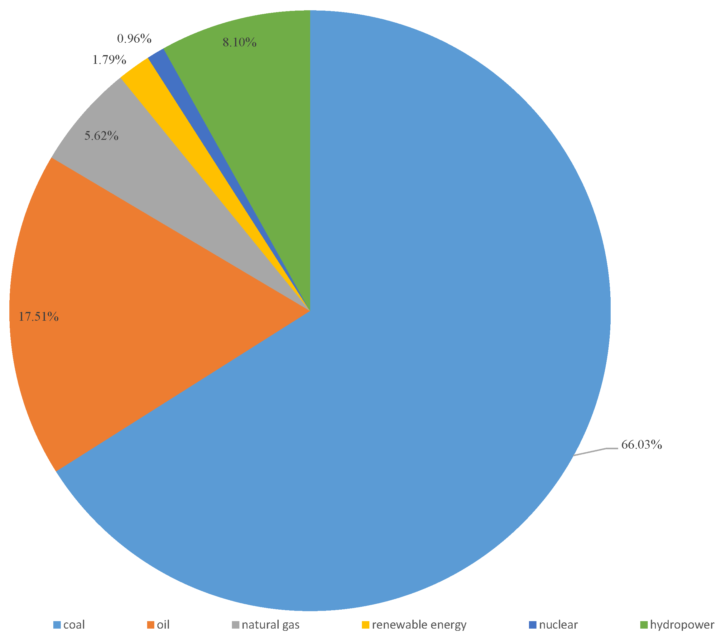
As illustrated in Figure 1, the consumption of coal, oil, and natural gas resource accounted for about 90% of the total energy consumption. Therefore, using the consumption of coal, oil, and natural gas resource to estimate b is reasonable, particularly selecting the proven reserves of coal, oil, and natural gas at the end of 2014 as $h-{\displaystyle {\sum }_{n=1}^x{a}_n}$, and the consumption of coal, oil, and natural gas resources from 1978 to 2014 as ${\displaystyle {\sum }_{n=1}^x{a}_n}$. Accordingly, we computed h as 65.05 billion tons of standard coal. We obtained energy production a in 1978 from the China Statistical Yearbook. Then, using Equation (23), we computed b as 0.0365, which implies that the amount of energy was reduced by 3.65% annually.

5.2. Calculation of the Contribution Rate

The parameters were estimated through the regression analysis and the contribution rate of each factor to agricultural growth rate was calculated. The contribution rates are summarized as follows:

According to

Table 4. Contribution rate of the factor to the agricultural growth rate (%).

π (K)	π (L)	π (T)	π (W)	π (E)
76.86	−1.19	1.08	0.07	1.01

, the contribution rate of labor was negative, which suggests a decline in agricultural labor force. Besides, because the progress of technology was not included in the model, the sum of the five factors’ contribution rates was less than 80%. Therefore, the contribution rate of technological progress was estimated to be about 22.17%.

5.3. Calculation of Trend Forecast of the Growth Drag

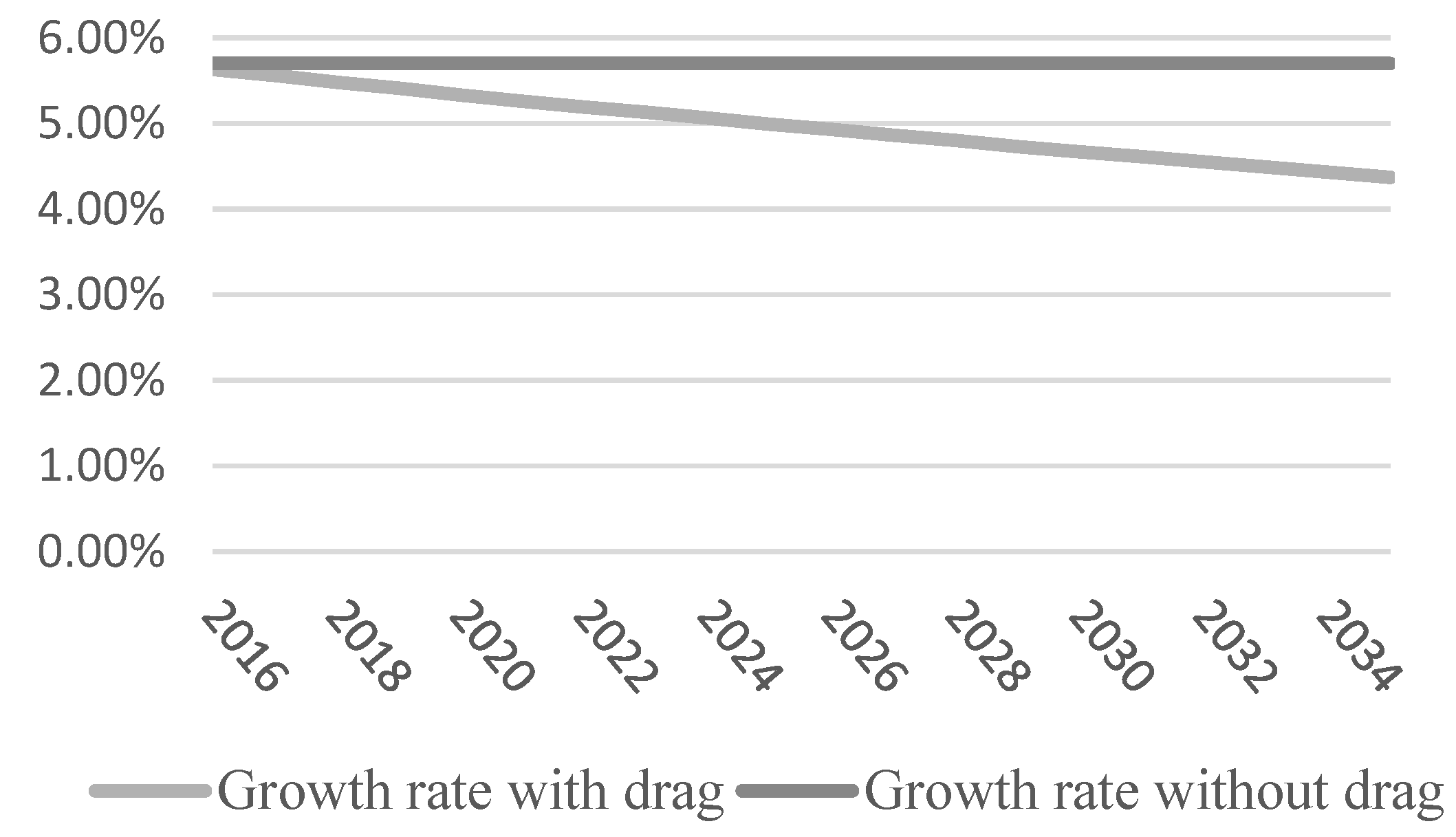
We calculated that the average annual growth rate of agricultural output to be 5.7%. However, due to a growth drag, the annual growth rate of agricultural economy is expected to decline gradually. The real agricultural growth rate can be calculated through Equation (25):

$$\widehat{g_Y}=g_Y(t)\times {(1-Drag)}^{i-2015},i=2016,2017,\dots ,2035$$

(25)

where Drag denotes the sum of the drags of three factors, which is 1.32%. In addition, the annual agricultural growth rate is also calculated. The results are summarized in

Table 5. Real agricultural growth drag under a 5.7% growth rate.

Year	2016	2017	2018	2019	2020	2021	2022	2023	2024	2025
Growth rate	5.625	5.556	5.477	5.405	5.334	5.263	5.194	5.125	5.058	4.991
Year	2026	2027	2028	2029	2030	2031	2032	2033	2034	2035
Growth rate	4.925	4.860	4.796	4.732	4.670	4.608	4.547	4.487	4.428	4.370

.

The real agricultural growth rate decreases as the year evolves, which essentially reflects the effect of growth drag. As Figure 2 shows, due to the influence of the growth drag, growth rate decreases. Hence, the agricultural output in 2035 could be estimated using the output in 2015 as the base line through Equation (26):

$$GD{P}_{2035}=GD{P}_{2015}\prod _{i=2016}^{2035}(1+{\stackrel{\wedge }{g}}_{Y,i}),$$

(26)

where ${\stackrel{\wedge }{g}}_{Y,i}$ denotes the agricultural growth rate of year i. With a growth drag, the agricultural output in 2035 was estimated to be 2.75 times of the output in 2015. If there is no growth drag, the agricultural output in 2035 would be 3.03 times of that in 2015. In essence, based on the growth rate of 5.7%, we found that agricultural output would decrease by 0.28 times in 20 years due to the effect of a growth drag.

6. Discussion

The results show that the drags of land resource, water and energy is 0.0050, 0.0044, and 0.0038, respectively.

Considering the total drag, Xue et al. (2004) [12] computed China’s growth drag of land resource as 0.0175; Xie et al. (2005) [13] computed China’s growth drag of water and land as 0.0146 (i.e., the drag of land is 0.0132 and that of water is 0.0014). The agricultural growth drag is about 90% of China’s growth drag. This drag accounts for a large part of China’s economic growth drag, which reflects a high dependency of the agricultural economy on resource.

Observing the drag of each factor, the agricultural growth drag of water is larger than China’s economic growth drag of water (Xue et al., 2004) [12], which shows a high dependency of the agricultural economy on water. Moreover, the drag of land resources computed in this study is less than that computed by Xie et al. (2005) [16]. All other research results are shown in

Table 6. The Growth drag computed by other scholars.

	Water	Land	Energy	Total Drag
Xue, Wan et al.		0.0175		0.0175
Xie, Wang et al.	0.0014	0.0132		0.0146
Yang, Nie et al. (agriculture)	0.0047	−0.0002		0.0045
Shen, Li			0.0058	0.0058
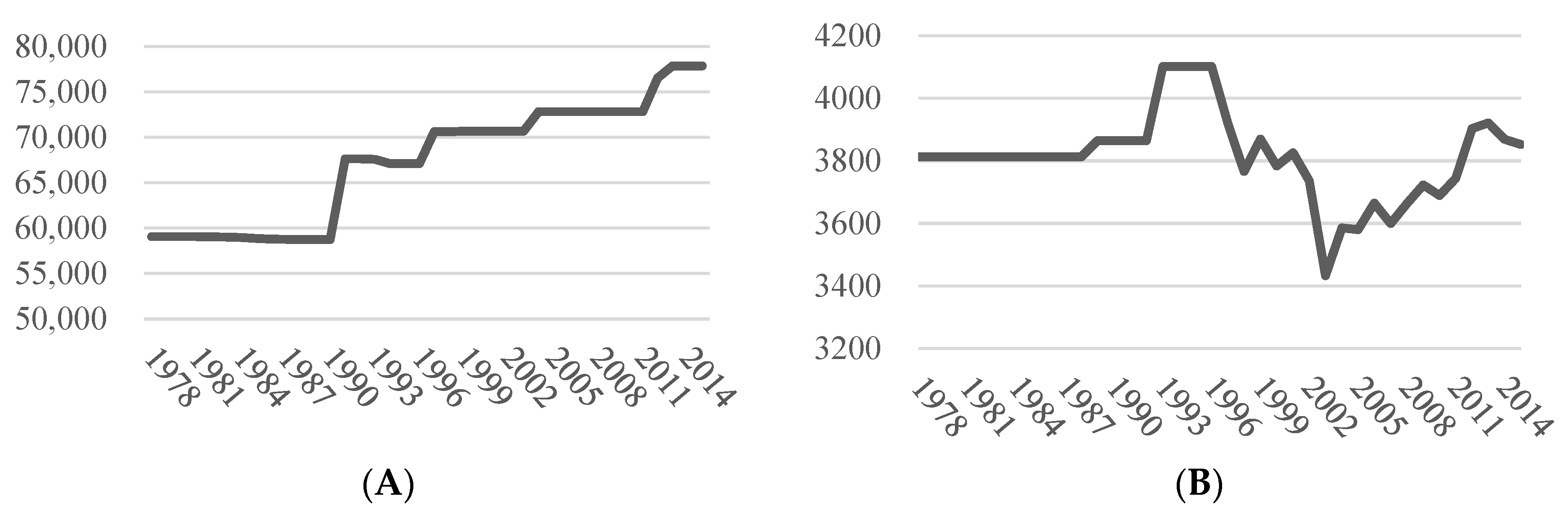
Our study (agriculture)	0.0044	0.0050	0.0038	0.0132

. This is because China’s land resource continues to decrease, and in the long term, agricultural land use has an upward trend (see Figure 3A). Therefore, the calculated value of agricultural growth drag of land is smaller.

The agricultural growth drag of water we calculated is not different from that of Nie et al. (2011)’s estimate [15], but the drag of land is found to be quite different. On the one hand, this paper adds an energy factor to the model, which can cause the decline of drags from other factors. Hence, this may explain why the growth drag of water calculated in our study is slightly smaller than others’ work. On the other hand, the assumptions of our analysis and Yang’s analysis for the growth rate of land and water resources are different, which may explain why the results were also found to be different.

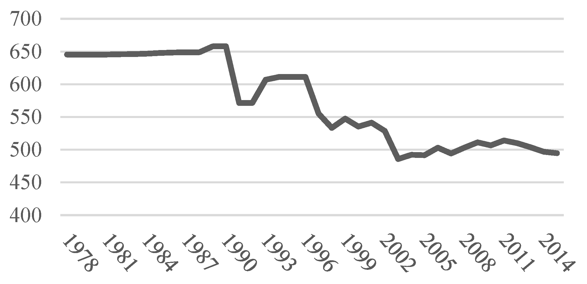
The agricultural growth drag of energy is smaller than that of the water and land resources, and the agricultural growth drag of water and that of the land have a little difference. However, the drag of land is reducing, and that of water is increasing, because agricultural land use is not reducing. As shown in Figure 3B, the agricultural water consumption is decreasing in general. Although this consumption increased after 2004, it can be seen from Figure 4 that the amount of agricultural water consumption and land use decreased. In addition, China’s uneven distribution of water resources, increased industrial water consumption due to industrialization, as well as water supply and demand contradictions, have an impact on the drag of water. In addition, water and land resources have some connection, because soil and water loss and land desertification due to water shortage also has an impact on agricultural production. All of these factors can increase the agricultural growth drag of water.

The agricultural growth drag caused by energy is 0.3799%, which means that the agricultural growth of China reduces by 0.3799% annually, due to the consumption of energy. China’s economic growth drag of energy computed by Shen et al (2010) [22] is 0.577%. Although the impact of energy on agriculture is less than that on China’s overall economy, the agricultural growth drag of energy and that of water and land resources have little difference, so the impact of energy consumption on agriculture cannot be ignored.

There are still some limitations in this paper and some work which is needed in the future: (1) There are many factors influencing the progress of agricultural technology, which have not been analyzed because of the limitation of the paper length and data availability. The drag model does not include technology factors and the total power of agricultural machinery in the regression analysis. However, the technological progress contributes to agricultural economic growth; we know that the growth of agricultural output and agricultural technological progress are closely linked. In the follow-up study, these factors need to be analyzed. (2) Sub-regional studies are needed in the future. Agriculture sectors play an important role in the development of China’s economy. As we all know, there are more than 30 provinces in China, and these provinces are quite different from each other. For example, the north-east of China is the main grain producing area in China, while the Hunan province is the main rice producing area in China. The coast area in China is moist, and the north-west area is quite dry. The agriculture conditions are varied throughout the whole of China, no matter the natural conditions or economic conditions, such as investment or human capital. This is one of the weakness of this paper, as we took these variations as a whole and we did not consider the differences. Therefore, during the future research, the difference between the provinces should be paid more attention. It is quite necessary to interpret the difference policies for different provinces. (3) The relationship between the technology progress and the investment in agriculture should be paid a lot of attention. How much investment should be added to the agriculture to accelerate technological progress also should not be ignored, because it is technological progress that plays a key role in the sustainable development of China’s agriculture. (4) As for the sustainable development of agriculture in China, there are some others factors, such as the mix of crops planted, the civilization, and immigration, and of redundant labor in rural areas, and the lack of sustainable perspectives in rural farmers. This last one may be one of the most important factors. After all, only if rural farmers have sustainable ideas can they implement these idea to the development of agriculture. (5) Moreover, institutional factors are also important for the sustainable development of agriculture, such as security systems. Agriculture is relatively weak compared to the other industries. Therefore, there are many protection systems and subsidy measures for farmers in the developed countries. As developing country, China also should set up a protection system to cover market risks and natural hazards. However, it is difficult to bring institutional factors into the econometric analysis. How to bring institutional factors into the analysis frame is also one of the directions for future research.

7. Conclusions

For a deeper understanding of the effect of land, water, and resources on agricultural economic growth, we carried out an impact assessment of the growth drag of agriculture in China, based on Romer’s growth drag theory. The results show that the total agricultural growth drag caused by water, land, and energy is 1.315%, which suggests that annual agricultural economic growth declines by 1.315% compared to the previous year. Notably, agricultural outputs with a growth drag in 2035 will fall to 72% of that without growth drag, which needs our attention. Besides, the growth drags from land, water, and energy are found to be 0.5%, 0.44%, and 0.38%, respectively. The drag model does not include technology factors and the total power of agricultural machinery in the regression analysis. Thus, we calculate that the contribution rate of technological progress is about 22.17%.

With climate change, urbanization, and the decline of water, land and energy, China is facing increasing challenges. To foster a long-term sustainable agricultural development, considering that the growth drags of agriculture are mainly determined by labor, capital stock output elasticity, and the growth rate of resources, the findings provide the following policy implications: (1) The utilization efficiency of agricultural water resources needs to be improved. Given that the utilization efficiency of agricultural water resources in China is about 80% of that in developed countries, better irrigation scheduling methods are key to increase the efficiency of the irrigation system and enhance agricultural sustainability. (2) New techniques of agricultural energy-saving machinery needs to be adopted so that the energy efficiency could be improved. (3) More supports on innovations and modernization are also essential to achieve a sustainable development in agriculture.