“One Belt, One Road” Initiative to Stimulate Trade in China: A Counter-Factual Analysis

Abstract

This research implements the panel data control method to evaluate the stimulative effects of the “One Belt, One Road” initiative on trade performance in China. We constructed a counterfactual of China’s trade surplus by exploiting the unobservable common factors that create observable trade balances among other countries. We also modified the traditional control group selection by extending it to the Elastic-Net method. This study found the following: (i) China’s annual trade surplus increased sharply by 10.69% on average since 2015. In contrast, analysis of the counterfactual showed that the net exports of China would have remained constant without the stimulation of the “One Belt, One Road” initiative; (ii) These results are robust to exports growth rates and checking by various control group selections; (iii) Although the analysis shows return to an average trading balance, we should not underestimate the benefits of the initiative in the long run.

1. Introduction

China has formulated a new Silk-Road strategy, referred to the “One Belt, One Road” initiative, implemented under the Xi Jinping administration. The move aimed at stimulating growth and improving ties with nations along its geographic periphery. The “One Belt, One Road” initiative (hereafter OBOR) has been viewed as not only a regional development policy, but also a grand strategy to achieve the “Chinese dream”. In this paper, we evaluate the current benefits brought about by OBOR by predicting what would have happened to China’s exports if the initiative had not been implemented. This paper concludes by discussing the effects of OBOR on trade surplus and exports growth rate in the 2015q1–2018q1 period, with comments on export performance drawn from our empirical data analysis.

The OBOR initiative is expected to lead China’s GDP growth, motivated by external demands, greater cooperation in Asia, strengthening of institutions, and a deeper integration throughout Asia-Europe-Pacific. In the study period, China’s real growth rate slowed down to around 7%—more than four percent points from its fastest-growing period. China has been attracting investments and initiating wider policies in order to bring its growth rate back on track [1]. The country has aroused national attention to the questions: (i) Can the OBOR initiative promote a new moderate trading balance. (ii) Are nations located in the OBOR region forming economic ties for mutual well-being? (iii) Has the initiative been welcomed by most countries worldwide?

Answering these questions involves estimating the effects of this new policy on current Chinese trades efforts, which, however, face several difficulties. First, it is impossible to show trading balances in a scenario where the initiative has not been implemented. Second, it is not easy to model how and why the trading balance of a country fluctuated over time, as well as identify the factors that have driven these changes.

To answer the above queries, we adopted a method proposed by Hsiao et al. [2] (hereafter HCW) to construct a counterfactual of China. As trade surplus of countries is often driven by common factors, trends in other economic zones can be used to predict the total trading values in China over time. Therefore, using the trading performance of countries that not subject to OBOR partners, we estimate what would happen to China if the initiative hadn’t been implemented, and also reflect on the country’s efforts to maintain a high level of trade.

In addition, a subtle problem lies is the optimal selection of control countries to synthesize a counterfactual of China. As most countries are not major trading partners with China, we choose remote countries as control candidates. Moreover, as a large number of countries would lower the predictivity ability of the model, choosing the right ones was a difficult task. We, thus, engaged the Elastic-Net method proposed by Zou et al. [3] to resolve the issue. In a $K\ge N$ variables selection case, the Elastic-Net method performed better than other similar methods (such as Lasso) [3].

With the help of a proper control group, our results showed that the trade surplus of China from 2015 to 2018 would have remained at an average level of US$ 170 million quarterly, had there been no trade promotion. In other words, China’s policy of greater openness increased the average trading balance of the country by 10%. A robustness check also examined the exports growth rate of China and found that its performance remains satisfactory in this era of shrinking global markets, thus supporting the main findings of this study.

Therefore, based on our empirical analysis, our answers to the overheating trade debates are: (i) The OBOR initiative has a significant effect on trade promotion; (ii) The yearly trade surplus of China doubled to US$ 130 billion on average after three quarters of implementation effort; (iii) The OBOR initiative offers the opportunity to intensively tie up with the rest of the world, leading to future prosperity.

1.1. Literature Review

There have been several studies conducted on the impacts of openness on economic growth. Grossman and Helpman [4] believed that free trade based on comparative advantages could enable participators to specialize in the creation of knowledge and production of goods that make intensive use of human capital and new technologies. Edwards et al. [5] encouraged developing countries to open wide their doors to initiate industrialization and narrowing of the gap with rich countries. Nannicini et al. [6] proved that trade liberalization could lead to economic growth by adopting the synthetic control method that estimates the counter-factual situation of a country in the absence of regime change. They tested the impacts of openness on most developing countries, and verified that there is a positive effect of openness on average. Madsen [7] proposed that trade influences economic growth though knowledge and importing of high-quality intermediate goods; the empirical test conducted showed that the Total Factors of Production was positively related to the trade liberalization in 16 industrialized countries. For developing countries, Sarkar et al. [8] drew an unpropitious conclusion on trade openness; they showed an insignificant relation between free-trade and growth in the case of North Korea and India. Ju et al. [9] found strong and consistent evidence that trade liberalization leads to higher imports and exports, in contrast to Santos-paulino et al. [10], who found a robust negative impact of trade liberalization on the net trade balance. Berggren et al. [11] showed that a positive effect of free trade on economic growth is not robust if one uses the Least Trimmed Squares-based estimation to reach a conclusion. Focusing on the Chinese economy, Arnold [12] pointed out: “It is conceivable that the US-Sino relationship is indispensable to its continued prosperity.” Most recently, Lu et al. [13] examined data after China’s WTO accession, and revealed that trade liberalization reduces makeup dispersion in a narrowly defined industry.

In this study, we conducted empirical analysis with reference to Hsiao et al. [2]. However, Du et al. [14] evaluated home-purchase restrictions in China using a counter-factual analysis; they modified the method proposed by Hsiao et al. [2] by using the leave-n_v-out cross-validation criterion as an optimal choice for the control units. Ouyang et al. [15] applied a semi-parametric model and Hsiao et al.’s method [2] to investigate the macroeconomic effects of the 2008 Economic Stimulus Program in China; the treatment effect depended on the difference between the actual and counter factual values. Abadie et al. [16] applied the synthetic control method, which is similar to the HCW approach, to appraise Proposition 99 in California. They synthesized a California as the convex weighted combination of other states that without implementing the statute by key predictors for cigarette consumption. Unlike Hsiao et al.’s approach [2], the matching dimensions were chosen by the authors’ subjective judgment rather than factor-loading estimations [16]. Similarly, Abadie et al. [17] exercised this technique and constructed the Basque Country without terrorism by weighing a combination of nearby economies. The weighted elements are macroeconomic variables in this case. In another counter-factual analysis study, Billmeier et al. [18] also adopted the synthetic control approach to apprise trade-liberalization effects for developing countries in Asia and Africa, which parallelly endorses our study. Bove et al. [19] proved that there is a similarity between panel and synthetic control estimations in an empirical study. Munasib et al. [20] used the synthetic control method to establish a baseline projection for revealing economic shocks brought about by soaring energy prices.

This paper contributes by evaluating the outcome of the OBOR to trading performances in China and proposing a better model selection criterion to select control units for synthesizing a counter-factual China without policy intervention. Our study provides empirical evidence for evaluation of the OBOR initiative, which may further assist policy reforms in China.

1.2. Institutional Background

According to Chinese National Statistics, China’s real growth rate has been slowing down to 6–7% since year 2015, which implies that China is currently in a transitional period, shifting from a double-digit rate of growth to a much slower growth. The Xi Jinping administration proposes the “new normal” slogan, which primarily aims at a stable economic growth while making the structure reformed, instead of pursuing a high growth rate. China is seeking new opportunities for trade and economic integration with towards the west and the south by adopting the OBOR initiative [21]. In late 2013 (September–October), Chairman Xi announced the idea of building a Silk Road Economic Belt and a 21st Century Maritime Silk Road, which jointly make up the OBOR concept [21]. By widening to the world internal introduction and external linkage, OBOR is expected to promote economic structural changes, transformations, and industrial upgradation in China [22].

This strategy entails developing infrastructure, creating a large economic market by strengthening relations between China and various nations in Central Asia, Europe, Middle East, North Africa and Southeast Asia, and easing excess production capacity by exporting, thereby promoting its economic growth rate [23]. China has been actively involved with regional trade organizations worldwide since the end of the last century [23]. OBOR can, thus, be simply seen as a new name for the consolidation of efforts that China has already made in economic ties with Asia, Europe, and the Arab World [23]. However, the OBOR differs from China’s previous foreign policy in two ways: first, the opening up offers a larger geographic scope by turning the western interior into the frontier; second, the OBOR involves opening up to the east and west and efforts on land and sea [1]. Indeed, the OBOR is presented as an essential element of Beijing’s attempt to deepen economic reform within China and stimulate development in China’s western regions.

Although China has put huge efforts into the OBOR, there are several obstacles. Beijing is allocating huge amounts of finance to the project via the Asia Infrastructure Investment Bank, but China’s neighbors remain wary of OBOR’s geopolitical implications [21]. Many observers believe that China might eventually use the initiative to establish unwelcome spheres of influence or dominance over its neighbors [23]. A large portion of the regions covered by OBOR has an unstable security and political situation; in reality, progress on the economic corridors has slowed. Many countries located in the OBOR region are exceedingly poor with limited ability to trade and undertake huge infrastructures, and have considerable levels of corruption. Obviously, there is an apparent complimentary between the needs of countries surrounding China and China’s huge financial resources and extensive experience in undertaking infrastructure projects. This, therefore, needs a serious examination to understand how such an endeavor could be undertaken and completed in a profitable and genuinely beneficial manner [21]. OBOR has only just started, but there are several uncertainties on the specifics of its progression and it had not gone the way China planned [1].

Convincing the world that the OBOR is a good opportunity and winning over popular sentiment will be important keys for its success. There will be calls for domestic reforms in China, and the OBOR initiative will be put to the test. Despite various perspectives on the OBOR, this paper only focuses on the OBOR’s stimulation effects on trade in China.

2. Research Model

This section illustrates the HCW method and Elastic-Net control units’ selection procedures to analyze the treatment effects of the OBOR.

2.1. The HCW’s Factor Model Approach

Hsiao et al. [2] propose a factor model approach to estimate a policy intervention effect by using panel data. Li and Bell [24] confirm that by using the HCW method, one can consistently estimate the average treatment effect, and the result is robust to any nonlinear functional form. Meanwhile, Bai et al. [25] confirm that the HCW method provides consistent results for non-stationary data, which certifies that HCW is a valuable tool for macroeconomic policy evaluations. This section will first introduce their notation and assumptions, and combine the methodology with our research target.

By focusing on trade balances across countries, the panel data ${\left\{Y_{it}\right\}}_{i=1,t=1}^{N,T}$ represents information across countries in recent years. Let $Y_{it}^0$ and $Y_{it}^1$ denote a country i’s trading balances before the policy intervention occurs in period t and after the treatment, respectively. ${\Delta }_{it}=Y_{it}^1-Y_{it}^0$ captures the treatment effect of macroeconomic policy to the i th country at time t, which is not observable. HCW [2] finds other units that are not subject to intervention and relies on the correlations among cross-section units to predict what would have happened to the i th unit had it not been subject to policy intervention. The HCW [2] method realized treatment effect evaluation by constructing the counter-factual of the missing outcome $y_{it}^0$.

Following Hsiao et al. [2], we assume that there exist common factors $f_t$ that drive trading performance of all countries over time. These factors can be GDP growth rate, technology and innovations, etc. Therefore, we have the following factor model:

$$Y_{it}^0=b_{it}^{\prime }{f}_t+{\alpha }_i+{\epsilon }_{it},i=1,\dots ,N,T=1,\dots ,T,$$

(1)

where $b_i$ denotes the $K\times 1$ vector of factor loading for country i, ${\alpha }_i$ is the fixed country-specific effect, and ${\epsilon }_{it}$ is the idiosyncratic error term with $E\left({\epsilon }_{it}\right)$ = 0. Stacking $N\times 1$ $y_{it}^0$ into a vector yields:

$$y_{it}^0=B{f}_t+\alpha +{\epsilon }_t$$

(2)

where $y_t^0=(y_{1t}^0,\dots ,y_{it}^0)\prime$, $\alpha =（{\alpha }_1,\dots ,{\alpha }_N）\prime$, ${\epsilon }_t=({\epsilon }_{it},\dots ,{\epsilon }_{Nt})\prime$, and $\mathrm{B}=(b_1,\dots ,b_N)\prime$ is the $N\times K$ factor loading matrix.

Let $Y_{it}^1$ denote trading balances of China at time t under the OBOR initiative. The observable data usually are:

$$y_{it}=d_{it}{y}_{it}^1+(1-d_{it})y_{it}^0$$

(3)

where $d_{it}=1$ of country i is within the OBOR region at time t, and $d_{it}=0$ otherwise.

At time $T_1+1$, here September 2013, as greater trade openness used to play a part with a time lag, we decide $T_1+1$ is the first year after year 2014. Therefore:

$$Y_{1t}=Y_{1t}^1\hspace{1em}t=T_1+1,\dots ,T.$$

(4)

For countries that have not taken part in the Chinese initiative, we have:

$$Y_{it}=Y_{it}^0\hspace{1em}i=2,\dots ,N,t=1,\dots ,T.$$

(5)

The estimated effect of the “One Belt, One Road” initiative in China at time t will be:

$${\Delta }_{it}=Y_{1t}^1-Y_{1t}^0$$

(6)

Both N and T are large in our data; we can predict the counter-factual $Y_{1t}^0,t=T_1+1,\dots ,T.$ by adopting the HCW [1] method, which also requires the following assumptions:

Assumption A1.

$\left\{{\epsilon }_t\right\}$is a stationary and ergodic process with$E\left[{\epsilon }_t\right]=0,E=\left[{\epsilon }_t{f}_t^{\prime }\right]=0$and$E\left[{\epsilon }_t{\epsilon }_t^{\prime }\right]=V$, where V is a diagonal constant matrix.

Assumption A2.

Rank(B) = K.

Assumption A1 is standard in the literature. Assumption A2 implies that the number of observable cross-sectional units, N, is greater than the number of common time-varying factors $f_t$. With two assumptions and Equation (1), HCW [2] derives that:

$$y_{1t}^0=\overline{\alpha }+a_{-1}^{\prime }{y}_{-1t}+{\epsilon }_{1t}^{\ast }$$

(7)

where henceforth

$$y_{-1t}=(y_{2t},\dots ,y_{Nt})\prime ,$$

(8)

$\overline{\alpha }$ and $a_{-1}$ are constants, and ${\epsilon }_{1t}^{\ast }$ is some error term uncorrelated with $y_{-1t}$.

Equation (7) suggests using $y_{-1t}$ in lieu of $f_t$ to predict $y_{1t}^0$. One problem is choosing the control countries $y_{-1t}$; it is not optimal to include all other countries. Instead of using the Akaike information criterion (AIC, Akaike) [26,27] or the corrected Akaike information criterion (AICC, Hurvich and Tsai) [28] for selection of control countries, we modify the HCW procedure [2] by using the Elastic-Net method.

2.2. Control Variable Selection by Elastic-Net

We modified the HCW control group selection procedure [2] by using Zou and Hastie’s method [3]. Our empirical analysis showed that the Elastic-Net encourages a grouping effect, which could result in the inclusion of too many control candidates and a multi-correlation problem; therefore, we removed countries that are highly correlated in our OLS regression (

Table 1. Control groups selection: weights of control groups (2003q1–2013q4).

Columbia	3.829	Georgia	−62.651	Israel	7.701
	(0.46)		(−1.60)		(1.30)
UK	−0.434	Holland	1.120	Bolivia	−13.586
	(−0.91)		(0.42)		(−0.84)
Romania	−4.055	Ecuador	−12.681 *	Czech Republic	−9.067
	(−0.58)		(−1.91)		(−1.73)
Swiss	−0.081	Nigeria	−0.248	Iceland	−55.579 *
	(−0.04)		(−0.41)		(−2.09)
Egypt	−8.956 **	Finland	2.419	Bulgaria	8.828
	(−2.44)		(0.55)		(0.96)
Romania	−4.055	Chile	1.774	Sweden	3.177
	(−0.58)		(0.69)		(0.75)
Swiss	−0.081	Egypt	−8.956 **	Ivory Coast	11.379
	(−0.04)		(−2.44)		(1.49)
Austria	−7.988	France	−0.229
	(−1.46)		(−0.18)
Intercept	−36.761
	(−1.18)
T      44
F(36,7)	22.71
r2	0.9915
Adj_r2	0.9478

t statistics in parentheses; Significance levels: *: p < 0.1; **: p < 0.05; ***: p < 0.01.

).

The variable selection method becomes increasingly important in modern data analysis, when the number of predictors is large [3]. Ridge regression aims to improve prediction and interpretation of OLS by minimizing the residual sum of squares subject to a bound on the $L_2-norm$ of the coefficients; however, it cannot produce a parsimonious model, for it always keeps all predictors in the model [29]. Penalization techniques have been improved based on the shrinkage method; the most promising is Lasso, proposed by Tibshirani [30], wherein both continuous shrinkage and automatic variable selection occurs simultaneously by imposing an $L_1$ penalty on the regression coefficients. Although Lasso has succeeded in many aspects, it has limitations. Take, for example, these two scenarios: (a) When $K>N$, Lasso selects most variables before it saturates, because of the nature of the convex optimization problem; (b) Lasso tends to select only one variable from a group that has high pairwise correlations, and lacks the ability to reveal the grouping information [31]. Both scenarios make Lasso less appropriate in variable selections.

Zou and Hastie [3] propose a variable selection method—Elastic-Net—which has outperformed Lasso in a simulation study. Zou et al.’s Elastic-Net [3] method often derives a more satisfactory result than Lasso, especially in $K\ge N$ variable selection cases. As $K\ge N$ and grouped variables situations are common, Elastic-Net often outperforms Lasso in terms of prediction accuracy by amending over-shrink and group information revelation problems [30]. Zou et al. [3] use the penalized least square method for shrinkage:

$$\widehat{\beta }=\arg \underset{\beta }{\min }{\left|y-X\beta \right|}^2,\mathrm{subject}\mathrm{to}\left(1-\alpha \right){\left|\beta \right|}_1+\alpha {\left|\beta \right|}^2\le t\mathrm{for}\mathrm{some}t.$$

(9)

Zou and Hastie [3] propose $\left(1-\alpha \right){\left|\beta \right|}_1+\alpha {\left|\beta \right|}^2$ as the Elastic-Net penalty in Equation (9), which is a convex combination of the Lasso and Ridge penalty. For $\alpha \in$[0, 1), the Elastic-Net penalty function is singular (without the first derivative) at 0 and is strictly convex for all $\alpha >0$, thus offering the characteristics of both Lasso and Ridge regression; $\alpha =0.5$ represents a typical Elastic-Net [3].

Zou and Hastie [3] employ the 10-fold cross-validation (CV) method to estimate prediction error and compare different models by choosing tuning parameters; a grid value of ${\lambda }_2$ is given, and the other tuning parameter is selected by tenfold CV. Estimated ${\lambda }_2$ is the one that gives the smallest CV error.

We may combine Elastic-Net with the HCW method [2] to synthesize a counter-factual China in the following empirical study.

3. The Treatment Effects of the OBOR Initiative in China

This section aims to produce quantitative estimates of the influence of the OBOR initiative on China’s key macroeconomic variable—trade balances by using HCW [2] panel data approach for program evaluation. Firstly, we estimate the correlations between the trade surplus of China and those of the control countries using the pre-treatment data. We then apply the estimates to construct post-treatment counterfactuals for China. The difference between the predicted counterfactuals and the actual observed trade surplus will be the estimated stimulation effects of the OBOR.

3.1. Data

Data of trading performance across countries are from the UN Comtrade and China Economic statistical databases. The national custom services in each trading country provides data on monthly imports, exports, and trading growth rates up to 40 years. We picked seasonal adjusted trading balances in US$ and exports’ growth across countries in the last 15 years for variable observation. In addition, by testing the existence of unit roots in all data series, we augmented the Dickey-Fuller test results for candidate countries. China shows stationarity in data series trading performance (see Figure 1 and Figure 2).

3.2. Control Group Selection and Treatment Effects Estimation

We synthesized a counter-factual China to uncover a hypothetical outcome in the absence of interventions to the “One Belt, One Road” initiative. Nations that display strong correlations should share common latent factors; we, thus, apply Equation (1) to estimate the correlations between the treatment and control nations based on pre-treatment data.

In selection of control economies, we looked for those that not only share common factors with the Chinese economy, but are also relatively independent of the OBOR in the post-treatment period 2014q1–2018q1. More specifically, to examine the trade relationships between China and potential control economies and to satisfy the assumption of policy intervention exogenesis to the control group [15]. Common time-varying factors $f_t$, individual specific effects ${\alpha }_i$ and a random component ${\epsilon }_{it}$ drive trade balances varying over time in Equation (1). We assume that idiosyncratic components ${\alpha }_i$ and${\epsilon }_{it}$ are uncorrelated across countries. Lasso2 package in Stata/MP 13.1, developed by Ahrens et al. in early 2018, was used. Lasso2 package is a program for Lasso, Square-Root Lasso, Elastic-Net, Ridge, Adaptive Lasso and Post-estimation Ordinary Least Square (available at http://ideas.repec.org/c/boc/bocode/s458458.html).

Countries such as Australia and New Zealand do not hesitate in participating in Chinese initiatives, which are also welcomed by China’s Asian neighbors. We, thus, exclude these participants and the neighboring countries as control units, to avoid treatment contamination. Applying the Elastic-Net method, the machinery learning selection results identify the select countries: Columbia, UK, Romania, Swiss, Egypt, Austria, Ecuador, Nigeria, Finland, Chile, Israel, Bolivia, Czech Republic, Iceland, Bulgaria, Sweden, Georgia, Holland, Lebanon, Tunisia, Jordan, Peru, Malta, Azerbaijan, Hungary, Sri Lanka, India, Luxembourg, Russia, Uruguay, Turkey, Estonia, Norway, Portugal and France, which is consistent with our illustrated artificial selection criteria.

In another counter-factual analysis study, Billmeier et al. [18] adopted the synthetic control approach to describe the trade-liberalization effects. They included Asian countries such as India, Pakistan, Nepal, Philippines, Bangladesh, Nepal, China; African countries such as Morocco, Nigeria, Rwanda, South Africa, Ivory Coast, Cameroon, Uruguay, Zambia, Zimbabwe, Egypt, Tunisia; and Latin American countries such as Argentina, Colombia, Costa Rica, Chile, Paraguay, Peru and Brazil in the control group to synthesize developed Asian countries such as South Korea, Japan, and Singapore. Unlike their selection criteria, our control group is majorly composed of East European countries. Focusing on our research objective and also taking reality into account, Asian countries near China that have active trading partnerships were removed from the control group. Meanwhile, the rational of selecting a control group is to keep them clear of policy contamination, and thus it is best to choose remote countries to synthesize a counter-factual China.

The trade surplus of China appears to be well approximated by the chosen controls before treatment. Our real data analysis below (Figure 1) confirms this point. The control group produces a counter-factual path that closely traces the actual path of China before the implementation of the OBOR initiative with a ${\overline{R}}^2$ of 0.9478. The OLS estimated weights are listed in Table 1, the estimated counterfactuals of China before the policy intervention are listed in

Table 2. Counterfactuals for China before treatment (US$ billion).

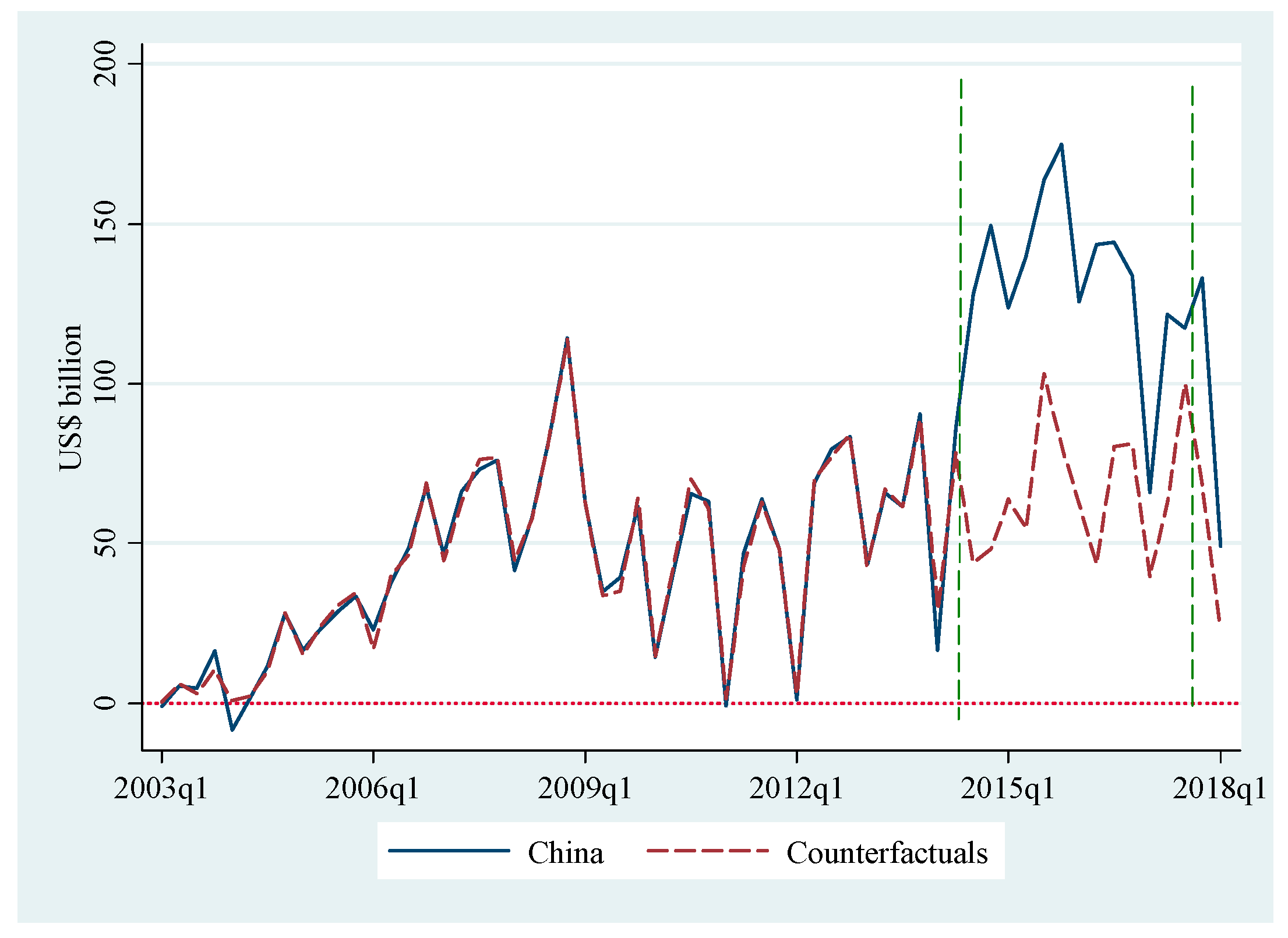
Time	China	Counterfactuals
2003q4	16	10
2004q4	28	28
2005q4	34	34
2006q4	68	69
2007q4	76	77
2008q4	114	114
2009q4	62	64
2010q4	63	61
2011q4	48	48
2012q4	83	84
2013q4	91	89

Data source: CEIC China Statistical database.

; we have only listed statistics of the last quarter in each year for counterfactuals before treatment (Table 2).

The counterfactuals of China, constructed on the control group after the OBOR initiative was implemented, are reported in

Table 3. Counterfactuals for China after treatment (US$ billion).

Time	China	Counterfactual	Treatment
2014q1	17	29	−12
2014q2	86	79	7.3
2014q3	128	44	84
2014q4	149	48	101
2015q1	124	64	60
2015q2	140	55	85
2015q3	164	103	60
2015q4	175	81	94
2016q1	126	62	63
2016q2	143	44	100
2016q3	144	80	64
2016q4	134	81	53
2017q1	66	39	27
2017q2	122	63	59
2017q3	117	100	17
2017q4	133	68	65
2018q1	49	23	26

Data source: CEIC China Statistical database.

; the estimated quarterly treatment effects are simply the difference of the actuals and the counterfactuals. Statistics summary of treatment effects listed in Table 3 are highly positive. The pre- and post-intervention actual and predicted outcomes with a significant gap are plotted in Figure 1.

In Figure 1, the hypothetical line tracks the solid line quite closely before treatment, suggesting a good fit by estimation settings. Starting from the treatment quarter, the hypothetical line separates from the actual line: actual growth moves above the hypothetical counterfactual trade balance, implying that there is positive treatment effect.

Four years after the initiative was announced, the actual trade surplus averaged at 130 billion US$; the estimated counterfactual trade surplus of China in the absence of the OBOR is about 60 billion US$ quarterly, on average. The treatment effect of the initiative would be valued as doubling Chinese net exports.

Several remarks should be made regarding the timing of the treatment effects. The hypothetical line moves close to the solid line and tracks it closely again towards the end of 2017 (on the right side of the second dashed vertical line), suggesting that the treatment effect is getting weaker due to the recent trade war. Our estimates suggest that, in the absence of this enormous trade promotion, net exports could be cut in half with President Trump initiating the US-Sino trade war in 2017. Although trade surplus showed a declining trend in the beginning of 2018, there is no reason to believe that the influence of the OBOR economic integration cannot last in the long-run. Greater openness could have a profound influence on this developing country.

3.3. Robustness Check

This section evaluates the effects of OBOR on China’s exports growth rate. For a robustness check, we continue to use the same control group and experimental period, and then construct counterfactuals again to investigate treatment effects.

We use seasonal adjusted quarterly export growth rates of the selected control countries to construct a counterfactual for China in the absence of the OBOR initiative. Using the same procedure described in Section 3.2, we first obtain OLS weights based on statistics for the period of 2005: q1–2014: q1 listed in

Table 4. Weights of control groups: 2003q1–2013q4.

Luxemburg	−0.105	Uruguay	−0.302	Ecuador	−0.552
	(−0.54)		(−1.66)		(−1.95)
Bolivia	0.571 **	Finland	0.457	Romania	−0.492
	(2.62)		(1.57)		(−1.47)
Austria	2.322 ***	Azerbaijan	0.026	Turkey	0.530 **
	(4.81)		(1.94)		(2.73)
Hungary	0.449	Swiss	−0.192	Georgia	0.126 *
	(1.70)		(−1.23)		(2.38)
Jordan	−0.148	Bulgaria	−0.734 **	India	0.061
	(−0.60)		(−2.91)		(0.26)
Lebanon	−0.050	Nigeria	0.242 **	France	−2.127
	(−0.71)		(2.74)		(−1.16)
Chile	0.357 *	Malta	0.177	Estonia	−0.320 *
	(2.31)		(1.39)		(−2.56)
Iceland	−0.142	Russia	0.202	Peru	0.360
	(−1.39)		(0.85)		(1.86)
Egypt	−0.396 ***	Sri Lanka	0.066	UK	0.695 **
	(−4.60)		(0.39)		(3.47)
Tunisia	0.174	Norway	0.171	Portugal	−1.303 **
	(0.63)		(0.73)		(−3.79)
Intercept	7.401
	(1.25)
T	36
F(30,5)	46.24
r2	0.996
Adj_r2	0.9749

t statistics in parentheses; significance levels: *: p < 0.1; **: p < 0.05; ***: p < 0.01.

. The counterfactual path produced by the control groups is confirmed in Figure 2; it closely traces the actual path of China’s export growth rates before the implementation of OBOR with a ${\overline{R}}^2$ of 0.996.

In

Table 5. Counterfactuals for China before treatment.

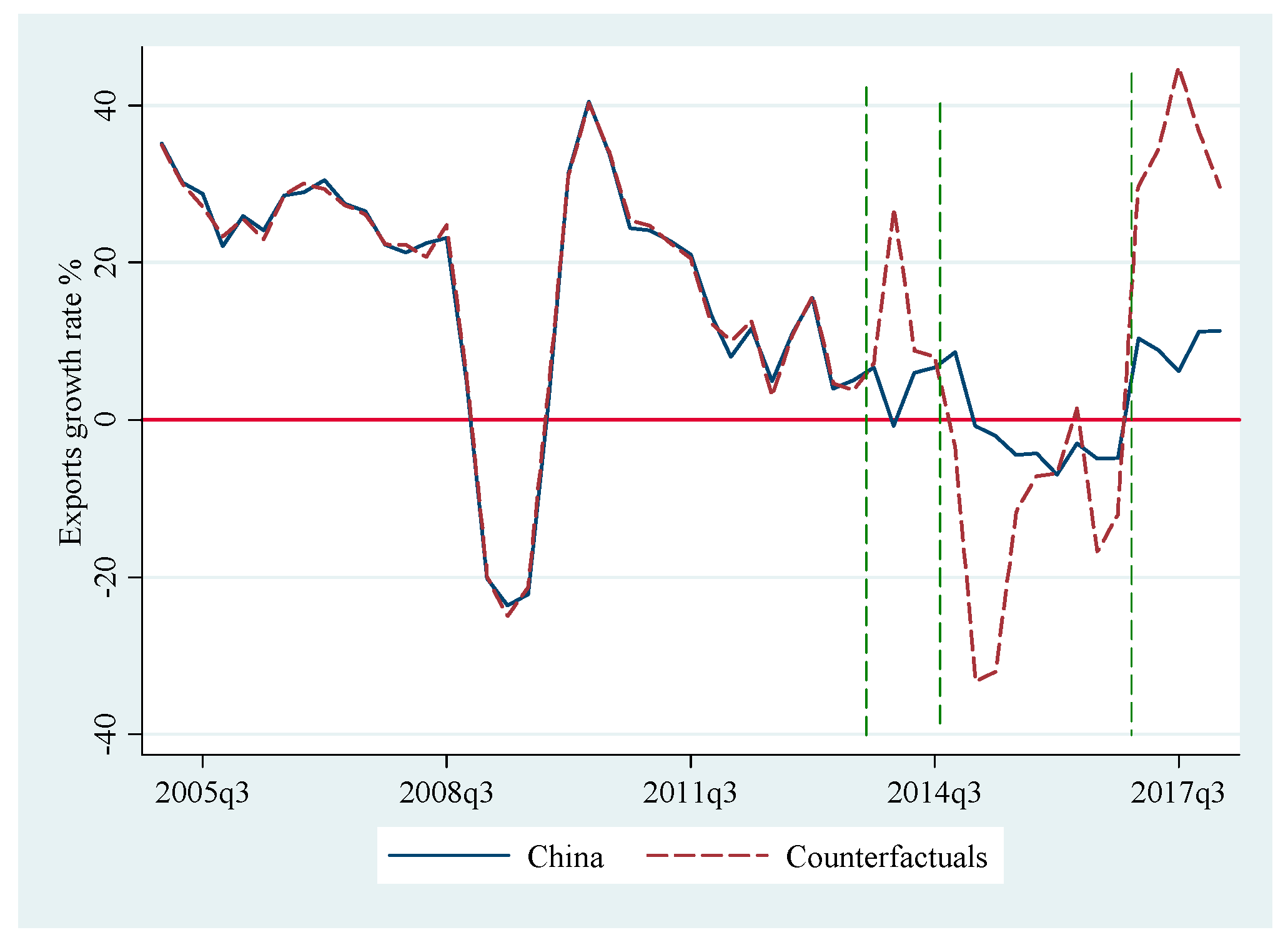
Time	China	Counterfactual
2005q4	22	23.34
2006q4	29	30.05
2007q4	22	22.32
2008q4	4.7	5.37
2009q4	2.2	3.63
2010q4	24	25.39
2011q4	13	12.28
2012q4	11	10.82
2013q4	6.7	7.16

Data source: CEIC China Statistical database.

, the difference between actual growth rates and synthesized counterfactuals are below 1percent point on average; therefore, errors within a small range can be tolerated. Figure 2 shows that the hypothetical line follows the solid line quite closely before treatment, suggesting a good fit by estimation settings. The actual and estimated counterfactual exports growth rate in the absence of the “One Belt, One Road” initiative has been about 12% yearly on an average, after the Global Financial Crisis of 2008.

The robustness checking result supports the fact that the OBOR significantly increased China’s exports during the observed period. The estimated average treatment effect on exports growth rate from 2014:q1 to 2018:q1 is 8 percent points (

Table 6. Counterfactuals for China after treatment.

Time	China	Counterfactual	Treatment
2014q1	−0.73	26.95	−27
2014q2	6	8.81	−3.4
2014q3	6.6	8.11	−0.66
2014q4	8.6	−3.40	20
2015q1	−0.73	−33.26	42
2015q2	−2.1	−32.04	46
2015q3	−4.5	−11.81	19
2015q4	−4.3	−7.12	13
2016q1	−7	−6.87	8.3
2016q2	−3	1.43	−2.3
2016q3	−4.9	−16.73	16
2016q4	−4.9	−12.14	13
2017q1	10	29.76	−25
2017q2	8.9	34.40	−23
2017q3	6.2	44.88	−35
2017q4	11	36.62	−27
2018q1	11	29.66	−20

Data source: CEIC China Statistical database.

), and is significant at the 1% level according to the asymptotic distribution derived by Li et al. [24]. Specifically, in the background of global trade shrinkage, the average actual exports growth rate remains positive, while the average predicted exports growth rate without extra trade promotions is much likely to be below zero points. The estimated treatment effects indicate that the exports growth rate has been boosted by more than 8 percent points, compared to the growth rate had there been no initiative.

Figure 2 shows that, starting from the treatment quarter until the middle of 2014, between the first vertical line and the second vertical line, the hypothetical line separates from the actual line with an unstable trend, implying a testing treatment period (we are not certain when the OBOR initiative began to be effective). Subsequently, the observation period between the second vertical line and the third vertical line in Figure 2 shows a certain positive treatment effect on exports growth from 2014 to 2016.

Owing to the OBOR initiative, China’s exports growth rates did not drop as sharply as the global trend, which is extraordinary given the country’s enormous trade quantities. Treatment effects were estimated to be negative after 2016 (the facts are presented in Section 3.2). Although China has shown a slower exports growth rate than other developing economies since 2016 (after the third dash vertical line in Figure 2), primarily caused by the US-Sino trade war, it now shows a small positive rate of around 7 percent points owing to stimulation by the OBOR initiative.

We also collected data of China’s exports from the Organization for Economic Co-operation and Development (OECD) and plotted an increasing trend in market share (Figure 3), which is another evidence of the effectiveness of the “One Belt, One Road” scheme. There is a slight peak in market share for the period of 2014 to 2016 (after the second dash line); it shows the stimulation of the scheme on total exports in China. The time-series of China’s world market share provide obvious evidence of the short-run effectiveness of the “One Belt, One Road” initiative.

4. Conclusions

The OBOR program was implemented in early 2013, and is considered as one of the most significant initiatives ever proposed worldwide. In this paper, we try to assess the impact of the economic integration of the “One Belt, One Road” region on China’s economy by comparing what actually happened to China’s trades with what would have happened if the initiative had not been implemented. More specifically, we wish to analyze how the initiative has changed the trading performance of China.

While the post-treatment outcome is affected by many time-varying latent factors, there are difficulties in evaluating the real effects of policy interventions. The approach by Hsiao et al. [2] offers more flexibility by allowing the influence of common latent factors to vary across section, which makes the method more applicable to reality. The HCW method helps us construct counterfactuals of the missing outcomes, which allows us to predict what would have happened to the i th unit had it not been subject to the policy intervention.

Applying both HCW [2] framework and Elastic-Net for semi-parametric settings enables the manipulation of the dependence of trade surplus in countries without much connection to China in order to construct a counterfactual China. We estimate that the OBOR initiative increased trade surplus by about 50–60%, but with a descending trend. The stimulative effects of OBOR on trade is also evident in the estimation of other economic indicators, such as net exports growth rate. However, the most recent US-Sino trade war initiated by President Trump has had a negative impact on Chinese trading performance. We derive that, in the absence of the OBOR trade promotion, the net exports growth rate from 2017 would have shown a decline.

With little share in domestic consumption, the Chinese economy depends heavily on investments and net exports, and seeks to initiate a large trading program worldwide. The OBOR initiative could also become an important component of China’s reform and development in the long term.

References

- Aoyama, R. “One Belt, One Road”: Chin’s New Global Strategy. J. Contemp. East Asia Stud. 2016, 5, 3–22. [Google Scholar] [CrossRef]
- Hsiao, C.; Ching, H.S.; Wan, S.K. A Panel Data Approach for Program Evaluation: Measuring the Benefits of Political and Economic Integration of Hongkong with Mainland China. J. Appl. Econom. 2012, 27, 705–740. [Google Scholar] [CrossRef]
- Zou, H.; Hastie, T. Regularization and Variable Selection via the Elastic Net. J. R. Stat. Soc. Ser. B Stat. Methodol. 2005, 67, 301–320. [Google Scholar] [CrossRef]
- Grossman, G.M.; Helpman, E. Trade, Innovation, and Growth. Am. Econ. Rev. 1990, 80, 86–91. [Google Scholar]
- Edwards, S. Openness, Trade Liberalization, and Growth in Developing Countries. J. Econ. Lit. 1993, 31, 1358–1393. [Google Scholar]
- Nannicini, T.; Billmeier, A. Economies in Transition: How Important Is Trade Openness for Growth? Oxf. Bull. Econ. Stat. 2011, 73, 287–314. [Google Scholar] [CrossRef]
- Madsen, J.B. Trade Barriers, Openness, and Economic Growth. South. Econ. J. 2009, 76, 397–418. [Google Scholar] [CrossRef]
- Sarkar, P. Trade Openness and Growth: Is There Any Link? J. Econ. Issues 2008, 42, 763–785. [Google Scholar] [CrossRef]
- Ju, J.; Wu, Y.I.; Zeng, L.I. The Impact of Trade Liberalization on the Trade Balance in Developing Countries. IMF Staff Pap. 2010, 57, 427–449. [Google Scholar] [CrossRef]
- Santos-Paulino, A.; Thirlwall, A.P. The impact of trade liberalisation on exports, imports and the balance of payments of developing countries. Econ. J. 2004, 114, F50–F72. [Google Scholar] [CrossRef]
- Berggren, N.; Jordahl, H. Does Free Trade Really Reduce Growth? Further Testing Using the Economic Freedom Index. Public Choice 2005, 122, 99–114. [Google Scholar] [CrossRef]
- Kashia, A. Alexander Del Mar: Free Trade and the Chinese Question. South. Calif. Q. 2012, 94, 304–345. [Google Scholar]
- Lu, Y.; Yu, L. Trade Liberalization and Markup Dispersion: Evidence from China’s WTO Accession. Am. Econ. J. Appl. Econ. 2015, 7, 221–253. [Google Scholar] [CrossRef]
- Du, Z.; Zhang, L. Home-purchase restriction, property tax and housing price in China: A counterfactual analysis. J. Econom. 2015, 188, 558–568. [Google Scholar] [CrossRef]
- Ouyang, M.; Peng, Y. The treatment-effect estimation: A case study of the 2008 economic stimulus package of China. J. Econom. 2015, 188, 545–557. [Google Scholar] [CrossRef]
- Abadie, A.; Diamond, A.; Hainmueller, J. Synthetic Control Methods for Comparative Case Studies: Estimating the Effect of California’s Tobacco Control Program. J. Am. Stat. Assoc. 2010, 105, 493–505. [Google Scholar] [CrossRef]
- Abadie, A.; Gardeazabal, J. The Economic Costs of Conflict: A Case Study of the Basque Country. Am. Econ. Rev. 2003, 93, 113–132. [Google Scholar] [CrossRef]
- Billmeier, A.; Nannicini, T. Assessing Economic Liberalization Episodes: A Synthetic Control Approach. Rev. Econ. Stat. 2013, 95, 983–1001. [Google Scholar] [CrossRef]
- Bove, V.; Eliay, L.; Smith, R.P. The Relationship between Panel and Synthetic Control Estimators of the Effect of Civil War; BCAM Working Paper 1406; Birkbeck Centre for Applied Macroeconomics: London, UK, 2014. [Google Scholar]
- Munasib, A.; Rickman, D. Regional economic impacts of the shale gas and tight oil boom: A synthetic control analysis. Reg. Sci. Urban Econ. 2015, 50, 1–17. [Google Scholar] [CrossRef]
- Dollar, D. China’s rise as a regional and global power. J. Int. Relat. Sustain. Dev. 2015, 1, 12–14. [Google Scholar]
- Swaine, M.D. Chinese Views and Commentary on the “One Belt, One Road” Initiative. China Leadersh. Monit. 2015, 2, 3. [Google Scholar]
- Nalbantoglu, C. One Belt One Road Initiative: New Route on China’s Change of Course to Growth. Open J. Soc. Sci. 2017, 5, 87–99. [Google Scholar] [CrossRef]
- Li, K.T.; Bell, D.R. Estimation of average treatment effects with panel data: Asymptotic theory and implementation. J. Econom. 2017, 197, 65–75. [Google Scholar] [CrossRef]
- Bai, J. Inferential Theory for Factor Models of Large Dimensions. Econometrica 2010, 71, 135–171. [Google Scholar] [CrossRef]
- Akaike, H. A new look at the statistical model identification. IEEE Trans. Autom. Control 1974, 19, 716–723. [Google Scholar] [CrossRef]
- Akaike, H. Factor analysis and AIC. Psychometrika 1987, 52, 317–332. [Google Scholar] [CrossRef]
- Hurvich, C.M.; Tsai, C. Regression and time series model selection in small samples. Biometrika 1989, 76, 297–307. [Google Scholar] [CrossRef]
- Hoerl, A.E.; Kennard, R.W. Ridge Regression: Biased Estimation for Nonorthogonal Problems. Technometrics 2000, 42, 80–86. [Google Scholar] [CrossRef]
- Zou, H.; Zhang, H.H. On the Adaptive Elastic-Net with a diverging number of Parameters. Ann. Stat. 2009, 37, 1733–1751. [Google Scholar] [CrossRef] [PubMed]
- Tibshirani, R. Regression shrinkage and selection via the lasso: A retrospective. J. R. Stat. Soc. Ser. B Stat. Methodol. 2011, 73, 273–282. [Google Scholar] [CrossRef]