Using Information on Settlement Patterns to Improve the Spatial Distribution of Population in Coastal Impact Assessments


Abstract
1. Introduction
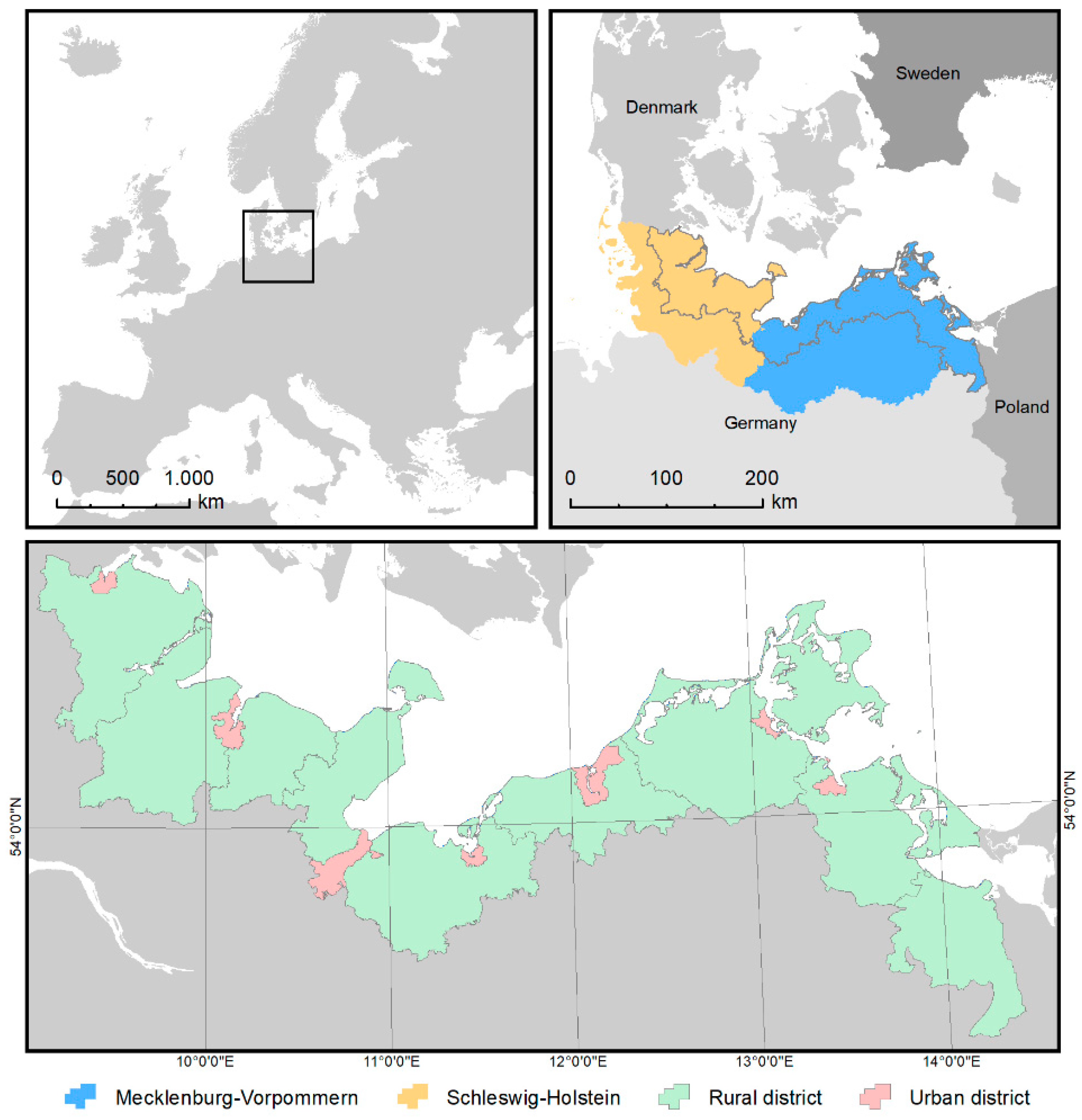
2. Study Area
3. Data and Methods.
3.1. Data
3.1.1. Population
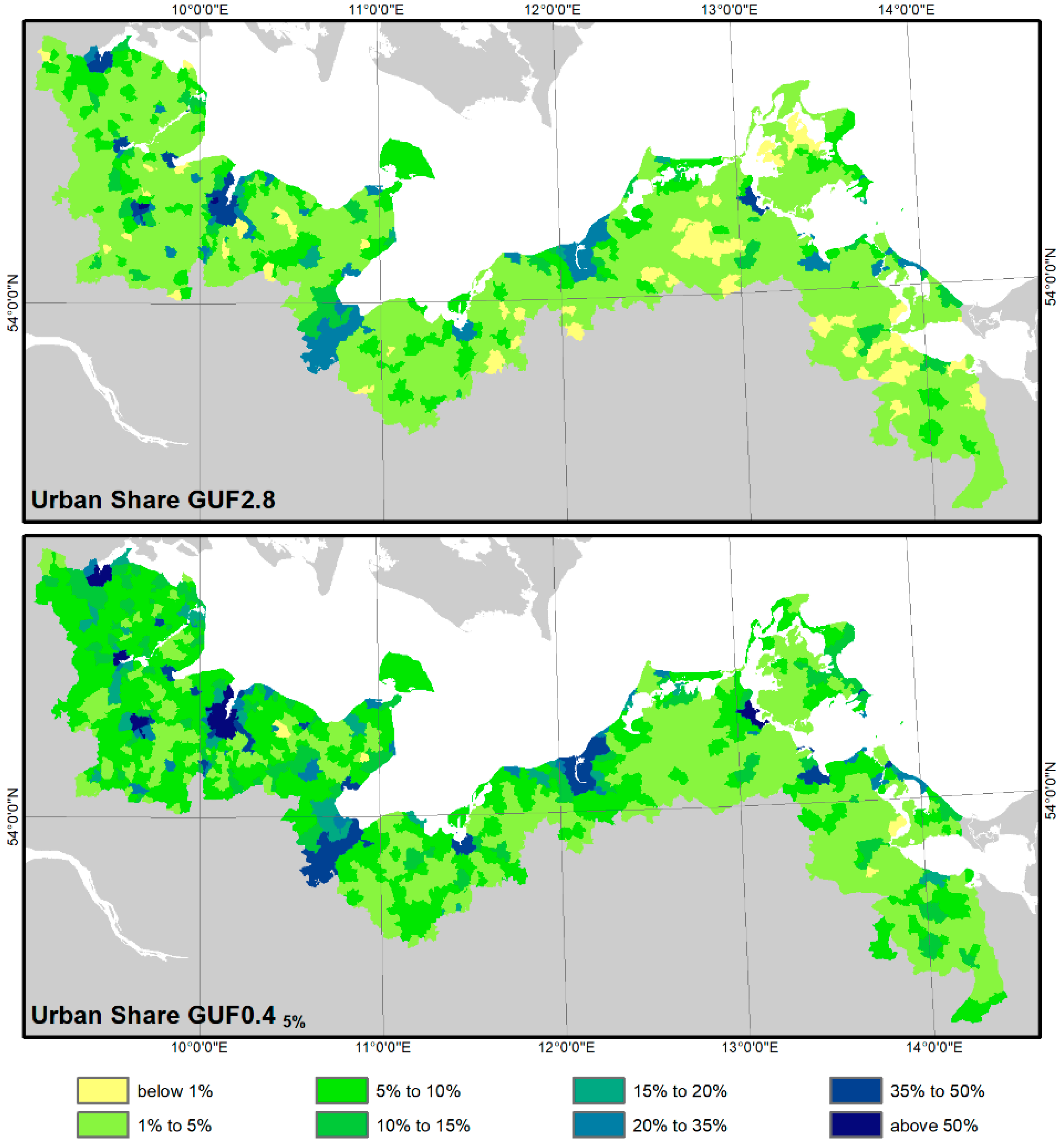
3.1.2. Urban Extent
3.1.3. Exposed Area
3.2. Resampling of Population
4. Results and Discussion
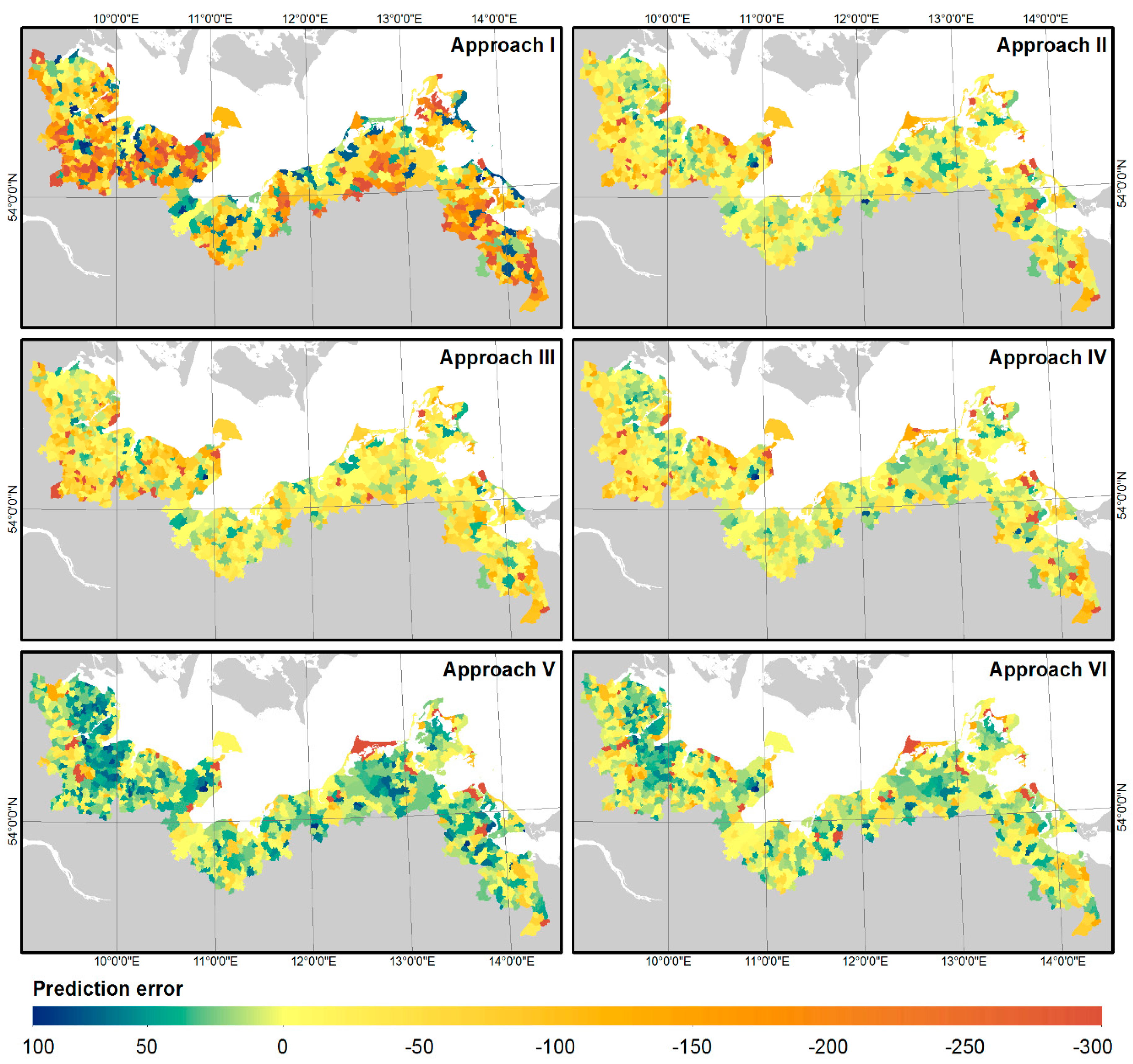
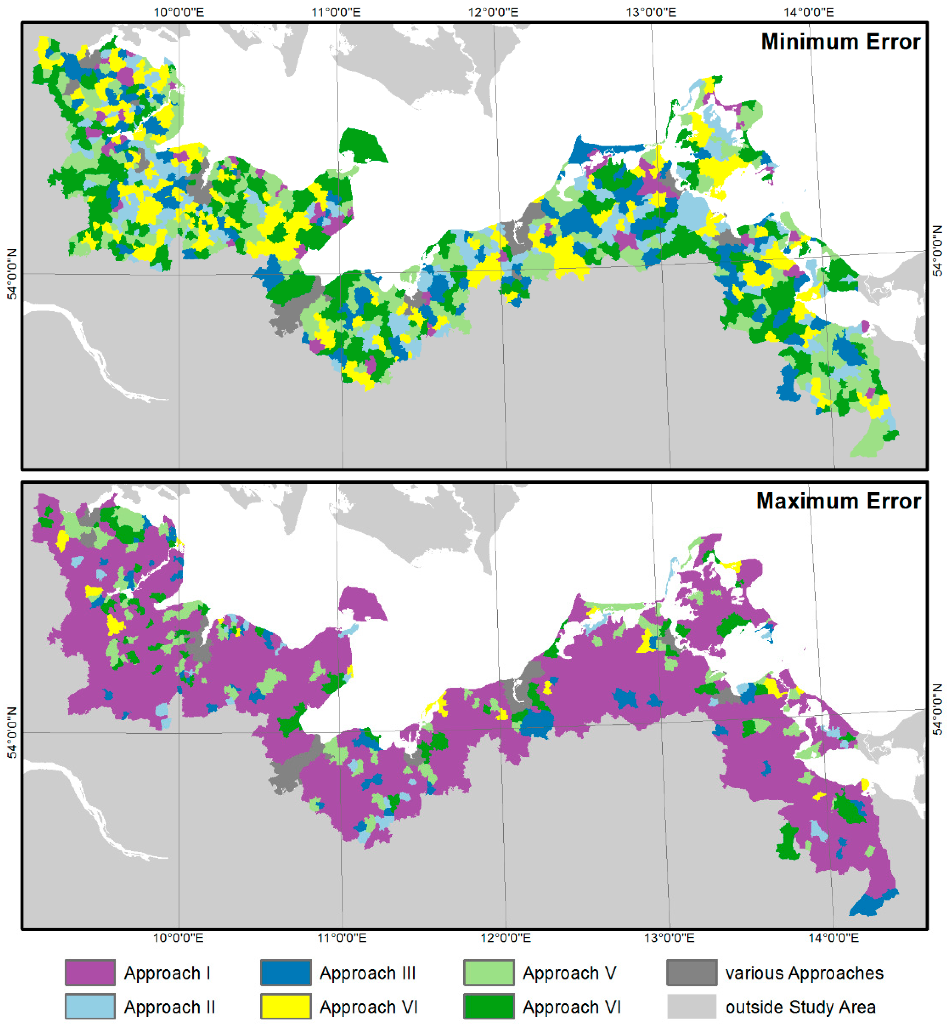
4.1. Performance on Municipality Level
4.2. Exposed Population
5. Conclusions
Author Contributions
Funding
Acknowledgments
Conflicts of Interest
Appendix
Model Description
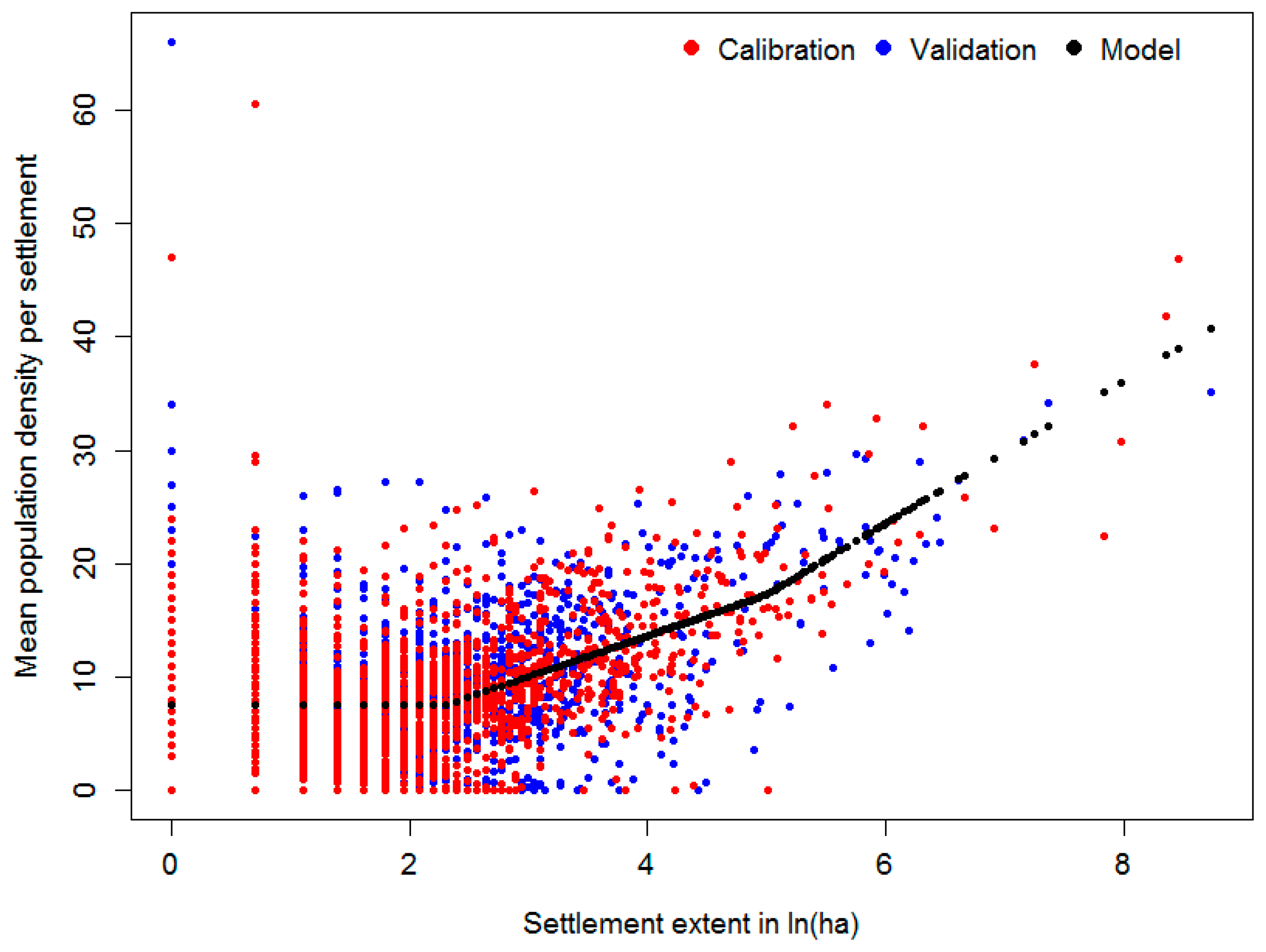
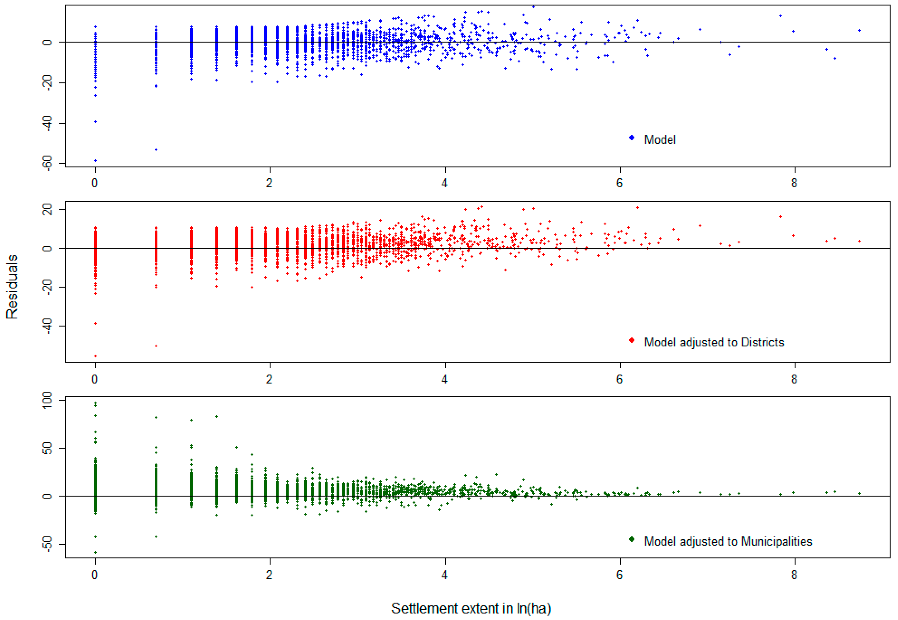
Approach V

| Parameter | Calibration Mean Density | Validation Mean Density | Calibration Population Sum | Validation Population Sum |
|---|---|---|---|---|
| RMSE | 5.6 | 5.7 | 1007 | 854 |
| MAE | 4.7 | 4.7 | 84 | 96 |

| Parameter | Calibration Mean Density | Validation Mean Density | Calibration Population Sum | Validation Population Sum |
|---|---|---|---|---|
| RMSE (d 1) | 6.6 | 6.4 | 1025 | 682 |
| MAE (d 1) | 5.7 | 5.3 | 95 | 101 |
| RMSE (m 2) | 11.1 | 10.7 | 537 | 419 |
| MAE (m 2) | 9.1 | 7.9 | 85 | 90 |

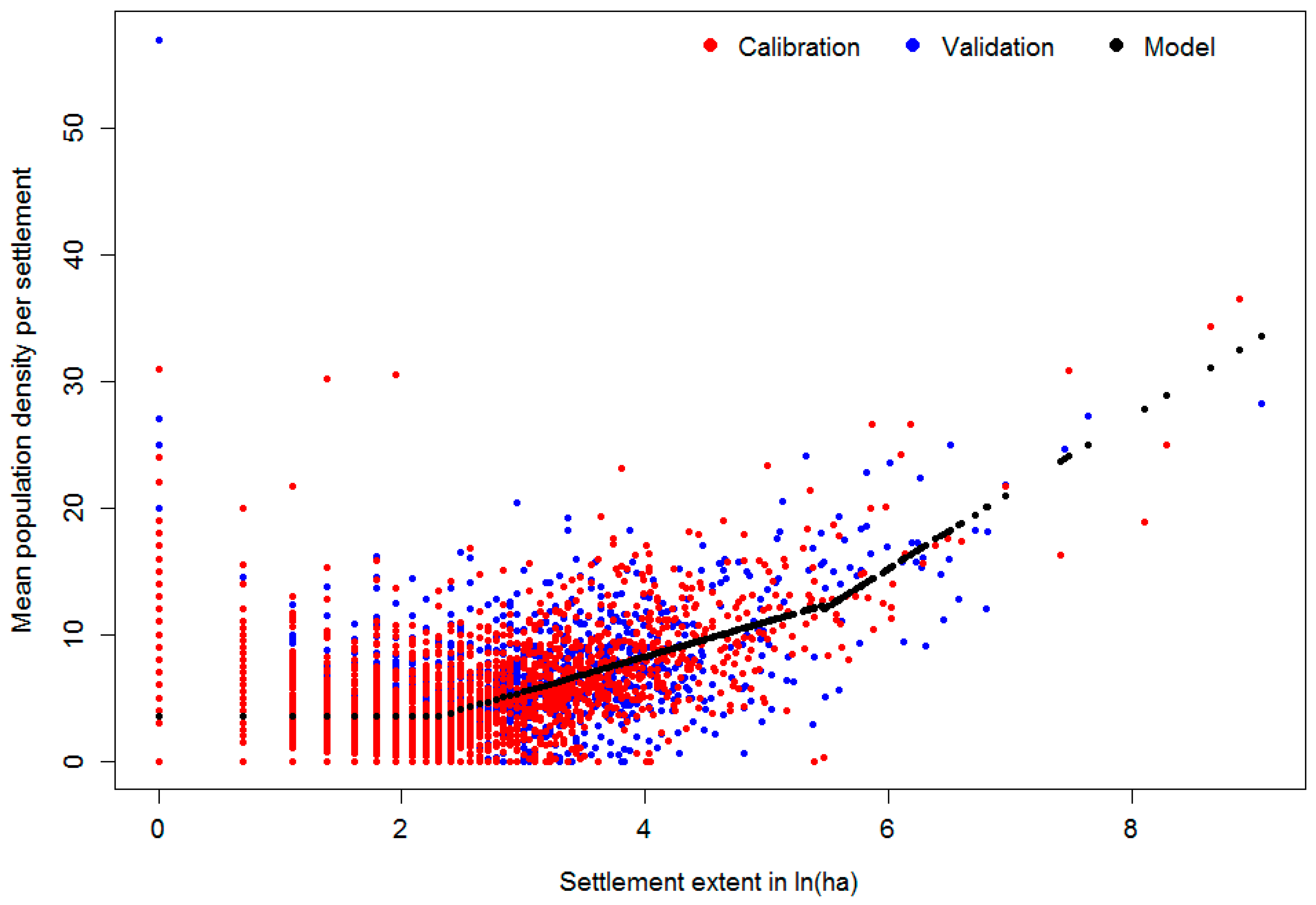
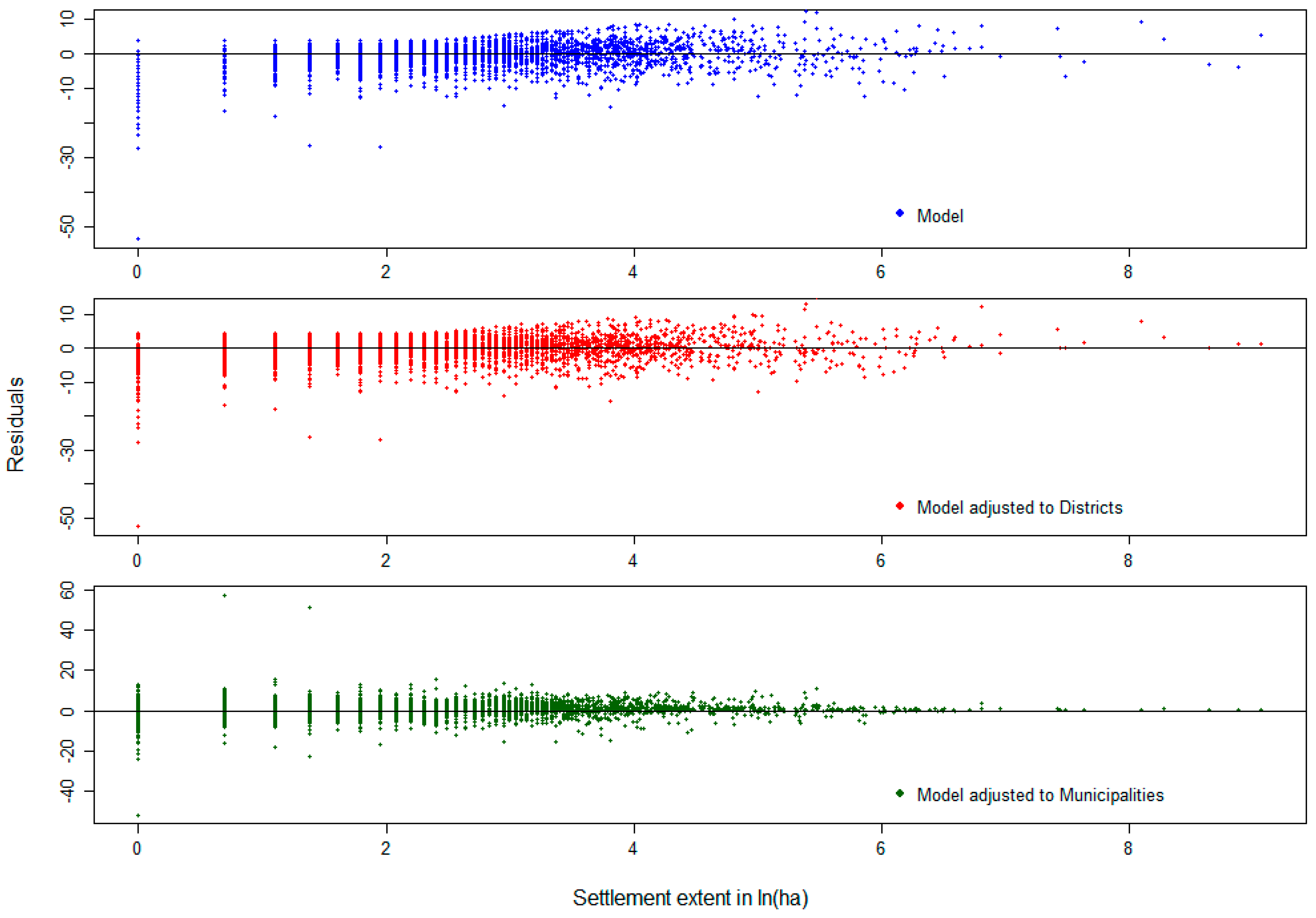
Approach VI
| Parameter | Calibration Mean Density | Validation Mean Density | Calibration Population Sum | Validation Population Sum |
|---|---|---|---|---|
| RMSE | 3.2 | 3.6 | 918 | 1077 |
| MAE | 2.4 | 2.6 | 87 | 107 |

| Parameter | Calibration Mean Density | Validation Mean Density | Calibration Population Sum | Validation Population Sum |
|---|---|---|---|---|
| RMSE (d 1) | 3.2 | 3.6 | 611 | 447 |
| MAE (d 1) | 2.5 | 2.7 | 71 | 86 |
| RMSE (m 2) | 3.5 | 4.2 | 171 | 198 |
| MAE (m 2) | 2.7 | 2.9 | 43 | 55 |

References
- Kron, W. Coasts: The high-risk areas of the world. Nat. Hazards 2013, 66, 1363–1382. [Google Scholar] [CrossRef]
- Nicholls, R.J.; Cazenave, A. Sea-level rise and its impact on coastal zones. Science 2010, 328, 1517–1520. [Google Scholar] [CrossRef] [PubMed]
- Wong, P.P.; Losada, I.J.; Gattuso, J.-P.; Hinkel, J.; Khattabi, A.; McInnes, K.L.; Saito, Y.; Sallenger, A. Coastal systems and low-lying areas. In Climate Change 2014: Impacts, Adaptation, and Vulnerability: Part A: Global and Sectoral Aspects. Contribution of Working Group II to the Fifth Assessment Report of the Intergovernmental Panel on Climate Change; Field, C.B., Barros, V.R., Dokken, D.J., Mach, K.J., Mastrandrea, M.D., Bilir, T.E., Chatterjee, M., Ebi, K.L., Estrada, Y.O., Genova, R.C., et al., Eds.; Cambridge University Press: Cambridge, UK, 2014; pp. 361–409. [Google Scholar]
- Hinkel, J.; Lincke, D.; Vafeidis, A.T.; Perrette, M.; Nicholls, R.J.; Tol, R.S.J.; Marzeion, B.; Fettweis, X.; Ionescu, C.; Levermann, A. Coastal flood damage and adaptation costs under 21st century sea-level rise. Proc. Natl. Acad. Sci. USA 2014, 111, 3292–3297. [Google Scholar] [CrossRef] [PubMed]
- Neumann, B.; Vafeidis, A.T.; Zimmermann, J.; Nicholls, R.J. Future coastal population growth and exposure to sea-level rise and coastal flooding—A global assessment. PLoS ONE 2015, 10, e0118571. [Google Scholar] [CrossRef] [PubMed]
- Merkens, J.-L.; Reimann, L.; Hinkel, J.; Vafeidis, A.T. Gridded population projections for the coastal zone under the Shared Socioeconomic Pathways. Glob. Planet. Chang. 2016, 145, 57–66. [Google Scholar] [CrossRef]
- Jones, B.; O’Neill, B.C. Spatially explicit global population scenarios consistent with the Shared Socioeconomic Pathways. Environ. Res. Lett. 2016, 11, 084003. [Google Scholar] [CrossRef]
- Brown, S.; Nicholls, R.J.; Woodroffe, C.D.; Hanson, S.; Hinkel, J.; Kebede, A.S.; Neumann, B.; Vafeidis, A.T. Sea-Level Rise Impacts and Responses: A Global Perspective. In Coastal Hazards; Finkl, C.W., Ed.; Springer: Dordrecht, The Netherlands, 2013; pp. 117–149. [Google Scholar]
- Neumann, B.; Ott, K.; Kenchington, R. Strong sustainability in coastal areas: A conceptual interpretation of SDG 14. Sustain. Sci. 2017, 12, 1019–1035. [Google Scholar] [CrossRef] [PubMed]
- Vousdoukas, M.I.; Voukouvalas, E.; Mentaschi, L.; Dottori, F.; Giardino, A.; Bouziotas, D.; Bianchi, A.; Salamon, P.; Feyen, L. Developments in large-scale coastal flood hazard mapping. Nat. Hazards Earth Syst. Sci. 2016, 16, 1841–1853. [Google Scholar] [CrossRef]
- Crowell, M.; Coulton, K.; Johnson, C.; Westcott, J.; Bellomo, D.; Edelman, S.; Hirsch, E. An Estimate of the U.S. Population Living in 100-Year Coastal Flood Hazard Areas. J. Coast. Res. 2010, 262, 201–211. [Google Scholar] [CrossRef]
- Hallegatte, S.; Green, C.; Nicholls, R.J.; Corfee-Morlot, J. Future flood losses in major coastal cities. Nat. Clim. Chang. 2013, 3, 802–806. [Google Scholar] [CrossRef]
- Center for International Earth Science Information Network—Columbia University (CIESIN). Gridded Population of the World, Version 4 (GPWv4): Population Density, Revision 10; NASA Socioeconomic Data and Applications Center (SEDAC): Palisades, NY, USA, 2017.
- Center for International Earth Science Information Network—Columbia University (CIESIN); International Food Policy Research Institute (IFPRI); The World Bank; Centro Internacional de Agricultura Tropical (CIAT). Global Rural-Urban Mapping Project, Version 1 (GRUMPv1): Population Count Grid; NASA Socioeconomic Data and Applications Center (SEDAC): Palisades, NY, USA, 2015.
- Paprotny, D.; Morales-Nápoles, O.; Jonkman, S.N. HANZE: A pan-European database of exposure to natural hazards and damaging historical floods since 1870. Earth Syst. Sci. Data 2018, 10, 565–581. [Google Scholar] [CrossRef]
- Reimann, L.; Merkens, J.-L.; Vafeidis, A.T. Regionalized Shared Socioeconomic Pathways: Narratives and spatial population projections for the Mediterranean coastal zone. Reg. Environ. Chang. 2018, 18, 235–245. [Google Scholar] [CrossRef]
- McGranahan, G.; Balk, D.; Anderson, B. The rising tide: Assessing the risks of climate change and human settlements in low elevation coastal zones. Environ. Urban. 2007, 19, 17–37. [Google Scholar] [CrossRef]
- Doxsey-Whitfield, E.; MacManus, K.; Adamo, S.B.; Pistolesi, L.; Squires, J.; Borkovska, O.; Baptista, S.R. Taking Advantage of the Improved Availability of Census Data: A First Look at the Gridded Population of the World, Version 4. Pap. Appl. Geogr. 2015, 1, 226–234. [Google Scholar] [CrossRef]
- Balk, D.L.; Deichmann, U.; Yetman, G.; Pozzi, F.; Hay, S.I.; Nelson, A. Determining Global Population Distribution: Methods, Applications and Data. In Global Mapping of Infectious Diseases: Methods, Examples and Emerging Applications; Meltzer, M.I., Ed.; Elsevier: New York City, NY, USA, 2006; pp. 119–156. [Google Scholar]
- Deville, P.; Linard, C.; Martin, S.; Gilbert, M.; Stevens, F.R.; Gaughan, A.E.; Blondel, V.D.; Tatem, A.J. Dynamic population mapping using mobile phone data. Proc. Natl. Acad. Sci. USA 2014, 111, 15888–15893. [Google Scholar] [CrossRef] [PubMed]
- Sorichetta, A.; Hornby, G.M.; Stevens, F.R.; Gaughan, A.E.; Linard, C.; Tatem, A.J. High-resolution gridded population datasets for Latin America and the Caribbean in 2010, 2015, and 2020. Sci. Data 2015, 2, 150045. [Google Scholar] [CrossRef] [PubMed]
- Gaughan, A.E.; Stevens, F.R.; Linard, C.; Jia, P.; Tatem, A.J. High resolution population distribution maps for Southeast Asia in 2010 and 2015. PLoS ONE 2013, 8, e55882. [Google Scholar] [CrossRef] [PubMed]
- Linard, C.; Gilbert, M.; Snow, R.W.; Noor, A.M.; Tatem, A.J. Population distribution, settlement patterns and accessibility across Africa in 2010. PLoS ONE 2012, 7, e31743. [Google Scholar] [CrossRef] [PubMed]
- Stevens, F.R.; Gaughan, A.E.; Linard, C.; Tatem, A.J. Disaggregating census data for population mapping using random forests with remotely-sensed and ancillary data. PLoS ONE 2015, 10, e0107042. [Google Scholar] [CrossRef] [PubMed]
- Vousdoukas, M.I.; Mentaschi, L.; Voukouvalas, E.; Bianchi, A.; Dottori, F.; Feyen, L. Climatic and socioeconomic controls of future coastal flood risk in Europe. Nat. Clim. Chang. 2018, 3, 802. [Google Scholar] [CrossRef]
- Esch, T.; Schenk, A.; Ullmann, T.; Thiel, M.; Roth, A.; Dech, S. Characterization of Land Cover Types in TerraSAR-X Images by Combined Analysis of Speckle Statistics and Intensity Information. IEEE Trans. Geosci. Remote Sens. 2011, 49, 1911–1925. [Google Scholar] [CrossRef]
- Esch, T.; Heldens, W.; Hirner, A.; Keil, M.; Marconcini, M.; Roth, A.; Zeidler, J.; Dech, S.; Strano, E. Breaking new ground in mapping human settlements from space—The Global Urban Footprint. ISPRS J. Photogramm. Remote Sens. 2017, 134, 30–42. [Google Scholar] [CrossRef]
- Federal Statistical Office of Germany, 2011 Census. Census Database of the Census 2011. Available online: https://ergebnisse.zensus2011.de/?locale=en (accessed on 4 June 2018).
- Ministry of Agriculture and the Environment Mecklenburg-Vorpommern (MLUV-MV). Regelwerk Küstenschutz Mecklenburg-Vorpommern: Übersichtsherft. Grundlagen, Grundsätze, Standortbestimmung und Ausblick; Ministry of Agriculture and the Environment Mecklenburg-Vorpommern (MLUV-MV): Schwerin, Germany, 2009. (In German)
- Sterr, H. Assessment of Vulnerability and Adaptation to Sea-Level Rise for the Coastal Zone of Germany. J. Coast. Res. 2008, 242, 380–393. [Google Scholar] [CrossRef]
- Ministry of Energy, Agriculture, the Environment, Nature and Digitalization Schleswig-Holstein (MELUND-SH). Generalplan Küstenschutz des Landes Schleswig-Holstein: Fortschreibung 2012; Ministry of Energy, Agriculture, the Environment, Nature and Digitalization Schleswig-Holstein (MELUND-SH): Kiel, Germany, 2013. (In German) [Google Scholar]
- Federal Statistical Office of Germany, 2011 Census. Bevölkerung. Available online: https://www.destatis.de/DE/Methoden/Zensus_/Downloads/csv_Bevoelkerung.zip?__blob=publicationFile (accessed on 4 June 2018).
- Federal Statistical Office of Germany, 2011 Census. User Information on SAFE. Available online: https://www.zensus2011.de/SharedDocs/Downloads/EN/Publications/information_material/User_information_on_SAFE.pdf?__blob=publicationFile&v=8 (accessed on 13 July 2018).
- Federal Statistical Office of Germany, 2011 Census. Special evaluation, Results of the Census of 9 May 2011 per grid cell. Available online: https://www.zensus2011.de/SharedDocs/Downloads/DE/Pressemitteilung/DemografischeGrunddaten/ExplanatoryNotes_100m_Population.pdf?__blob=publicationFile&v=3 (accessed on 13 July 2018).
- Working Committee of the Surveying Authorities of the Laender of the Federal Republic of Germany (AdV). Produktdatenblatt, Digitales Geländemodell Gitterweite 1 m (DGM1). Available online: http://www.adv-online.de/AdV-Produkte/Standards-und-Produktblaetter/Produktblaetter/binarywriterservlet?imgUid=15653624-758e-6212-df2d-788a438ad1b2&uBasVariant=11111111-1111-1111-1111-111111111111 (accessed on 14 July 2018).
- Poulter, B.; Halpin, P.N. Raster modelling of coastal flooding from sea-level rise. Int. J. Geogr. Inf. Sci. 2008, 22, 167–182. [Google Scholar] [CrossRef]
- Gallego, F.J. A population density grid of the European Union. Popul. Environ. 2010, 31, 460–473. [Google Scholar] [CrossRef]
- Linard, C.; Gilbert, M.; Tatem, A.J. Assessing the use of global land cover data for guiding large area population distribution modelling. GeoJournal 2011, 76, 525–538. [Google Scholar] [CrossRef] [PubMed]
- R Core Team. R: A Language and Environment for Statistical Computing; The R Development Core Team: Vienna, Austria, 2016. [Google Scholar]
- Batista e Silva, F.; Gallego, J.; Lavalle, C. A high-resolution population grid map for Europe. J. Maps 2013, 9, 16–28. [Google Scholar] [CrossRef]
- Briggs, D.J.; Gulliver, J.; Fecht, D.; Vienneau, D.M. Dasymetric modelling of small-area population distribution using land cover and light emissions data. Remote Sens. Environ. 2007, 108, 451–466. [Google Scholar] [CrossRef]
- Statistisches Amt Mecklenburg-Vorpommern (StatA MV). Statistisches Jahrbuch Mecklenburg-Vorpommern 2017; StatA MV: Schwerin, Germany, 2017. (In German) [Google Scholar]
- Kummu, M.; De Moel, H.; Salvucci, G.; Viviroli, D.; Ward, P.J.; Varis, O. Over the hills and further away from coast: Global geospatial patterns of human and environment over the 20th–21st centuries. Environ. Res. Lett. 2016, 11, 34010. [Google Scholar] [CrossRef]
- Wardrop, N.A.; Jochem, W.C.; Bird, T.J.; Chamberlain, H.R.; Clarke, D.; Kerr, D.; Bengtsson, L.; Juran, S.; Seaman, V.; Tatem, A.J. Spatially disaggregated population estimates in the absence of national population and housing census data. Proc. Nat. Acad. Sci. USA 2018, 115, 3529–3537. [Google Scholar] [CrossRef] [PubMed]
- Tatem, A.J.; Campiz, N.; Gething, P.W.; Snow, R.W.; Linard, C. The effects of spatial population dataset choice on estimates of population at risk of disease. Pop. Health Metrics 2011, 9, 4. [Google Scholar] [CrossRef] [PubMed]
- Berentsen, W.H. Changing settlement patterns in the German Democratic Republic: 1945–1976. Geoforum 1982, 13, 327–337. [Google Scholar] [CrossRef]


| Approach | Description |
|---|---|
| I | + no ancillary data used + uniform population density within administrative units |
| II and III | + population is only assigned to urban areas + uniform population density within urban areas of an administrative unit |
| IV | + population is only assigned to urban areas + population is assigned proportionally to the share of urban extent per cell + uniform population density in cells with the same urban share within one administrative unit + population density across and within settlements of the same administrative unit differ urban share differs |
| V and VI | + population is only assigned to urban areas + settlements can extend over more than one administrative unit + population density increases with extent of settlements + population density between settlements of an administrative unit differs + uniform population density within a settlement |
| Urban Extent | Area (ha) with Population not Classified as Urban | Area (ha) without Population Classified as Urban | Area (ha) with Population Classified as Urban | Omission Error 1 | Commission Error 2 | Population Captured 3 |
|---|---|---|---|---|---|---|
| GUF2.8 | 49,960 | 28,357 | 63,708 | 44.0% | 30.8% | 83.1% |
| GUF0.4 | 20,482 | 79,221 | 93,186 | 18.0% | 45.9% | 95.3% |
| GUF0.4 5% | 25,074 | 59,183 | 88,594 | 22.1% | 40.0% | 94.1% |
| Approach | GUF | Level of Homogenisation | Q25 2 | Q50 2 | Q75 2 | MAE 3 | RTAE 4 | RMSE 5 | %RMSE 6 |
|---|---|---|---|---|---|---|---|---|---|
| I | - | admin level | 0 | 431 | 867 | 1278 | 0.467 | 2572 | 94% |
| II | GUF2.8 | urban area | −73 | 59 | 257 | 402 | 0.147 | 892 | 33% |
| III | GUF0.4 5% | urban area | 0 | 173 | 377 | 570 | 0.208 | 1270 | 46% |
| IV | GUF0.4 5% | - | −81 | 46 | 218 | 376 | 0.137 | 835 | 31% |
| V | GUF2.8 | settlement | −280 | −121 | 22 | 433 | 0.158 | 940 | 34% |
| VI | GUF0.4 5% | settlement | −223 | −57 | 89 | 395 | 0.144 | 796 | 29% |
| Approach | GUF | Level of Homogenisation | Level of Adjustment | Pop Exposed | Error | Error% |
|---|---|---|---|---|---|---|
| I | - | admin level | district | 218,478 | 119,043 | 120 |
| I | - | admin level | municipality | 241,293 | 141,858 | 143 |
| II | GUF2.8 | urban area | district | 185,517 | 86,082 | 87 |
| II | GUF2.8 | urban area | municipality | 174,280 | 74,856 | 75 |
| III | GUF0.4 5% | urban area | district | 188,853 | 89,418 | 90 |
| III | GUF0.4 5% | urban area | municipality | 183,793 | 84,358 | 85 |
| IV | GUF0.4 5% | - | district | 187,490 | 88,055 | 89 |
| IV | GUF0.4 5% | - | municipality | 174,465 | 75,030 | 75 |
| V | GUF2.8 | settlement | district | 184,052 | 84,617 | 85 |
| V | GUF2.8 | settlement | municipality | 170,623 | 71,189 | 72 |
| VI | GUF0.4 5% | settlement | district | 191,590 | 92,155 | 93 |
| VI | GUF0.4 5% | settlement | municipality | 182,035 | 82,600 | 83 |
| ‘True’ Exposure | 99,435 | |||||
© 2018 by the authors. Licensee MDPI, Basel, Switzerland. This article is an open access article distributed under the terms and conditions of the Creative Commons Attribution (CC BY) license (http://creativecommons.org/licenses/by/4.0/).
Share and Cite
Merkens, J.-L.; Vafeidis, A.T. Using Information on Settlement Patterns to Improve the Spatial Distribution of Population in Coastal Impact Assessments. Sustainability 2018, 10, 3170. https://doi.org/10.3390/su10093170
Merkens J-L, Vafeidis AT. Using Information on Settlement Patterns to Improve the Spatial Distribution of Population in Coastal Impact Assessments. Sustainability. 2018; 10(9):3170. https://doi.org/10.3390/su10093170
Chicago/Turabian StyleMerkens, Jan-Ludolf, and Athanasios T. Vafeidis. 2018. "Using Information on Settlement Patterns to Improve the Spatial Distribution of Population in Coastal Impact Assessments" Sustainability 10, no. 9: 3170. https://doi.org/10.3390/su10093170
APA StyleMerkens, J.-L., & Vafeidis, A. T. (2018). Using Information on Settlement Patterns to Improve the Spatial Distribution of Population in Coastal Impact Assessments. Sustainability, 10(9), 3170. https://doi.org/10.3390/su10093170