Article

A Hybrid Online Forecasting Model for Ultrashort-Term Photovoltaic Power Generation

1
College of Energy and Electrical Engineering, Hohai University, Nanjing 211100, China
2
Jiangsu Key Laboratory of Smart Grid Technology and Equipment, Southeast University, Nanjing 210096, China
3
School of Electrical Engineering, Southeast University, Nanjing 210096, China
*
Author to whom correspondence should be addressed.
Sustainability 2018, 10(3), 820; https://doi.org/10.3390/su10030820
Submission received: 24 January 2018 / Revised: 3 March 2018 / Accepted: 13 March 2018 / Published: 15 March 2018
(This article belongs to the Collection Power System and Sustainability)

Abstract

:
A hybrid photovoltaic (PV) forecasting model is proposed for the ultrashort-term prediction of PV output. The model contains two parts: offline modeling and online forecasting. The offline module uses historical monitoring data to establish a weather type classification model and PV output regression submodels. The online module uses real-time monitoring data for weather type identification on target days and the forecasting of irradiation intensity and temperature time series. The appropriate regression submodel can be selected based on the subsequent results, and the ultrashort-term real-time forecasting of PV output can be performed over a short time scale. The model incorporates power generation and historical meteorological data from the PV station and is suitable for practical engineering applications. In addition to the irradiation intensity and temperature, other factors related to photovoltaic output are evaluated; however, they are excluded from the model for simplicity and efficiency. The performance of the model is verified by practical modeling analysis.

1. Introduction

According to the prediction of the International Energy Agency (IEA), global crude oil can be exploited for 45 years, and coal can be exploited for 230 years [1]. Solar energy has increasingly replaced traditional fossil fuel energy because of the global energy crisis and environmental deterioration. As an important technology path for the utilization of solar energy, photovoltaic (PV) power systems have been rapidly developed in recent years. By 2015, the global PV installed capacity reached 227 GW. With a total installed PV capacity of 43.18 GW, China has become the country with the largest installed capacity of photovoltaic power generation in the world. Notably, the new installed capacity has reached 15.13 GW, and the installed capacity of PV power stations is 37.12 GW [2]. However, the operational stability and power quality of the power grid have been seriously influenced by the large-scale integration of PV power stations [3,4]. PV consumption has become an important obstacle for further improvements in the PV industry. Currently, PV power forecasting is an effective way of solving this problem. On one hand, power generation information can be provided for the coordinated control and optimal dispatching of the power grid, which can play a significant role in solving voltage fluctuations when a large number of PV systems are connected to the power grid [5]. On the other hand, the PV absorption ability can be promoted to increase the rate of return on investments in PV power stations. PV power forecasting includes ultrashort-term (0~6 h), short-term (6~24 h) and mid-and-long-term (>24 h) methods. From the perspective of power grid operation, it is more beneficial for emergency management and prevention to have a short prediction period [6]. Therefore, ultrashort-term power forecasting for PV power stations should be given increased attention.
Traditionally, PV power forecasting methods can be categorized into direct forecasting and indirect forecasting methods. Usually, direct forecasting models are regression models of instantaneous power generation established using associated data, such as irradiance, temperature, humidity and wind speed data. These data are supplied by PV power stations or numerical weather prediction (NWP). Modeling methods include artificial neural network (ANN) [7,8,9], support vector machine (SVM) [10,11] and multivariate regression [12] methods, among others. Indirect forecasting models comprise two continuous processes. One is the prediction of the solar irradiation intensity or other meteorological information. The other is the calculation of instantaneous PV power using prediction data. Nephogram processing methods (including cloud tracking images [13], ground-based sky images [14], geostationary satellite imagery [15], etc.), time series analysis [16,17], fuzzy logic [18], and hidden Markov models [19] are all suitable irradiation intensity forecasting methods.
Because of complementary advantages of different algorithms and the associated high forecasting accuracy, hybrid forecasting has gradually become a new research direction [20,21,22,23,24]. Typically, hybrid forecasting is a two-step process that includes the classification and recognition of weather types and the regression and forecasting of PV power generation. K-means clustering [25] and fuzzy c-means [26] are used for clustering of weather types. Self-organizing map (SOM), learning vector quantization (LVQ) [27], gray correlation coefficient [28], generalized weather class (GWC) and SVM [29] methods are effective approaches for weather pattern recognition. In addition, support vector regression (SVR) [27], support vector machines optimized with genetic algorithms (GA-SVM) [28], and particle swarm-optimized SVR (PSO-SVR) [30] can be selected as corresponding regression algorithms.
The acquisition accuracy and frequency of PV data have improved with the development of online monitoring technology. Currently, it is possible to establish a real-time PV forecasting mechanism for power grid regulation. In this paper, a novel ultrashort-term forecasting model is proposed that can predict PV power every 5 min. Modeling data from the meteorological service and online monitoring system are reliable and actual, which can reflect the real situation and improve forecast ability in rolling mode.
This model can be divided into offline modeling and online forecasting. The offline modeling is based on the processing of historical data and establishment of a regression model. Real-time modeling is performed in online forecasting. In offline modeling, weather classification and pattern recognition are performed to eliminate interference and increase the forecasting accuracy. The kernel fuzzy c-means (KFCM) method is adopted to classify the characteristic data of different weather conditions, and an SVM is used to construct the weather recognition model. Subsequently, several SVR submodels (sub-SVRs) are established for power forecasting. In online forecasting, the autoregressive integrated moving average (ARIMA) can be used to predict solar irradiation and temperature using monitoring data (the sampling period is 5 min) from PV power stations in a step-by-step process in a rolling forecasting mode. Finally, real-time instantaneous PV power (forecast period is also 5 min) can be acquired by previously established sub-SVRs. The performance of the proposed model is verified using historical data from PV power stations in Wujiang District, Jiangsu Province, China.

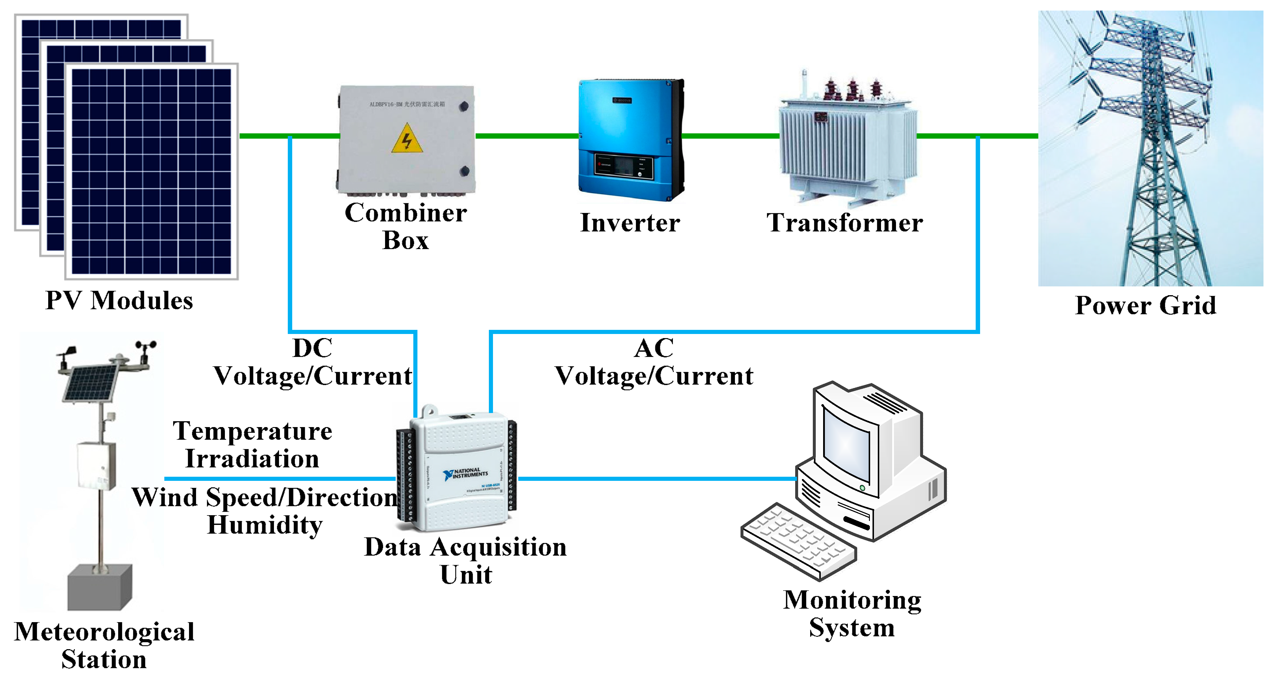
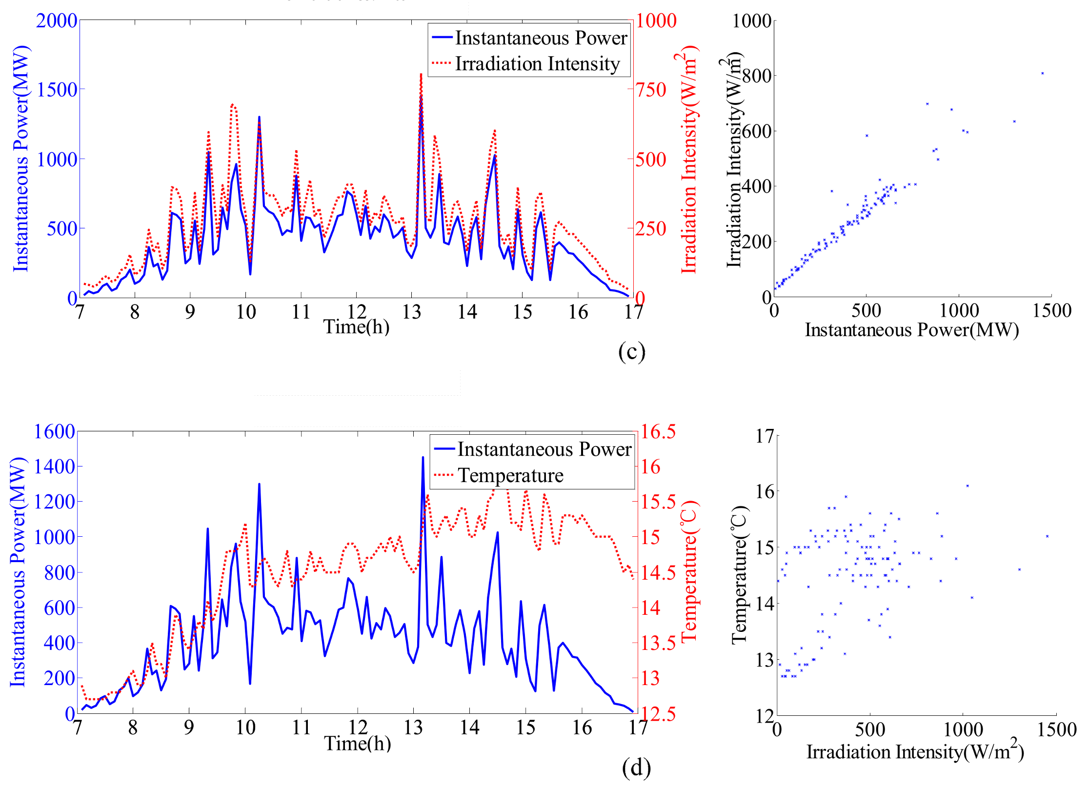
2. Correlation Analysis of PV Generation Factors

Generally, geographical location and meteorological conditions strongly affect the generation of PV power stations. However, the geographical location of a PV power station, layout and arrangement of PV cell panels, global system efficiency and other factors known before the construction of a PV power plant affect generation. Therefore, only the local meteorological conditions are adopted for modeling PV power generation. To reflect the operational status over time, online monitoring systems have been widely applied in many PV power stations. Figure 1 depicts the scheme of a monitoring system that can collect important electrical and meteorological information.
Specifically, these meteorological data include the irradiation intensity, temperature, wind speed and direction, etc. In theory, meteorological factors, especially the irradiation intensity and temperature, have influence on the instantaneous power generation of a PV power station. Figure 2 shows the curve and scatter of the irradiation intensity, temperature and instantaneous power under different sunny and cloudy days. From the scatter diagram, an obvious linear relation between radiation intensity and instantaneous power is shown on both sunny and cloudy days. However, there is not a clear relationship between temperature and instantaneous power. Meanwhile, weather type has a certain influence on this relationship. For example, the scatter points are more concentrated on sunny rather than cloudy days. Therefore, a strong positive correlation exists between the radiation intensity and instantaneous power, while temperature has a weaker correlation with instantaneous power.
The selection of reasonable data is a prerequisite for building an accurate regression model. As shown in Figure 2, the irradiation intensity and temperature directly influences power generation in all weather conditions. In addition, to improve the computational accuracy and efficiency, other monitoring meteorological data must be considered. Therefore, it is necessary to perform correlation analysis to independently explore the correlation degrees between meteorological factors and instantaneous power. Pearson correlation analysis is chosen in this study, and the related results are shown in Table 1. Note that the sine and cosine values of wind direction are adopted.
Table 1 shows that irradiation intensity and temperature have higher correlations with power generation than others do. Moreover, the correlations of wind speed and direction are sufficiently small and can be eliminated from the regression model. As a result, irradiation intensity and temperature are adopted as the training datasets of the SVR model.

3. Hybrid Forecasting Model

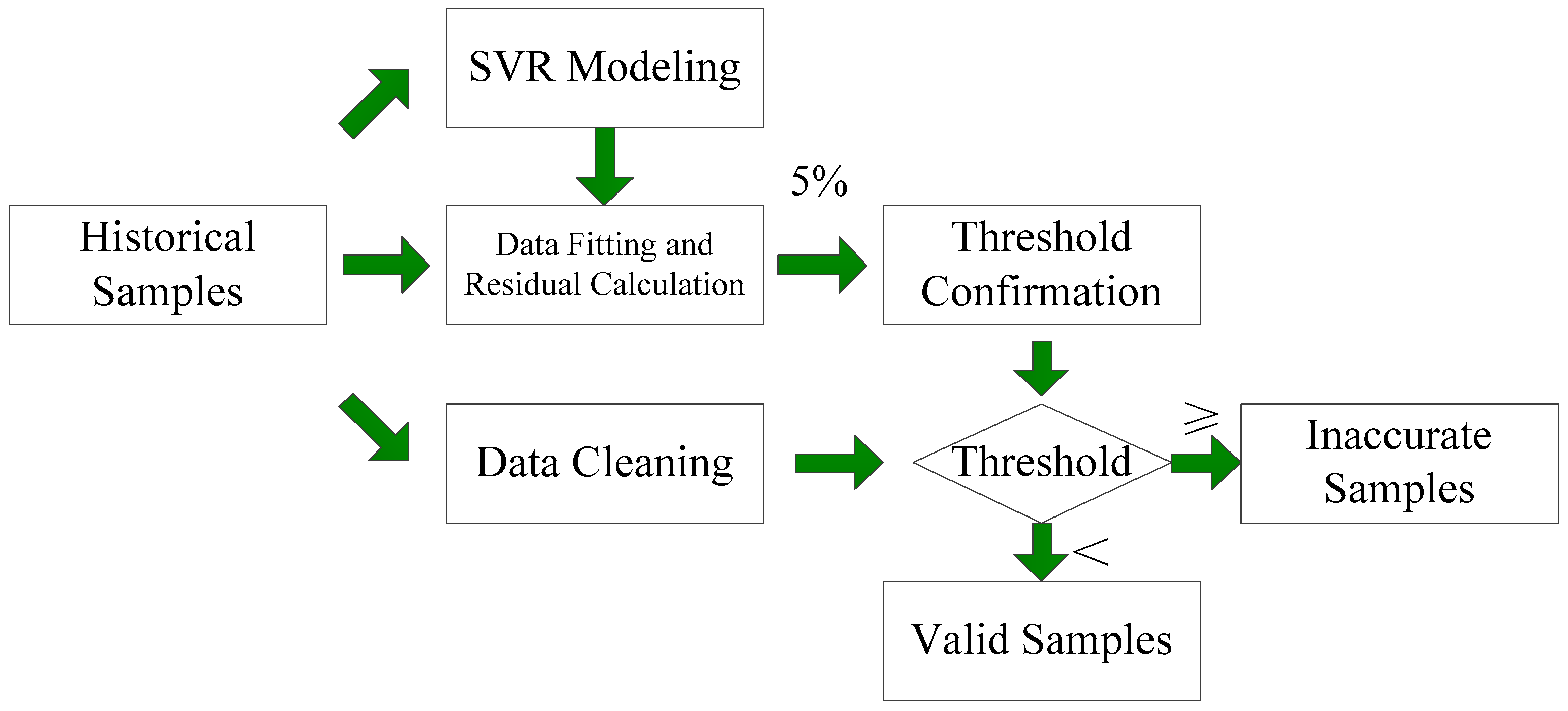
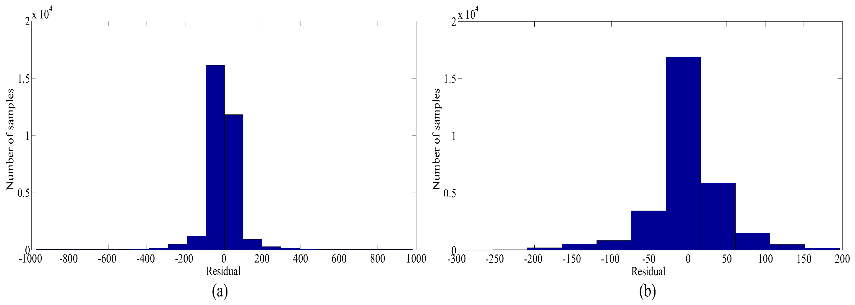
3.1. Data Verification and Cleaning

The training data were collected from a PV power station in Wujiang District, Jiangsu Province, China. This power station has three grid-connected points, and its total installed capacity is 10 MW. Currently, a comprehensive monitoring system has been set up at this station, and nearby independent weather stations collect real-time weather information for the system. Power metering devices are installed at grid-connected points to collect power information, which is sampled at an interval of 5 min. The period of the modeling data spans from April 2016 to February 2017, for almost a total of nine months, amounting to 295 days. There are 31,397 samples when nighttime samples with instantaneous power values of 0 are removed. The samples [ T i , I R i , P i ] include temperature T i , irradiation intensity I R i and instantaneous power P i . Generally, some inaccurate data exist in a database due to sensor failure, data acquisition module failure and system error. These data have negative effects on weather pattern recognition and regression modeling. Therefore, they must be eliminated in advance. In this paper, the inaccurate and incorrect data are cleaned using residual processing based on SVR. As noted in Table 1, P i has a relatively high relationship with I R i and T i . Thus, P i and P j ( P i and P j are ith and jth samples) should not significantly deviate over similar ranges of I R i , I R j and T i , T j . Otherwise, these samples can be regarded as incorrect samples. Figure 3 shows the data cleaning process. First, all the historical samples are used to establish the SVR model with inputs I R i and T i and output P i . Then, fitting residuals can be calculated. Second, the samples with maximum residuals of 5% are considered to be inaccurate and are used to establish a corresponding threshold. Finally, samples are eliminated if their residuals are greater than the threshold. Remaining samples are used in the forecasting model.

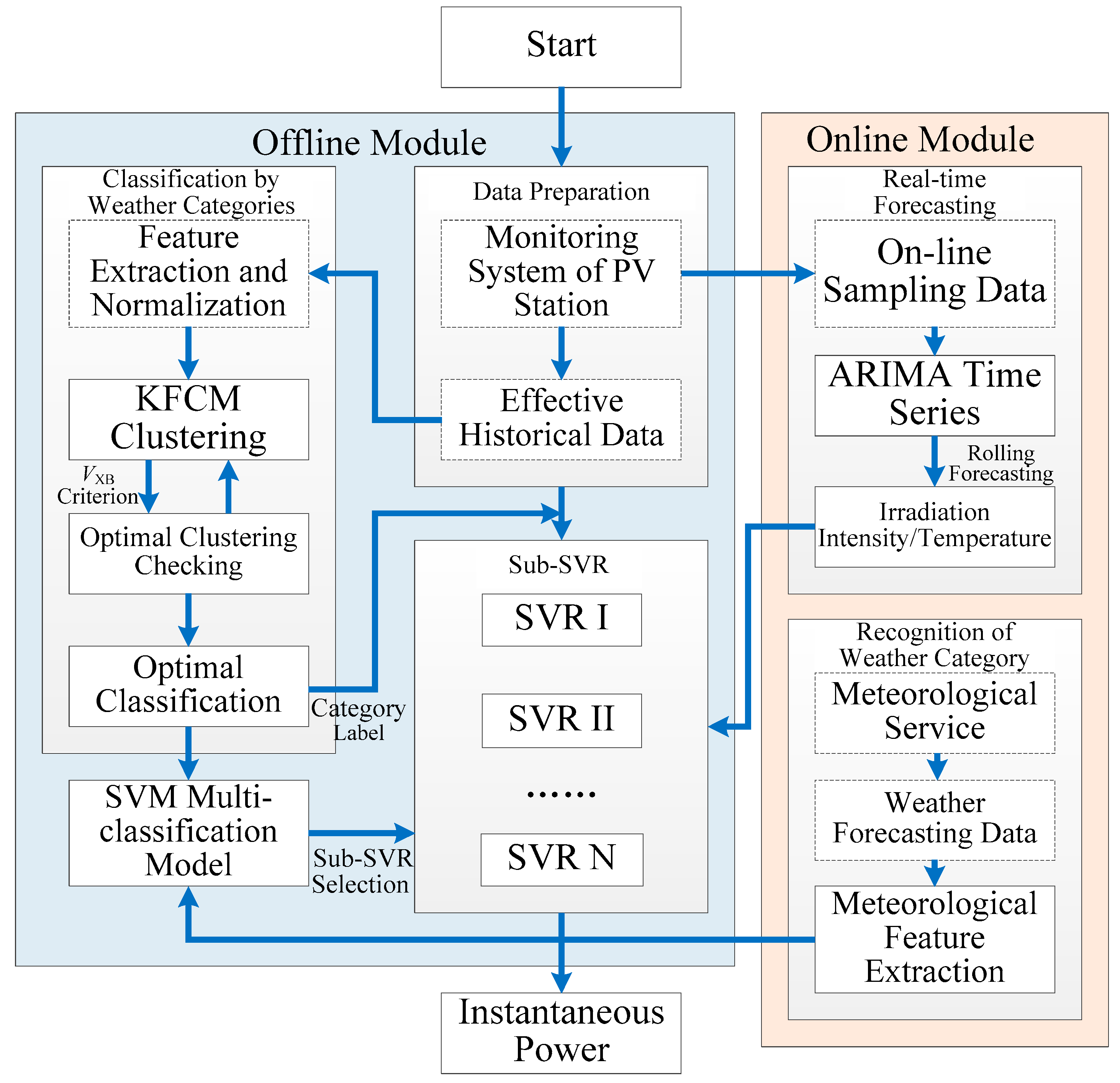
3.2. Hybrid Forecasting Model

The hybrid forecasting model contains an offline module for historical data processing and an online module for real-time forecasting. The integrated model is shown in Figure 4. The main functions of the offline module are as follows:
  • the classification of historical samples according to meteorological characteristics;
  • the establishment of regression submodels (sub-SVRs);
  • the effective identification of weather types and selection of sub-SVRs.
The main functions of the online module are as follows:
  • the forecasting of irradiation intensities and temperatures in rolling mode;
  • the real-time forecasting of instantaneous power generation for a PV station.
Rolling forecasting is a forecasting mode. Predicted value can be obtained by a time series model. Simultaneously, this time series model can be extended and corrected by the actual value for further forecasting step by step.
Data verification and cleaning, weather identification and sub-SVRs establishment are all included in the offline module, while time series forecasting and regression are performed in the online module. The classified regression model has better accuracy than the overall model due to the advantage of eliminating the interference of unknown factors on other weather conditions. In this paper, KFCM and SVM are selected to identify weather types. The real-time forecasting of irradiation intensity and temperature is achieved using the ARIMA method. The instantaneous power of the PV station is obtained using sub-SVRs. The processing steps are as follows:
Step 1.
Meteorological feature selection: The feature vectors [ I R max , T max , D I F F IRmax , M V IR , S T D IR , T D IRmax ] of the KFCM model are calculated. I R max is the maximum irradiance, and T max is the maximum temperature. D I F F IRmax , M V IR , S T D IR and T D IRmax are the maximum fluctuation, mean fluctuation, standard deviation of fluctuate on and maximum third derivative, respectively. They are standardized by the Z-score method.
Step 2.
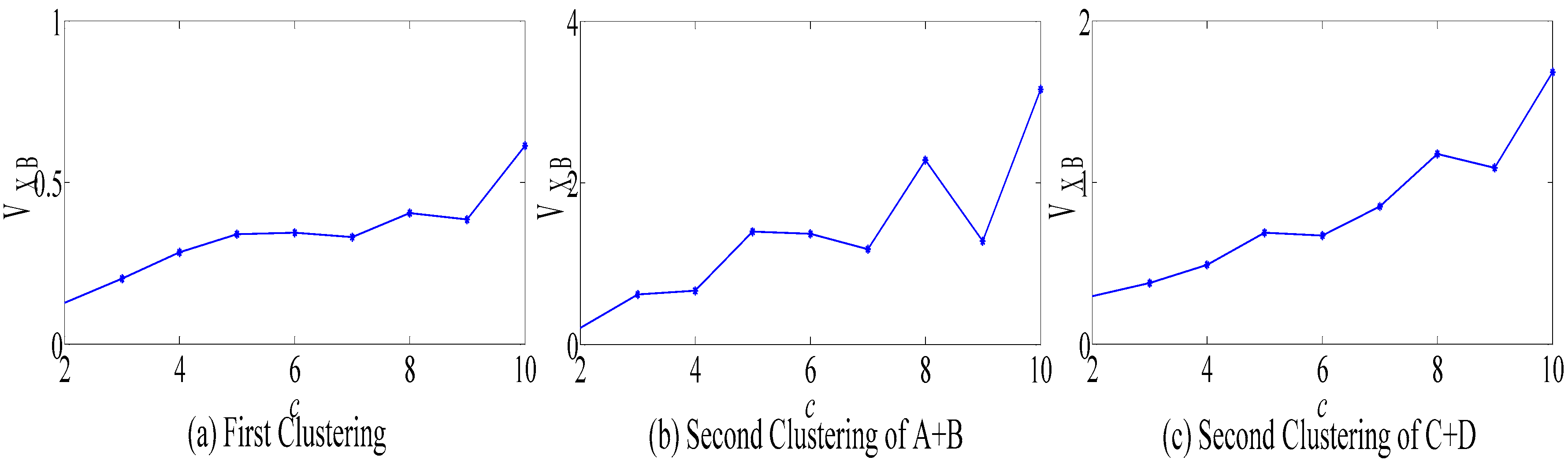
Clustering and optimization: An unsupervised clustering model is established using KFCM. In addition, the VXB indicator is selected to determine the optimal clustering number. Both historical samples and meteorological features are denoted by category labels.
Step 3.
Establishment of the sub-SVR model: the historical samples in one category are used to construct the SVR submodel. Additionally, several submodels are established.
Step 4.
Multiclassification modeling: An SVM recognition model is established using meteorological features. To obtain the category attributes on target days, the features calculated from the NWP service are input into the SVM model. Corresponding submodels are selected according to the category label of the target day.
Step 5.
Time series modeling: The ARIMA time series model is established using some data, including T and I R , collected by the online PV monitoring system on the target day. Then, new predicted values of the time series can be obtained via rolling forecasting.
Step 6.
Instantaneous power forecasting: The predicted values are input into the corresponding sub-SVR models and yield the final instantaneous power P i .

3.3. Feature Selection for Weather Identification

As discussed above, the temperature and irradiation intensity play major roles in PV power generation. Additionally, irradiation fluctuation is the most important factor that influences PV power forecasting due to the random interference caused by meteorological conditions. Therefore, in weather identification, the fluctuation indexes of irradiance are used as the main features in weather clustering under different fluctuation conditions. In this paper, six features are selected for modeling. The first three are as follows:
  • maximum irradiance I R max = max ( I R i ) ,
  • maximum temperature T max = max ( T i ) ,
  • the maximum fluctuation D I F F IRmax = max ( D I F F IR i ) .
Generally, the derivative of irradiance can be used to describe the irradiance fluctuation. However, for discrete data with a constant sampling rate, the first difference D I F F IR is typically adopted to replace the first derivative:
D I F F IR i = I R i + 1 I R i ( i = 1 , 2 , , n 1 ) ,
where n is the number of sampling points. The final three features include the following variables:
  • the fluctuation mean value M V IR , which is the average of D I F F IR i ,
  • the fluctuation standard deviation S T D IR of D I F F IR i , and
  • the maximum third derivative T D IRmax of D I F F IR i . The third derivative is more sensitive to rapid weather changes than are the other derivatives [31].
I R max and T max can reflect maximum instantaneous power. Other features reflect weather fluctuations.
The Z-score method is adopted to eliminate data dimensionality:
x ˜ i = x i x ¯ σ ,
where x i and x ˜ i are the features before and after standardization, respectively, and x ¯ and σ are the mean value and standard deviation of the features.

3.4. KFCM Clustering and Optimization

To classify historical data, feature samples are used to establish the KFCM clustering model. To enhance the separation, the KFCM method transforms the feature space into a high-dimensional space via nonlinear mapping. Therefore, KFCM can overcome the shortcoming of K-means and fuzzy c-means such as local optimum and sensitive to abnormal data. To assess the clustering effectiveness, a cluster validity index must be determined. In this study, the Xie–Beni index [32] V XB is used to evaluate the clustering performance:
V X B = i = 1 C j = 1 n u i j m x j ν i 2 n s s = min j i ν j ν i 2 ,
where C and n are the clustering number and sample number, respectively; u i j is the membership degree; x j is the jth sample; ν i is the ith clustering center; and V XB is the minimum resulting value. At this value, KFCM displays the best performance, and the corresponding value of C is the optimal clustering number. Considering the practical application of model refinement methods, KFCM clustering must be hierarchically executed. Specifically, the first clustering step is executed in accordance with the features ( [ I R max , T max , D I F F IRmax , T D IRmax ] ). Then, the initial results are clustered again with the remaining features ( [ M V IR , S T D IR ] ). The KFCM process is shown in Figure 5.
The process is as follows:
Step 1.
Data preparation: the samples in the first clustering include [ I R max , T max , D I F F IRmax , T D IRmax ] .
Step 2.
The initial clustering number is C = 2.
Step 3.
KFCM is executed as follows:
Step a.
Initialization of KFCM clustering centers ν i ,
Step b.
Membership degrees u i k are calculated by the following equation:
u i k = ( 1 / ( K ( x k , x k ) + K ( ν i , ν i ) 2 K ( x k , ν i ) ) ) 1 / ( m 1 ) j = 1 c ( 1 / ( K ( x k , x k ) + K ( ν j , ν j ) 2 K ( x k , ν j ) ) ) 1 / ( m 1 ) ,
where xk is the sample, and K is the Gaussian kernel function:
K ( x i , x j ) = exp ( x i x j δ 2 ) .
δ is the kernel parameter.
Step c.
New clustering centers are updated as follows:
ν i = k = 1 n u i k m K ( x k , ν i ) x k k = 1 n u i k m K ( x k , ν i ) .
Step d.
KFCM terminal conditions: When the minimum variation in clustering centers ν i or the cycle number threshold is met, the cycle is stopped. Otherwise, the cycle continues from Steps a to d.
Step 4.
The clustering validity coefficient V XB ( C ) is calculated using Formula (3).
Step 5.
C = C + 1; if C C max , proceed to step 3. Otherwise, proceed to step 6.
Step 6.
The optimum clustering number Copt is determined by the minimum VXB(C).
Step 7.
A second clustering process will be executed to classify the results of the first clustering using [ M V IR , S T D IR ] and based on steps 1–6.

3.5. SVM Recognition and the Sub-SVR Model

As a machine learning algorithm, SVM is widely used in data classification, pattern recognition and fault diagnosis. The core concept of SVM is to construct an optimal separating hyperplane so that the distance between the hyperplane and the sample nearest the hyperplane is the maximum distance. For classification problem ( x i , y i ) , i = 1 , 2 , , l , x i R n , y i { 1 , + 1 } , samples can be accurately separated into two categories by the optimal hyperplane w · x + b = 0 . Therefore, the construction of the optimal hyperplane can be transformed into an optimization problem:
min w , b 1 2 w 2 + c i = 1 l ξ i .
The SVM constraint condition is given by Label (8):
y i ( ( w · x i ) + b ) 1 ξ i , i = 1 , 2 , , l ,
where w is the normal vector of the optimal hyperplane and b , c , and ξ i , are the threshold, penalty parameter and slack variable, respectively.
The Lagrange multiplier method can be used to solve this optimization problem. For nonlinear classification, samples in low-dimensional space are mapped into high-dimensional space using the function ϕ ( x ) . The kernel function K ( x i , x j ) is the same as that used in the KFCM method. The objective function can be expressed as follows:
max . L = i = 1 l α i 1 2 i , j = 1 l α i α j y i y j K ( x i , x j ) ,
where α i is the Lagrange multiplier.
SVR is an important branch of SVM. The main concept of SVR is to map linearly inseparable samples into high-dimensional space for linear regression. Ultimately, the nonlinear regression function f ( x ) = w T φ ( x ) + b can be obtained. The sub-SVR model in this paper is a combination of several independent SVR models.

3.6. ARIMA Model

Generally, the ARIMA model can be expressed as ARIMA(p, q, d), where p is the autoregressive order, q is the moving average order, and d is the difference order. The ARIMA process is as follows:
Step 1.
Differential processing: The stationary time series data [XAt] are obtained from the original time series [Xt] based on a difference method. In this paper, two ARIMAs are established based on the irradiance intensity sequence [Xt-IR] and the temperature sequence [Xt-T].
Step 2.
Model identification and p and q confirmation: An autocorrelation function (ACF) and a partial correlation function (PACF) are calculated for [XAt]. Then, the model type (AR, MA, or ARMA) will be determined according to the ACF and PACF. In general, the ARIMA model can be expressed as follows:
X A t = i = 1 p a i X A t i + j = 0 q b j e t j ,
where a i is the autoregressive coefficient, b j is the moving average coefficient, and e t j is a white noise series, which represents independent error. The Akaike information criterion (AIC) is commonly used to confirm p and q.
Step 3.
Parameter estimation: After parameter estimation, ARIMA(p, q, d) is established.
Step 4.
Data forecasting: Single-step forecasting is performed to obtain predictions of the irradiance intensity and temperature using the ARIMA model.
Rolling forecasting is adopted for the ARIMA method in this paper because it uses monitoring data to correct the real-time ARIMA model and improve the forecasting accuracy. In this paper, the sampling interval of the PV monitoring system is 5 min. Therefore, the predictive value is acquired by ARIMA model at a 5-min interval. For example, the temperature sequence T i ( i = 1 , 2 , , n ) is the first n monitoring samples on the target day. First, the ARIMA forecasting model is established using T i . Then, the predicted temperature value T n + 1 can be obtained. Second, actual monitoring sample T n + 1 can be acquired 5 min later and is added to T i ( i = 1 , 2 , , n ) to update the ARIMA model. Finally, the next predicted value T n + 2 is obtained by the new ARIMA model, and the model is updated again. The remainder of the process is performed in the same manner.

4. Modeling and Evaluation

According to the data cleaning and modeling processes described in Section 3.1 and Section 3.2, the PV generation forecasting model is established. Four typical weather conditions, sunny (21 July), cloudy (19 May), rainy (7 June) and overcast (22 August), are selected as the test dataset (586 samples). The remaining 30,811 samples are used as the training dataset.

4.1. Data Verification and Cleaning Based on SVR

As shown in Figure 3, the sub-SVR model should be established using the training dataset with irradiation intensity I R i and temperature T i inputs and instantaneous power P i as the output. The model parameters should be optimized using a cross-validation method. Penalty parameter c and kernel parameter g are set to 194.02 and 0.0098, respectively. Then, the training samples are fitted by the SVR model to calculate the residuals. Finally, the residuals are ranked in descending order. The samples in the highest 5% of residuals are removed as abnormal samples, and the remaining samples are regarded as valid samples. To evaluate the fitting precision of PV instantaneous power, the mean absolute percentage error ( ε MAPE ) is chosen to measure the global error, while the root mean square error ( ε RMSE ) is chosen to measure the difference between predicted and real values. The histograms of the residual distribution before and after cleaning are shown in Figure 6. ε MAPE and ε RMSE are shown in Table 2:
ε MAPE = 100 n i = 1 n | P i P i P i | % ,
ε RMSE = 1 n i = 1 n ( P i P i ) 2 .
Figure 6 and Table 2 show that ε MAPE and ε RMSE decrease, and the residual distribution becomes more reasonable.

4.2. Weather Identification and Regression Submodel Establishment

After data cleaning, daily meteorological features are extracted from the modeling dataset using the methods presented in Section 3.3. Notably, 261 valid days are used ( [ I R max , T max , D I F F IRmax , M V IR , S T D IR , T D IRmax ] ). These feature days are categorized to label the modeling data. Next, a hierarchical clustering model is established, as discussed in Section 3.4. In general, an overly large clustering number can negatively affect the clustering performance. Therefore, the maximum clustering number is set to Cmax = 10. The variation of V XB is shown in Figure 7. Notably, when C = 2, V XB is at a minimum. Therefore, the optimal clustering number of the two layers is 2. Moreover, all the feature days are divided into four categories. The clustering results are shown in Table 3.
After labeling the 261 feature days, these days are used to establish the multiclassification SVM model for weather type identification. Specifically, 183 days are selected for training, and the remaining 78 days are used as the test dataset. Through cross-validation, the penalty parameter c = 111.4305 and the kernel parameter g = 0.00156 are obtained. The results of the weather type test are shown in Table 4.
In Table 4, the SVM model misclassifies four days that belong to category B, resulting in a 94.78% classification accuracy. Thus, the SVM accuracy is high enough for weather recognition, and this model can identify the weather types on target days. Therefore, corresponding sub-SVR models can be reasonably selected.

4.3. ARIMA Time Series Forecasting and Sub-SVRs

According to Section 3.2, two essential steps should be completed by the online module: sub-SVR selection and regression and ARIMA modeling and forecasting.
In the first step, 29,829 data samples over 261 days are classified into A, B, C and D classes by KFCM. The sub-SVR model is established using samples with the same label. Four submodels (SUB-A, SUB-B, SUB-C and SUB-D) with irradiation intensity I R i and temperature T i inputs and output instantaneous power P i as the output are obtained. Subsequently, weather type identification is performed. The weather information on target days is input into the SVM multiclassification model to obtain the category attribute. The target days selected include 19 May, 7 June, 21 July, and 22 August. The category labels obtained for these four days using the SVM model are B, C, D and B, which correspond to submodels SUB-B, SUB-C, SUB-D and SUB-B, respectively.
In the second step, the hybrid forecasting models based on ARIMA time series and sub-SVR are established in accordance with the process described in Section 3.6, and rolling forecasting is adopted. To meet the requirements of time series modeling and engineering applications, two ARIMA models are established using the first 20 values of I R i and T i (I = 1~20), which are obtained from the online PV monitoring system on the target days. The sampling interval is 5 min. For example, on 21 July, the first monitoring values appeared at 6:15 a.m. The first 20 monitoring values ( I R i , T i ) are collected from 6:15 a.m. to 7:55 a.m. Then, ARIMA modeling and forecasting begin. Subsequently, two time series models, ARIMAIR and ARIMAT, can be constructed to forecast irradiation intensity and temperature, respectively. Model parameters p, q and d are set to 1. Then, the subsequent values of I R i + 1 and T i + 1 (5 min later at 8:00 a.m.) can be predicted using the ARIMAIR and ARIMAT models. These predicted values are input into the submodel SUB-D to obtain the predicted instantaneous power P i + 1 . In addition, the new actual monitoring values I R i + 1 and T i + 1 can be used in real time to modify the ARIMAIR and ARIMAT models. I R i + 1 and T i + 1 are obtained from the PV monitoring system at 8:00 a.m. Then, the next predicted values, I R i + 2 , T i + 2 and P i + 2 (8:05 a.m.), can be similarly obtained. The instantaneous power P is forecasted in real time via a rolling cycle. The forecasts of I R and T and the regression of P by the hybrid forecasting models on four target days are shown in Figure 8, Figure 9 and Figure 10. Additionally, the forecasting accuracy is shown in Table 5. Moreover, for comparison of different forecasting algorithms, four different regression models are established: the sub-SVR model, a global SVR model (G-SVR), a back propagation neural network submodel (S-BPNN) and a global BPNN model (G-BPNN). The global models are established using all the training data, while submodels are established using the classified data. The forecasting results are shown in Table 6.
The following conclusions can be obtained from the forecasting results:
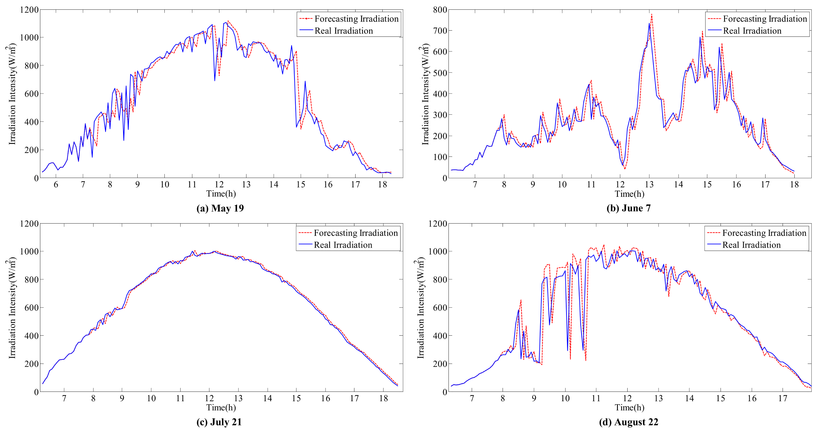
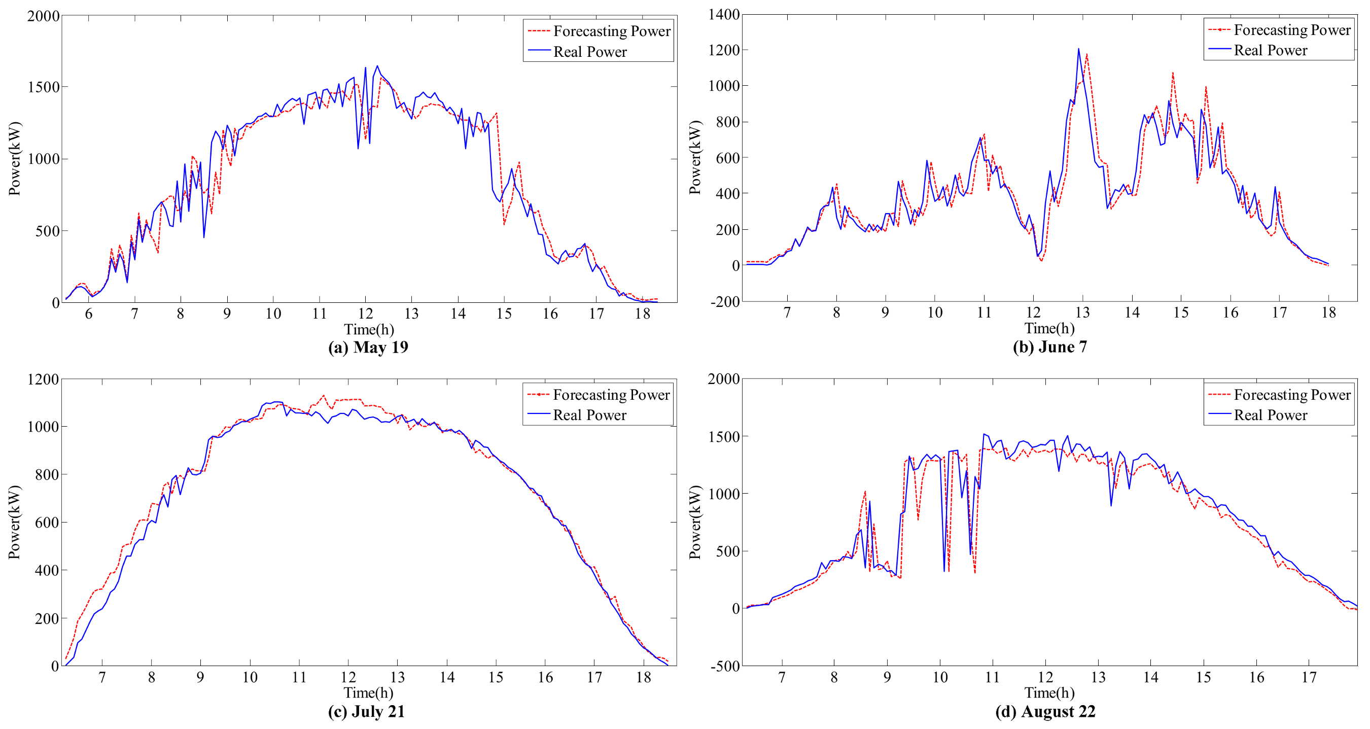
  • The accurate forecasting results of IR and T can be used as inputs in the sub-SVR to improve the forecasting performance of P. As a result, the forecasted and actual curves are similar.
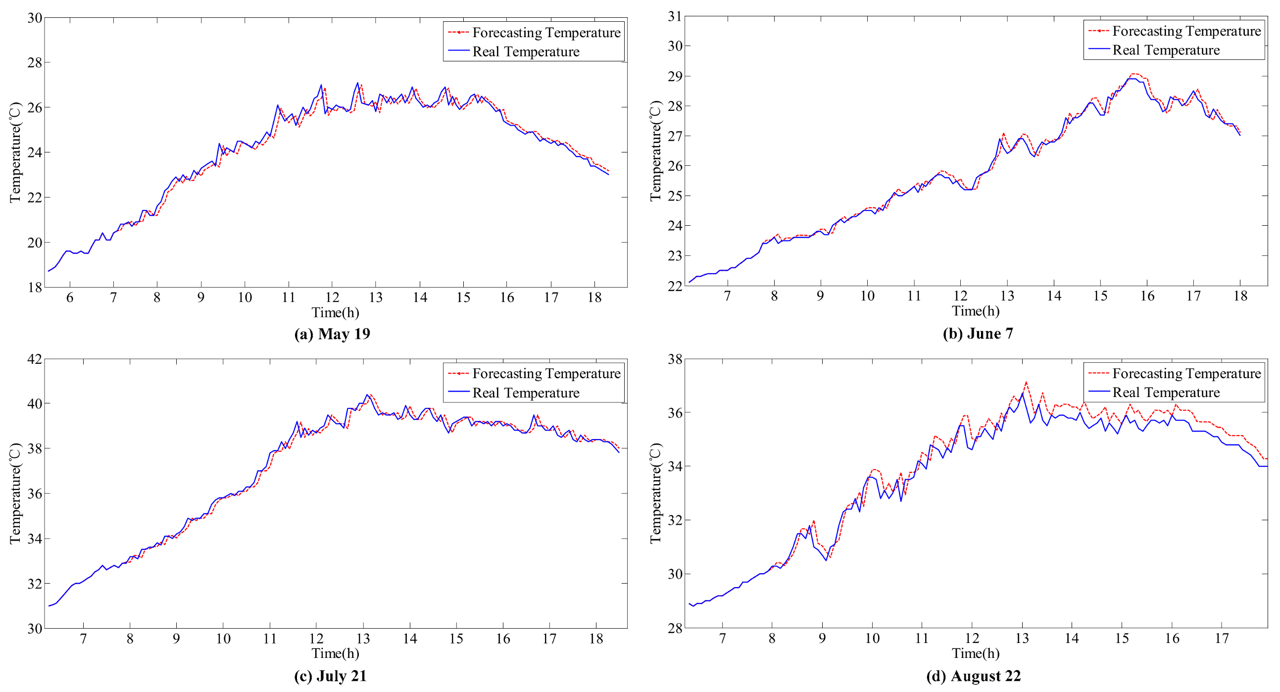
  • IR and T are relatively stable on the sunny day (21 July), and the variation trends are clear. Reasonable forecasting results can be obtained with the ARIMA models. The curves of forecasted IR and T are coincident with the actual monitoring curves on the sunny day. However, in other weather conditions, errors can be observed in the forecasting results for various reasons.
  • The effect of variations in T on P is considered in this hybrid model. For instance, on 21 July, the peak value of IR occurs at approximately 12 p.m. However, the peak value of P appears between 10 p.m. and 11 p.m. On one hand, IR is stable and does not considerably affect the fluctuation in P. On the other hand, the increase in temperature during this period decreases P. This result is reflected by the forecasting curve in Figure 8, Figure 9 and Figure 10c.
  • In the ARIMA models, T is more stable than IR under all weather conditions, with higher forecasting accuracy. However, the correlation between IR and P is higher than the correlation between T and P. Thus, the influence of IR on P is larger than that of T. Meanwhile, volatility will considerably affect the time series fitting ability of ARIMA. Therefore, the forecasting accuracy of the hybrid model depends on the processing of IR volatility.
Generally, SVR has an advantage in processing fluctuant data relative to BPNN. However, because it is sunny on 21 July, T and IR are more stable than other days, and forecasting performances of G-BPNN and G-SVR are approximate. Except for this day, the G-SVR model has better fitting and forecasting ability than the G-BPNN model. Moreover, the submodels can improve the forecasting accuracy by excluding interference factors under different weather conditions. Therefore, the hybrid forecasting model proposed is a reasonable choice.

5. Conclusions

Grid dispatching and power quality are impacted where the large number of PV systems are connected to power grid. Control and regulation of the power balance between PV power generation and other energy power generation are the main problem of power grids. In this paper, the ultrashort-term forecasting model of PV power station generation can provide reliable information for the grid dispatching system every 5 min in time. It is an effective method of improving the coordinated control and enhancing the consumption capacity of PV energy. In this paper, irradiation intensity and temperature are selected to establish the hybrid forecasting model for weather type identification and time series analysis. KFCM and SVM are used in the classification and identification of weather types, respectively. SVR submodels and an ARIMA model are constructed for the real-time tracking and reconstruction of the forecasting model, respectively. The data analysis yielded the following results:
  • The hybrid forecasting model is established based on actual monitoring data from a PV power station. These data reflect the actual meteorological and working conditions of the PV station in real time. Rolling forecasting is adopted to correct the ARIMA model using real-time data. Meanwhile, the hybrid model exhibits good agreement with the online monitoring system and displays high accuracy.
  • The data fitting accuracy was improved by excluding abnormal data through data preprocessing, including data cleaning and correction processes. Correlation analysis was used to determine the inputs of the forecasting model and improve the calculation efficiency by simplifying the model.
Based on the test results, errors in the hybrid forecasting model increased as irradiation fluctuations increased. Therefore, improving observations of these fluctuations will be emphasized in future research.

Acknowledgments

This work was supported by the China Postdoctoral Science Foundation under Grant No. 2015M571654 and the “111” project of “Renewable Energy and Smart Grid” (B14022).

Author Contributions

Yi Pan and Kedong Zhu conceived and designed the experiments; Yi Pan performed the experiments; Fei Mei analyzed the data; Jianyong Zheng contributed reagents/materials/analysis tools; and Fei Mei wrote the paper.

Conflicts of Interest

The authors declare no conflict of interest.

References

  1. Liu, J.P.; Long, Y.; Song, X.H. A Study on the Conduction Mechanism and Evaluation of the Comprehensive Efficiency of Photovoltaic Power Generation in China. Energies 2017, 10, 723. [Google Scholar] [CrossRef]
  2. National Energy Administration. Photovoltaic Power Generation Statistics in 2015. Available online: http://www.nea.gov.cn/2016-02/05/c_135076636.htm (accessed on 2 June 2016).
  3. Juamperez, M.; Yang, G.Y.; Kjaer, S.B. Voltage regulation in LV grids by coordinated volt-var control strategies. J. Mod. Power Syst. Clean Energy 2014, 2, 319–328. [Google Scholar] [CrossRef] [Green Version]
  4. Yang, G.Y.; Marra, F.; Juamperez, M.; Kjaer, S.B.; Hashemi, S.; Ostergaard, J.; Ipsen, H.H.; Frederiksen, K.H.B. Voltage rise mitigation for solar PV integration at LV grids: Studies from PVNET. dk. J. Mod. Power Syst. Clean Energy 2015, 3, 411–421. [Google Scholar] [CrossRef] [Green Version]
  5. Pinto, R.; Mariano, S.; Calado, M.; Souza, J.D. Impact of Rural Grid-Connected Photovoltaic Generation Systems on Power Quality. Energies 2017, 9, 723. [Google Scholar] [CrossRef]
  6. Gao, Y.; Zhang, B.L.; Mao, J.L.; Liu, Y. Machine Learning-Based Adaptive Very-Short-Term Forecast Model for Photovoltaic Power. Power Syst. Technol. 2015, 39, 307–311. [Google Scholar] [CrossRef]
  7. De Giorgi, M.G.; Congedo, P.M.; Malvoni, M. Photovoltaic power forecasting using statistical methods: Impact of weather data. IET Sci. Meas. Technol. 2014, 8, 90–97. [Google Scholar] [CrossRef]
  8. Mellit, A.; Pavan, A.M.; Lughi, V. Short-term forecasting of power production in a large-scale photovoltaic plant. Sol. Energy 2014, 105, 401–413. [Google Scholar] [CrossRef]
  9. Ehsan, R.M.; Simon, S.P.; Venkateswaran, P.R. Day-ahead forecasting of solar photovoltaic output power using multilayer perceptron. Neural Comput. Appl. 2017, 28, 3981–3992. [Google Scholar] [CrossRef]
  10. Shi, J.; Lee, W.J.; Liu, Y.Q.; Yang, Y.P.; Wang, P. Forecasting Power Output of Photovoltaic Systems Based on Weather Classification and Support Vector Machines. IEEE Trans. Ind. Appl. 2012, 48, 1064–1069. [Google Scholar] [CrossRef]
  11. De Giorgi, M.G.; Congedo, P.M.; Malvoni, M.; Laforgia, D. Error analysis of hybrid photovoltaic power forecasting models: A case study of mediterranean climate. Energy Convers. Manag. 2015, 100, 117–130. [Google Scholar] [CrossRef]
  12. Li, Y.T.; He, Y.; Su, Y.; Shu, L.J. Forecasting the daily power output of a grid-connected photovoltaic system based on multivariate adaptive regression splines. Appl. Energy 2016, 180, 392–401. [Google Scholar] [CrossRef]
  13. Marquez, R.; Coimbra, C.F.M. Intra-hour DNI forecasting based on cloud tracking image analysis. Sol. Energy 2013, 91, 327–336. [Google Scholar] [CrossRef]
  14. Yang, H.D.; Kurtz, B.; Nguyen, D.; Urquhart, B.; Chow, C.W.; Ghonima, M.; Kleissl, J. Solar irradiance forecasting using a ground-based sky imager developed at UC San Diego. Sol. Energy 2014, 103, 502–524. [Google Scholar] [CrossRef]
  15. Escrig, H.; Batlles, F.J.; Alonso, J.; Baena, F.M.; Bosch, J.L.; Salbidegoitia, I.B.; Burgaleta, J.I. Cloud detection, classification and motion estimation using geostationary satellite imagery for cloud cover forecast. Energy 2013, 55, 853–859. [Google Scholar] [CrossRef]
  16. Voyant, C.; Muselli, M.; Paoli, C.; Nivet, M.L. Numerical weather prediction (NWP) and hybrid ARMA/ANN model to predict global radiation. Energy 2012, 39, 341–355. [Google Scholar] [CrossRef]
  17. Bouzerdoum, M.; Mellit, A.; Pavan, A.M. A hybrid model (SARIMA-SVM) for short-term power forecasting of a small-scale grid-connected photovoltaic plant. Sol. Energy 2013, 98, 226–235. [Google Scholar] [CrossRef]
  18. Chen, S.X.; Gooi, H.B.; Wang, M.Q. Solar radiation forecast based on fuzzy logic and neural networks. Renew. Energy 2013, 60, 195–201. [Google Scholar] [CrossRef]
  19. Li, J.M.; Ward, J.K.; Tong, J.N.; Collins, L.; Platt, G. Machine learning for solar irradiance forecasting of photovoltaic system. Renew. Energy 2016, 90, 542–553. [Google Scholar] [CrossRef]
  20. Yang, D.Z.; Kleissl, J.; Gueymard, C.A.; Pedro, H.T.C.; Coimbra, C.F.M. History and trends in solar irradiance and PV power forecasting: A preliminary assessment and review using text mining. Sol. Energy 2018. [Google Scholar] [CrossRef]
  21. Antonanzas, J.; Osorio, N.; Escobar, R.; Urraca, R.; Martinez-de-Pison, F.J.; Antonanzas-Torres, F. Review of photovoltaic power forecasting. Sol. Energy 2016, 136, 78–111. [Google Scholar] [CrossRef]
  22. Raza, M.Q.; Nadarajah, M.; Ekanayake, C. On recent advances in PV output power forecast. Sol. Energy 2016, 136, 125–144. [Google Scholar] [CrossRef]
  23. Inman, R.H.; Pedro, H.T.C.; Coimbra, C.F.M. Solar forecasting methods for renewable energy integration. Prog. Energy Combust. Sci. 2013, 39, 535–576. [Google Scholar] [CrossRef]
  24. Eseye, A.T.; Zhang, J.H.; Zheng, D.H. Short-term photovoltaic solar power forecasting using a hybrid Wavelet-PSO-SVM model based on SCADA and Meteorological information. Renew. Energy 2018, 118, 357–367. [Google Scholar] [CrossRef]
  25. Bae, K.Y.; Jang, H.S.; Sung, D.K. Hourly Solar Irradiance Prediction Based on Support Vector Machine and Its Error Analysis. IEEE Trans. Power Syst. 2017, 32, 935–945. [Google Scholar] [CrossRef]
  26. Lai, C.S.; Jia, Y.W.; McCulloch, M.D.; Xu, Z. Daily Clearness Index Profiles Cluster Analysis for Photovoltaic System. IEEE Trans. Ind. Inform. 2017, 13, 2322–2332. [Google Scholar] [CrossRef]
  27. Yang, H.T.; Huang, C.M.; Huang, Y.C.; Pai, Y.S. A Weather-Based Hybrid Method for 1-Day Ahead Hourly Forecasting of PV Power Output. IEEE Trans. Sustain. Energy 2014, 5, 917–926. [Google Scholar] [CrossRef]
  28. Wang, J.D.; Ran, R.; Song, Z.L.; Sun, J.W. Short-Term Photovoltaic Power Generation Forecasting Based on Environmental Factors and GA-SVM. J. Electr. Eng. Technol. 2017, 12, 64–71. [Google Scholar] [CrossRef]
  29. Wang, F.; Zhen, Z.; Mi, Z.Q.; Sun, H.B.; Su, S.; Yang, G. Solar irradiance feature extraction and support vector machines based weather status pattern recognition model for short-term photovoltaic power forecasting. Energy Build. 2015, 86, 427–438. [Google Scholar] [CrossRef]
  30. Dong, Z.B.; Yang, D.Z.; Reindl, T.; Walsh, W.M. A novel hybrid approach based on self-organizing maps, support vector regression and particle swarm optimization to forecast solar irradiance. Energy 2015, 82, 570–577. [Google Scholar] [CrossRef]
  31. Wang, F.; Mi, Z.Q.; Zhen, Z.; Yang, G.; Zhou, H.M. A Classified Forecasting Approach of Power Generation for Photovoltaic Plants Based on Weather Condition Pattern Recognition. Proc. CSEE 2013, 33, 75–82. [Google Scholar] [CrossRef]
  32. Li, H.P.; Zhang, S.Q.; Ding, X.H.; Zhang, C.; Dale, P. Performance evaluation of cluster validity indices (CVIs) on multi/hyperspectral remote sensing datasets. Remote Sens. 2016, 8, 295. [Google Scholar] [CrossRef] [Green Version]
Figure 1. Typical structure of an online monitoring system in a PV power station.
Sustainability 10 00820 g001
Figure 2. Comparison of instantaneous power, irradiation intensity and temperature. (a) curve and scatter diagram of instantaneous power and irradiation intensity on sunny days; (b) curve and scatter diagram of instantaneous power and temperature on sunny days; (c) curve and scatter diagram of instantaneous power and irradiation intensity on cloudy days; (d) curve and scatter diagram of instantaneous power and temperature on cloudy days.
Sustainability 10 00820 g002aSustainability 10 00820 g002b
Figure 3. Data cleaning process based on SVR.
Sustainability 10 00820 g003
Figure 4. Hybrid forecasting model of photovoltaic power generation.
Sustainability 10 00820 g004
Figure 5. KFCM modeling process and optimization.
Sustainability 10 00820 g005
Figure 6. Fitting the residual distribution before and after cleaning. (a) the histogram of the residual distribution before cleaning; (b) the histogram of the residual distribution after cleaning.
Sustainability 10 00820 g006
Figure 7. V XB curves of first and second clustering. (a) V XB curves of first clustering; (b) V XB curves of second clustering of A + B; (c) V XB curves of second clustering of C + D.
Sustainability 10 00820 g007
Figure 8. Forecasting results of irradiation intensity for four weather types. (a) forecasting results of irradiation intensity on 19 May; (b) forecasting results of irradiation intensity on 7 June; (c) forecasting results of irradiation intensity on 21 July; (d) forecasting results of irradiation intensity on 22 August.
Sustainability 10 00820 g008
Figure 9. Forecasting results of temperature for four weather types. (a) forecasting results of temperature on 19 May; (b) forecasting results of temperature on 7 June; (c) forecasting results of temperature on 21 July; (d) forecasting results of temperature on 22 August.
Sustainability 10 00820 g009
Figure 10. Forecasting results of power for four weather types. (a) forecasting results of power on 19 May; (b) forecasting results of power on 7 June; (c) forecasting results of power on 21 July; (d) forecasting results of power on 22 August.
Sustainability 10 00820 g010
Table 1. Correlation degrees between meteorological factors and PV power generation.
Meteorological FactorCorrelation
Irradiation intensity0.885
Temperature0.316
Wind speed0.025
Direction (sin)−0.028
Direction (cos)−0.128
Table 2. ε MAPE and ε RMSE before and after cleaning.
Before CleaningAfter Cleaning
ε MAPE 19.38%18.56%
ε RMSE 83.7345.63
Table 3. Clustering results of weather features.
Days Number in Clusters
First clustering118 (A + B)143 (C + D)
Second clustering45 (A)79 (B)39 (C)104 (D)
Table 4. Results of the weather type test based on the SVM model.
Actual CategoryTest CategoryTotal
ABCD
A1000010
B3221026
C0011011
D0003131
Total1322123178
Table 5. Forecasting accuracy of IR and T.
ModelDataObject ε MAPE ε RMSE
ARIMA19 MayIR17.24%105.20
T1.11%0.3373
7 JuneIR18.93%73.70
T0.56%0.1967
21 JulyIR2.35%17.13
T0.52%0.2629
22 AugustIR16.02%152.54
T1.14%0.4634
Table 6. Forecasting accuracy of P.
ModelAccuracy
19 May7 June
ε MAPE ε RMSE ε MAPE ε RMSE
Sub-SVR17.12%142.7120.76%112.77
G-SVR18.33%143.5122.21%112.29
S-BPNN17.48%146.3824.48%117.90
G-BPNN19.09%144.5929.13%114.54
Model21 July22 August
ε MAPE ε RMSE ε MAPE ε RMSE
Sub-SVR4.47%43.3417.00%201.09
G-SVR7.58%56.7117.53%207.78
S-BPNN4.51%42.4020.52%222.25
G-BPNN7.45%55.6224.58%218.42

