Cooperation Modes of Operations and Financing in a Low-Carbon Supply Chain


Abstract
1. Introduction
2. Literature Review
2.1. Carbon Finance and Supply Chain Finance
2.2. Supply Chain Cooperation and Optimization
2.3. Cap-and-Trade Scheme
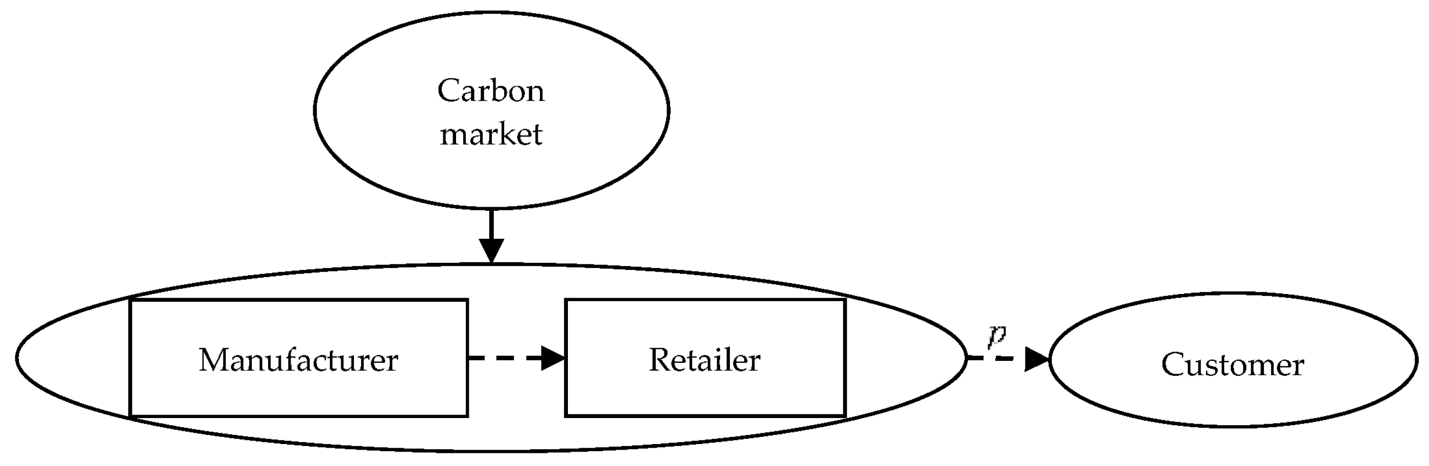
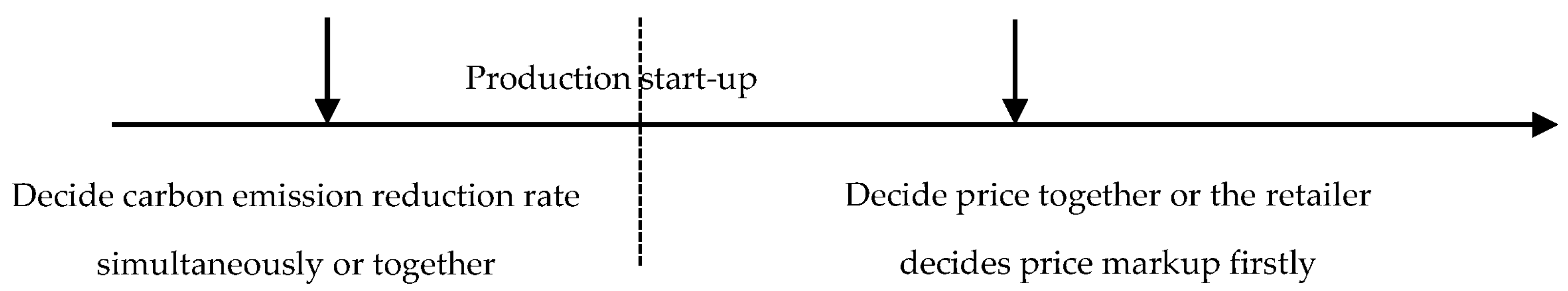
3. Models
3.1. Basic Notations and Preliminaries
3.2. Non-Cooperation with Finance Pattern (NCF)
3.3. Supply Chain Carbon Finance Pattern (SCCF)
3.4. Partial-Cooperation with Delay-in-Payment Pattern (PCD)
3.5. Full Cooperation Pattern (FC)
3.6. Results and Discussion
4. Extensions
4.1. Models
4.2. Results and Discussion
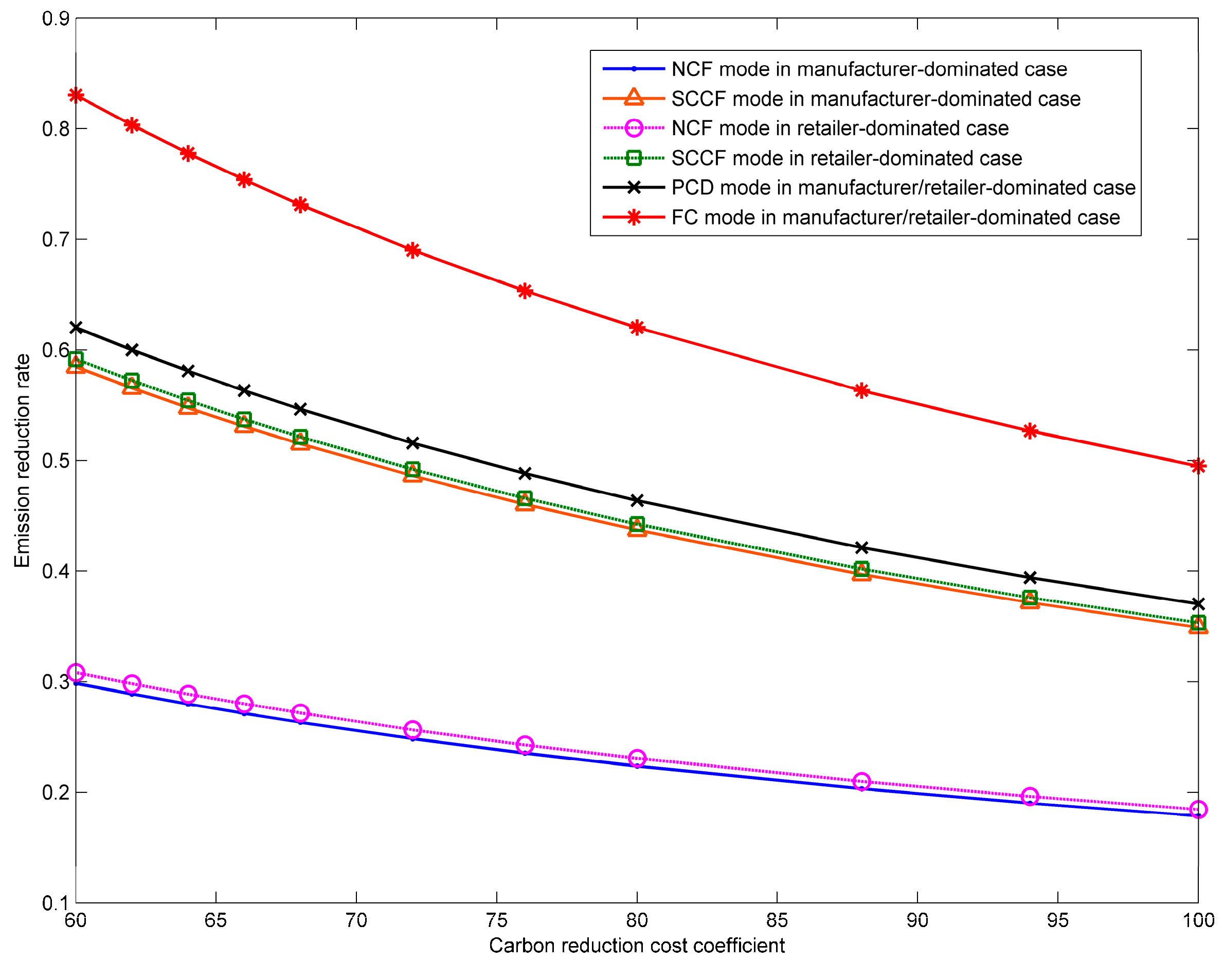
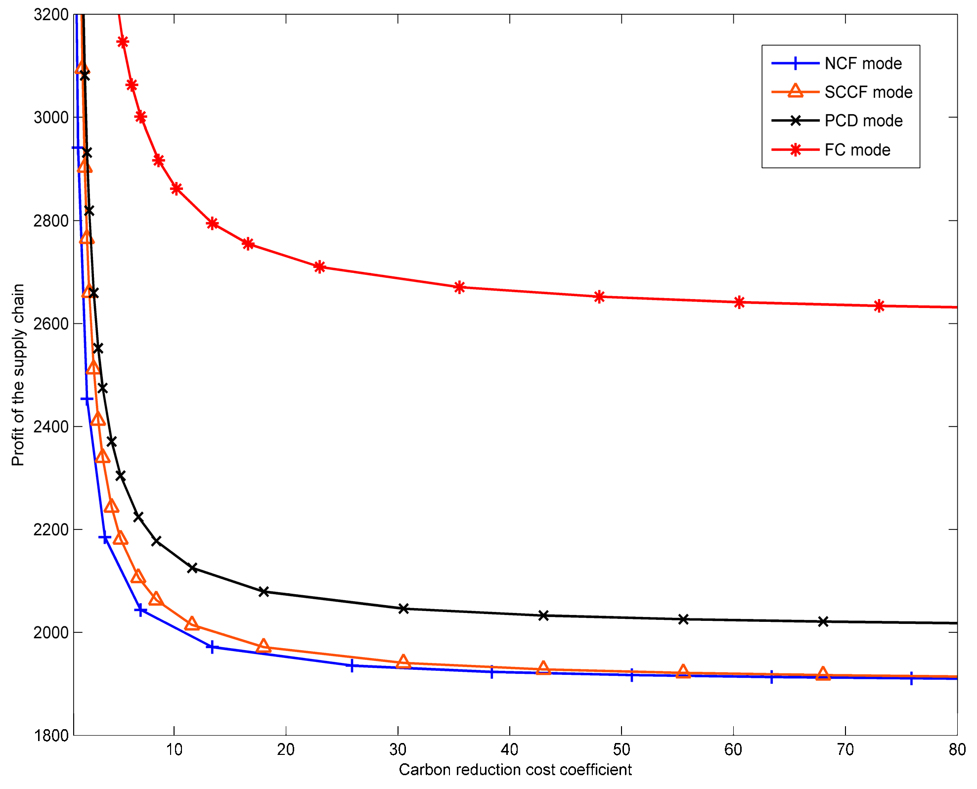
5. Numerical Analysis
5.1. Impact of on Optimal Emission Reduction Rate
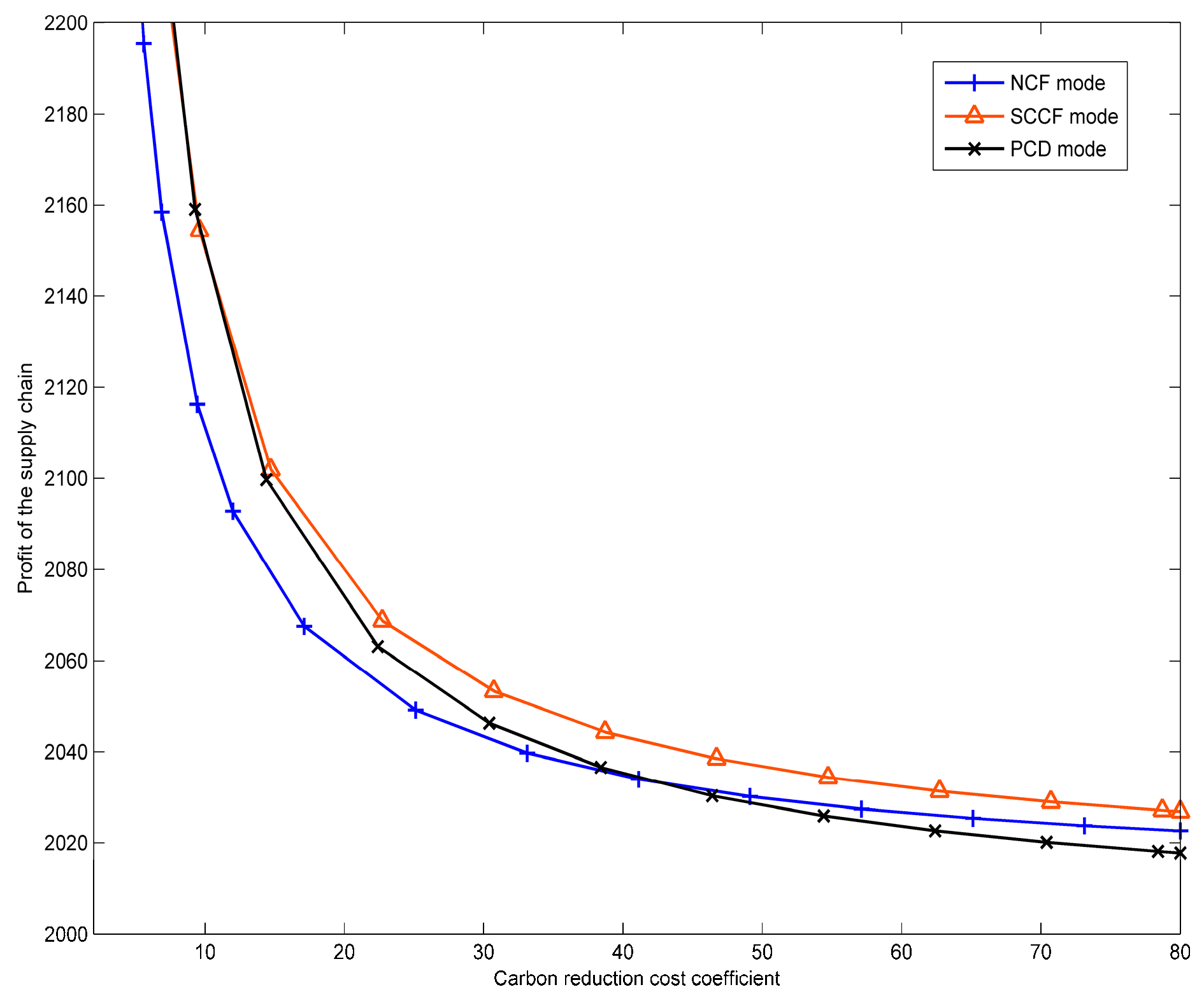
5.2. Impact of on Optimal Profits
6. Conclusions
Acknowledgments
Author Contributions
Conflicts of Interest
Appendix A
A.1. Proof of Lemma 1
A.2. Proof of Lemma 2
A.3. Proof of Lemma 3
A.4. Proof of Lemma 4
A.5. Proof of Theorem 2
A.6. Proof of Theorem 3
A.7. Proof of Theorem 4
A.8. Proofs of Theorems 5 and 6
References
- Guo, W. The Paris Agreement ends free carbon emission era. Energy 2016, 1, 96–99. [Google Scholar]
- Crocker, T.D. The Structuring of Atmospheric Pollution Control Systems; Economics of Air Pollution: New York, NY, USA, 1966; pp. 61–86. [Google Scholar]
- Montgomery, W.D. Markets in licenses and efficient pollution control programs. J. Econ. Theory 1972, 5, 395–418. [Google Scholar] [CrossRef]
- Park, S.J.; Cachon, G.P.; Lai, G.; Seshadri, S. Supply chain design and carbon penalty: Monopoly vs. monopolistic competition. Prod. Oper. Manag. 2015, 24, 1494–1508. [Google Scholar]
- Kameyama, Y.; Morita, K.; Kubota, I. Finance for achieving low-carbon development in Asia: The past, present, and prospects for the future. J. Clean. Prod. 2016, 128, 201–208. [Google Scholar] [CrossRef]
- Hu, X. Potential and challenges of carbon finance development in China. In Proceedings of 2015 2nd International Conference on Industrial Economics System and Industrial Security Engineering; Springer: Singapore, 2016; pp. 367–373. [Google Scholar]
- Cachon, G.P. Retail store density and the cost of greenhouse gas emissions. Manag. Sci. 2014, 60, 1907–1925. [Google Scholar] [CrossRef]
- Purdon, M. Opening the black box of carbon finance “additionality”: The political economy of carbon finance effectiveness across Tanzania, Uganda, and Moldova. World Dev. 2015, 74, 462–478. [Google Scholar] [CrossRef]
- Lee, C.W.; Zhong, J. Financing and risk management of renewable energy projects with a hybrid bond. Renew. Energy 2015, 75, 779–787. [Google Scholar] [CrossRef]
- Yu, X.; Lo, A.Y. Carbon finance and the carbon market in China. Nat. Clim. Chang. 2015, 5, 15–16. [Google Scholar] [CrossRef]
- Modigliani, F.; Miller, M.H. The cost of capital, corporation finance and the theory of investment. Am. Econ. Rev. 1958, 48, 261–297. [Google Scholar]
- Xu, X.; Birge, J.R. Operational decisions, capital structure, and managerial compensation: A news vendor perspective. Eng. Econ. 2008, 53, 173–196. [Google Scholar] [CrossRef]
- Buzacott, J.A.; Zhang, R.Q. Inventory management with asset-based financing. Manag. Technol. 2004, 50, 1274–1292. [Google Scholar] [CrossRef]
- Jing, B.; Chen, X.; Cai, G. Equilibrium financing in a distribution channel with capital constraint. Prod. Oper. Manag. 2012, 21, 1090–1101. [Google Scholar] [CrossRef]
- Cai, G.S.; Chen, X.; Xiao, Z. The roles of bank and trade credits: Theoretical analysis and empirical evidence. Prod. Oper. Manag. 2012, 23, 583–598. [Google Scholar] [CrossRef]
- Yin, Z. The financing problem of SMEs—Implications from the financial supply chain. Res. Financ. Educ. 2014, 2, 6. [Google Scholar]
- Gelsomino, L.M.; Mangiaracina, R.; Perego, A.; Tumino, A. Supply chain finance: A literature review. Int. J. Phys. Distrib. Logist. Manag. 2016, 46, 348–366. [Google Scholar] [CrossRef]
- Wuttke, D.A.; Blome, C.; Foerstl, K.; Henke, M. Managing the innovation adoption of supply chain finance—Empirical evidence from six European case studies. J. Bus. Logist. 2013, 34, 148–166. [Google Scholar] [CrossRef]
- Wuttke, D.A.; Blome, C.; Heese, H.S.; Protopappa-Sieke, M. Supply chain finance: Optimal introduction and adoption decisions. Int. J. Prod. Econ. 2016, 178, 72–81. [Google Scholar] [CrossRef]
- Silvestro, R.; Lustrato, P. Integrating financial and physical supply chains: The role of banks in enabling supply chain integration. Int. J. Oper. Prod. Manag. 2014, 34, 298–324. [Google Scholar] [CrossRef]
- Yan, N.; Dai, H.; Sun, B. Optimal bi-level Stackelberg strategies for supply chain financing with both capital-constrained buyers and sellers. Appl. Stoch. Models Bus. Ind. 2014, 30, 783–796. [Google Scholar] [CrossRef]
- Zhu, Y.; Xie, C.; Sun, B.; Wang, G.J.; Yan, X.G. Predicting China’s SME credit risk in supply chain financing by logistic regression, artificial neural network and hybrid models. Sustainability 2016, 8, 433. [Google Scholar] [CrossRef]
- Li, Y.; Chen, T.; Xin, B. Optimal financing decisions of two cash-constrained supply chains with complementary products. Sustainability 2016, 8, 429. [Google Scholar] [CrossRef]
- Huang, H.; Ke, H.; Wang, L. Equilibrium analysis of pricing competition and cooperation in supply chain with one common manufacturer and duopoly retailers. Int. J. Prod. Econ. 2016, 178, 12–21. [Google Scholar] [CrossRef]
- Yin, S. Alliance formation among perfectly complementary suppliers in a price-sensitive assembly system. Manuf. Ser. Oper. Manag. 2010, 12, 527–544. [Google Scholar] [CrossRef]
- Krishnan, H.; Winter, R.A. Inventory dynamics and supply chain coordination. Manag. Sci. 2010, 56, 141–147. [Google Scholar] [CrossRef]
- Lozano, S.; Moreno, P.; Adenso-Díaz, B.; Algaba, E. Cooperative game theory approach to allocating benefits of horizontal cooperation. Eur. J. Oper. Res. 2013, 229, 444–452. [Google Scholar] [CrossRef]
- Bucki, R.; Suchánek, P. Modelling decision-making processes in the management support of the manufacturing element in the logistic supply chain. Complexity 2017, 2017, 5286135. [Google Scholar] [CrossRef]
- Ma, J.; Lou, W. Complex characteristics of multichannel household appliance supply chain with the price competition. Complexity 2017, 2017, 4327069. [Google Scholar] [CrossRef]
- Almaktoom, A.T. Stochastic reliability measurement and design optimization of an inventory management system. Complexity 2017, 2017, 1460163. [Google Scholar] [CrossRef]
- Gao, J.; Zhang, J. Coordinate the Supply Chain to Reduce Carbon Emissions; LISS 2014; Springer: Berlin/Heidelberg, Germany, 2015; pp. 225–231. [Google Scholar]
- Du, S.; Zhu, J.; Jiao, H.; Ye, W. Game-theoretical analysis for supply chain with consumer preference to low carbon. Int. J. Prod. Res. 2015, 53, 3753–3768. [Google Scholar] [CrossRef]
- Benjaafar, S.; Li, Y.; Daskin, M. Carbon footprint and the management of supply chains: Insights from simple models. IEEE Trans. Autom. Sci. Eng. 2013, 10, 99–116. [Google Scholar] [CrossRef]
- Zhang, C.T.; Liu, L.P. Research on coordination mechanism in three-level green supply chain under non-cooperative game. Appl. Math. Model. 2013, 37, 3369–3379. [Google Scholar] [CrossRef]
- Dales, J.H. Pollution, Property & Prices: An Essay in Policy-Making and Economics; Edward Elgar Publishing: Cheltenham, UK; Northampton, MA, USA, 2002. [Google Scholar]
- Xu, X.; Xu, X.; He, P. Joint production and pricing decisions for multiple products with cap-and-trade and carbon tax regulations. J. Clean. Prod. 2016, 112, 4093–4106. [Google Scholar] [CrossRef]
- Yang, L.; Zheng, C.; Xu, M. Comparisons of low carbon policies in supply chain coordination. J. Syst. Sci. Syst. Eng. 2014, 23, 342–361. [Google Scholar] [CrossRef]
- Drake, D.F.; Kleindorfer, P.R.; Wassenhove, L.N.V. Technology choice and capacity portfolios under emissions regulation. Prod. Oper. Manag. 2016, 25, 1006–1025. [Google Scholar] [CrossRef]
- Carl, J.; Fedor, D. Tracking global carbon revenues: A survey of carbon taxes versus cap-and-trade in the real world. Energy Policy 2016, 96, 50–77. [Google Scholar] [CrossRef]
- Du, S.; Hu, L.; Song, M. Production optimization considering environmental performance and preference in the cap-and-trade system. J. Clean. Prod. 2016, 112, 1600–1607. [Google Scholar] [CrossRef]
- Yang, L.; Ji, J.; Zheng, C. Impact of asymmetric carbon information on supply chain decisions under low-carbon policies. Discret. Dyn. Nat. Soc. 2016, 6, 1–16. [Google Scholar] [CrossRef]
- Wang, Q.P.; Zhao, D.Z.; He, L.F. Contracting emission reduction for supply chains considering market low-carbon preference. J. Clean. Prod. 2016, 120, 72–84. [Google Scholar] [CrossRef]
- Yao, D.; Liu, J. Competitive pricing of mixed retail and e-tail distribution channels. Omega 2005, 33, 235–247. [Google Scholar] [CrossRef]


| Model Parameters | |
|---|---|
| Market scale | |
| Price sensitivity | |
| The unit production cost without including reduction cost | |
| Delay-in-payment | |
| Initial carbon emission of unit product, | |
| Carbon finance | |
| Carbon quota, | |
| Loan amounts of retailer | |
| Carbon reduction cost coefficient | |
| Initial capital | |
| Carbon price, external variable | |
| Production quantity | |
| Interest rate, external variable | |
| Volume of emission trade, | |
| Cost of carbon reduction, | |
| The actual emission, | |
| Non-cooperation | |
| Partial-cooperation | |
| Full-cooperation | |
| Decision variables | |
| Retail price | |
| Wholesale price | |
| The reduction rate of greenhouse gases, | |
| Patterns | Finance | Cooperation | ||
|---|---|---|---|---|
| Delay-in-payment | Bank Loan | Reduction | Price | |
| NCF | × | √ | × | × |
| PCD | √ | × | √ | × |
| SCCF | × | √ | √ | × |
| FC | √ | × | √ | √ |
| Patterns | ||
|---|---|---|
| NCF | ||
| SCCF | ||
| PCD |
| Patterns | ||
|---|---|---|
| NCF | ||
| SCCF | ||
| PCD |
© 2018 by the authors. Licensee MDPI, Basel, Switzerland. This article is an open access article distributed under the terms and conditions of the Creative Commons Attribution (CC BY) license (http://creativecommons.org/licenses/by/4.0/).
Share and Cite
Yang, L.; Chen, Y.; Ji, J. Cooperation Modes of Operations and Financing in a Low-Carbon Supply Chain. Sustainability 2018, 10, 821. https://doi.org/10.3390/su10030821
Yang L, Chen Y, Ji J. Cooperation Modes of Operations and Financing in a Low-Carbon Supply Chain. Sustainability. 2018; 10(3):821. https://doi.org/10.3390/su10030821
Chicago/Turabian StyleYang, Lei, Yufan Chen, and Jingna Ji. 2018. "Cooperation Modes of Operations and Financing in a Low-Carbon Supply Chain" Sustainability 10, no. 3: 821. https://doi.org/10.3390/su10030821
APA StyleYang, L., Chen, Y., & Ji, J. (2018). Cooperation Modes of Operations and Financing in a Low-Carbon Supply Chain. Sustainability, 10(3), 821. https://doi.org/10.3390/su10030821