Forecasting China’s Coal Power Installed Capacity: A Comparison of MGM, ARIMA, GM-ARIMA, and NMGM Models


Abstract
:1. Introduction
2. Literature Review
3. Methodology
3.1. MGM (1,1) Model
3.2. ARIMA Model
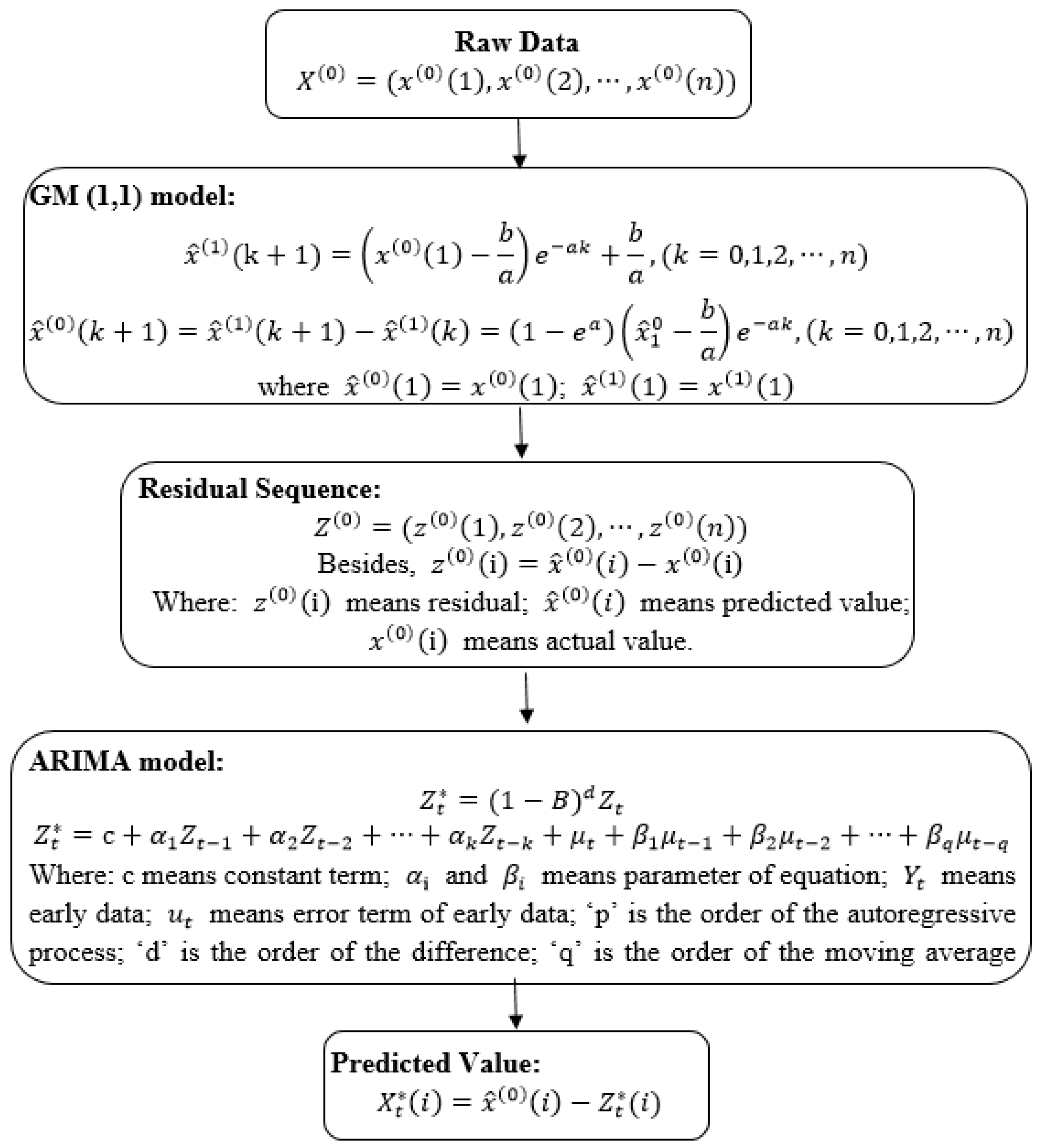
3.3. GM-ARIMA Model
3.4. Non-Linear Metabolic Grey Model
3.5. Measurement of the Forecasting Performance
4. Empirical Results
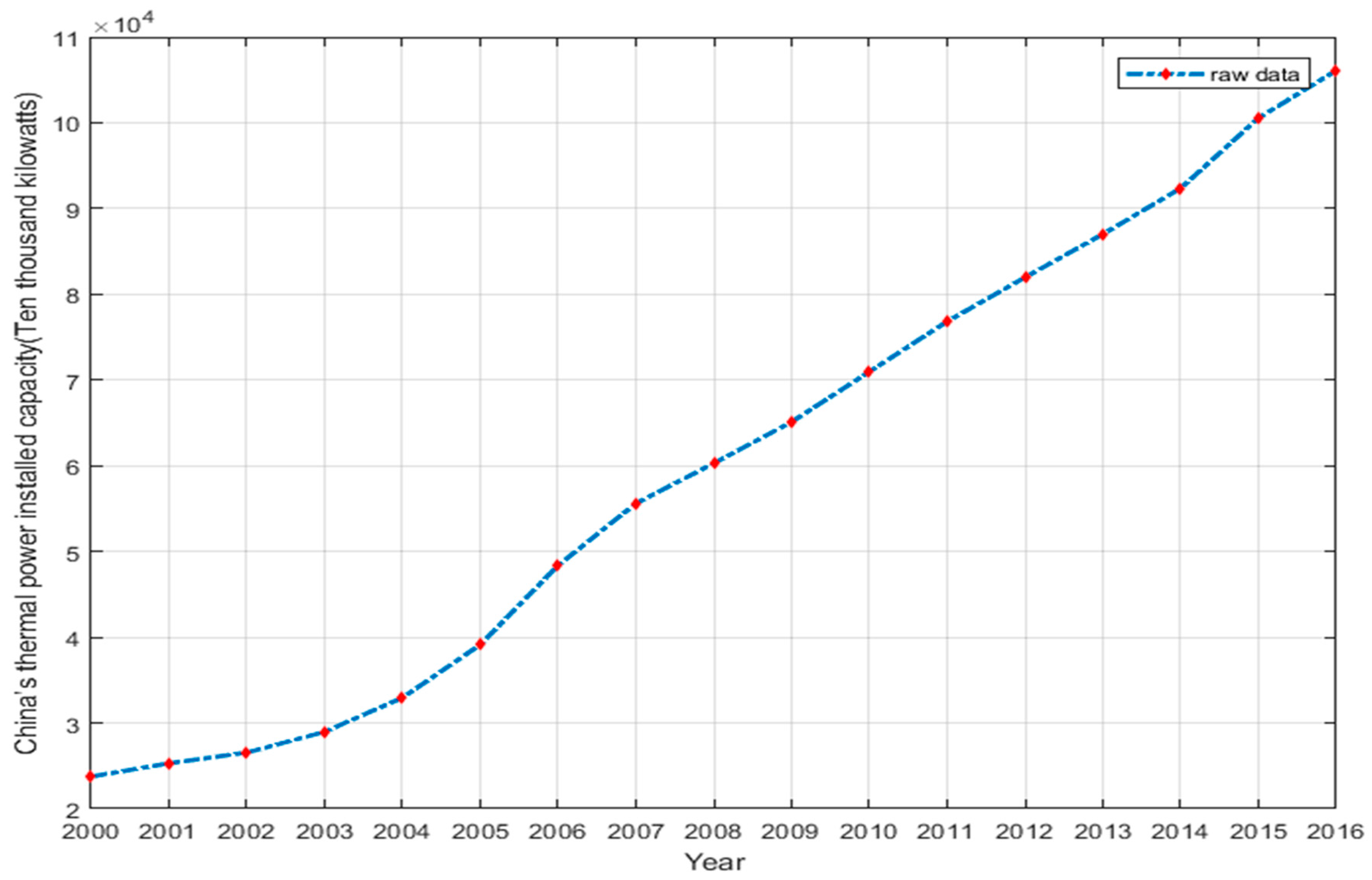
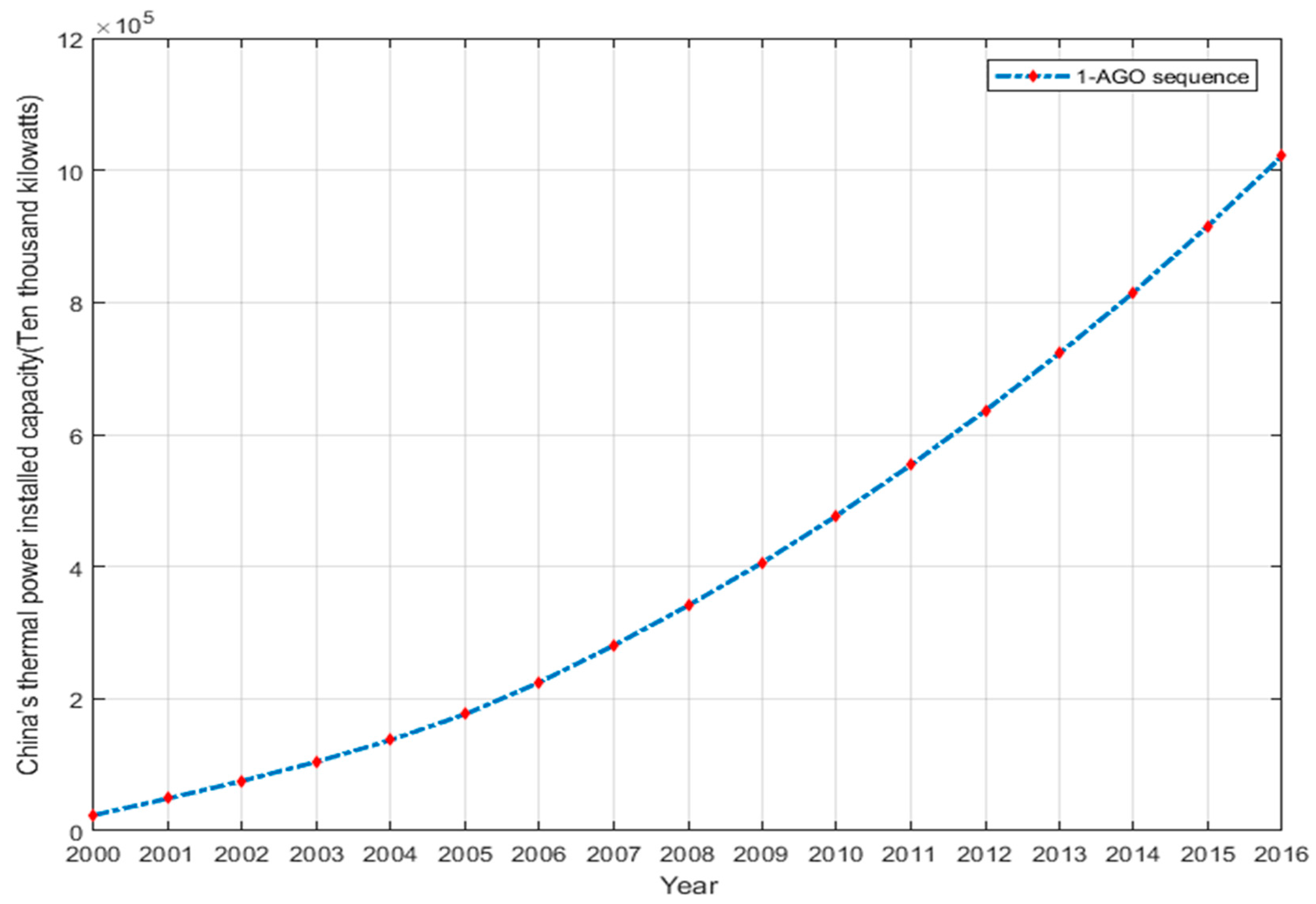
4.1. Display of Thermal Power Capacity
4.2. Linear Parameters
4.3. ARIMA Model Parameters
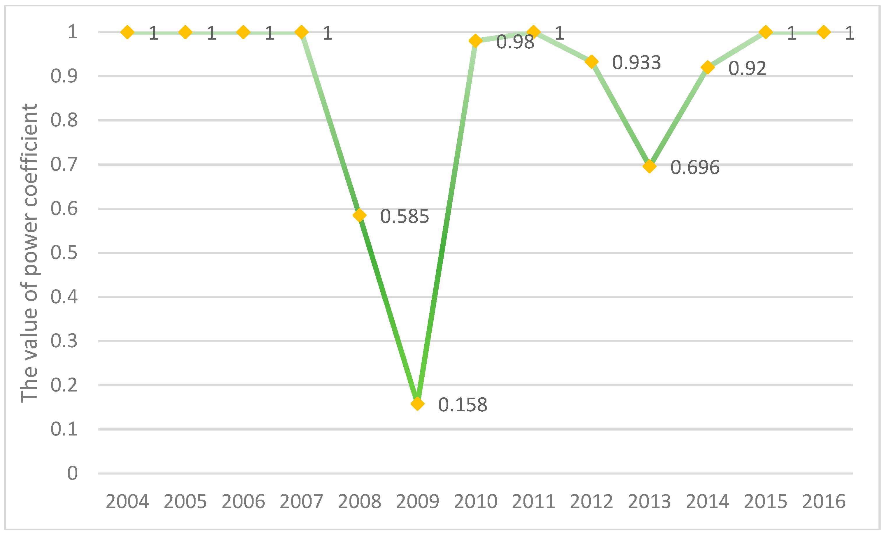
4.4. Nonlinear Parameters
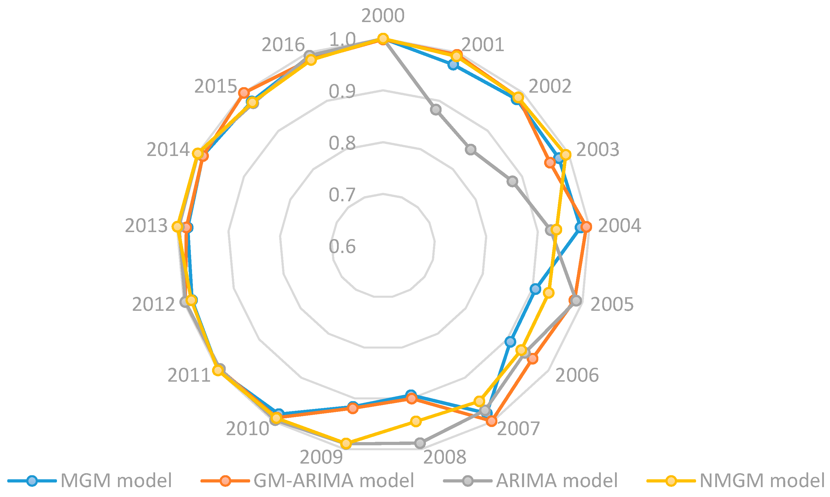
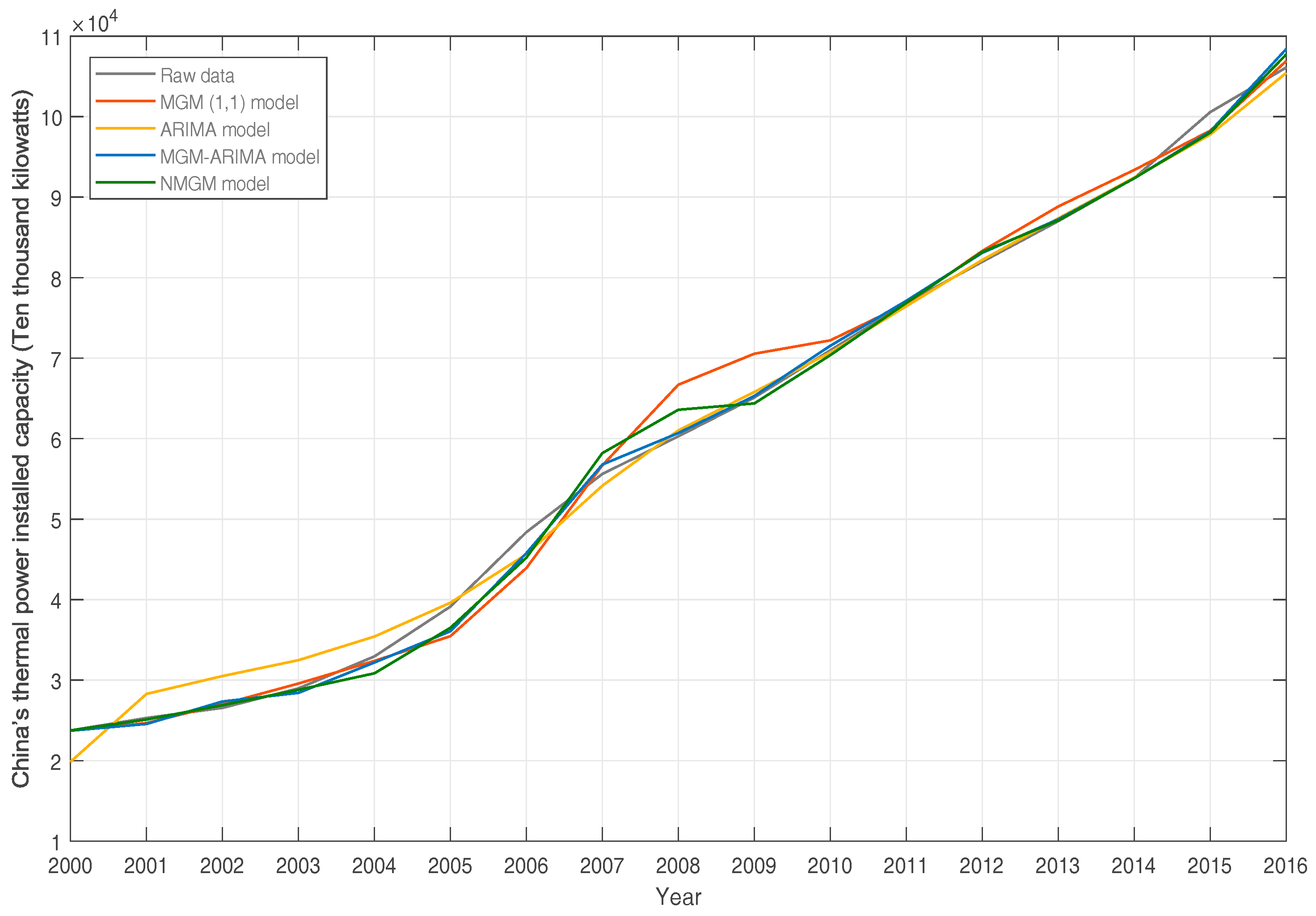
4.5. Comparison and Evaluation of Multiple Models
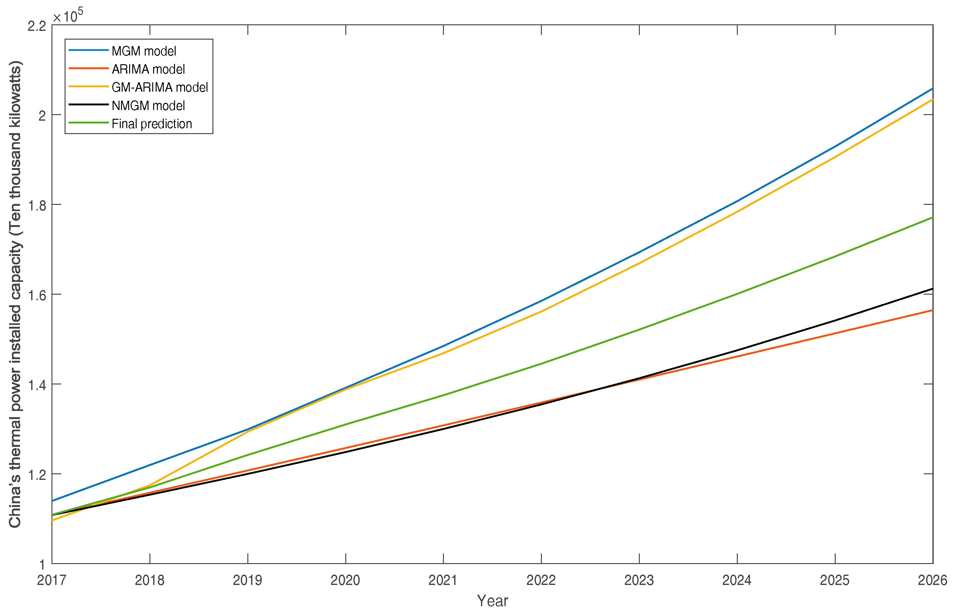
4.6. Forecast Results
5. Conclusions
Acknowledgments
Author Contributions
Conflicts of Interest
References
- Edenhofer, O. King Coal and the queen of subsidies. Science 2015, 349, 1286–1287. [Google Scholar] [CrossRef] [PubMed]
- Wang, Q.; Li, R. Decline in China’s coal consumption: An evidence of peak coal or a temporary blip? Energy Policy 2017, 108, 696–701. [Google Scholar] [CrossRef]
- Peters, G.P.; Andrew, R.M.; Canadell, J.G.; Fuss, S.; Jackson, R.B.; Korsbakken, J.I.; Le Quéré, C.; Nakicenovic, N. Key indicators to track current progress and future ambition of the Paris Agreement. Nat. Clim. Chang. 2017, 7, 118–122. [Google Scholar] [CrossRef]
- Steckel, J.C.; Edenhofer, O.; Jakob, M. Drivers for the renaissance of coal. Proc. Natl. Acad. Sci. USA 2015, 112, E3775–E3781. [Google Scholar] [CrossRef] [PubMed]
- Chu, S.; Majumdar, A. Opportunities and challenges for a sustainable energy future. Nature 2012, 488, 294–303. [Google Scholar] [CrossRef] [PubMed]
- Wang, Q.; Li, R. Journey to burning half of global coal: Trajectory and drivers of China’s coal use. Renew. Sustain. Energy Rev. 2016, 58, 341–346. [Google Scholar] [CrossRef]
- González-Eguino, M.; Olabe, A.; Ribera, T. New coal-fired plants jeopardise Paris agreement. Sustainability 2017, 9, 168. [Google Scholar] [CrossRef]
- Wang, Q.; Chen, X. China’s electricity market-oriented reform: From an absolute to a relative monopoly. Energy Policy 2012, 51, 143–148. [Google Scholar] [CrossRef]
- Wang, Q.; Li, R. Drivers for energy consumption: A comparative analysis of China and India. Renew. Sustain. Energy Rev. 2016, 62, 954–962. [Google Scholar] [CrossRef]
- Zhao, Y.; Wang, S.; Duan, L.; Lei, Y.; Cao, P.; Hao, J. Primary air pollutant emissions of coal-fired power plants in China: Current status and future prediction. Atmos. Environ. 2008, 42, 8442–8452. [Google Scholar] [CrossRef]
- You, C.; Xu, X. Coal combustion and its pollution control in China. Energy 2010, 35, 4467–4472. [Google Scholar] [CrossRef]
- Wang, Q.; Chen, X. Energy policies for managing China’s carbon emission. Renew. Sustain. Energy Rev. 2015, 50, 470–479. [Google Scholar] [CrossRef]
- Zing, N.; Ding, Y.; Pan, J.; Wang, H.; Gregg, J. Climate change-the Chinese challenge. Science 2008, 319, 730–731. [Google Scholar] [CrossRef] [PubMed]
- Wang, Q. Effective policies for renewable energy—The example of China’s wind power—Lessons for China’s photovoltaic power. Renew. Sustain. Energy Rev. 2010, 14, 702–712. [Google Scholar] [CrossRef]
- Biello, D. How much will tar sands oil add to global warming. Sci. Am. 2013, 23, 1–5. [Google Scholar]
- Zhou, L.; Yong, X.L. Electricity Demand Forecasting Based on ARIMA Model and Linear Neural Network. J. Ludong Univ. 2015, 3, 89–94. [Google Scholar]
- Panklib, K.; Prakasvudhisarn, C.; Khummongkol, D. Electricity Consumption Forecasting in Thailand Using an Artificial Neural Network and Multiple Linear Regression. Energy Sources Part B 2015, 10, 427–434. [Google Scholar] [CrossRef]
- Hsu, C.C.; Chen, C.Y. Applications of improved grey prediction model for power demand forecasting. Energy Convers. Manag. 2003, 44, 2241–2249. [Google Scholar] [CrossRef]
- Zhao, H.; Guo, S. An optimized grey model for annual power load forecasting. Energy 2016, 107, 272–286. [Google Scholar] [CrossRef]
- Cui, Z.; Li, L.; Zhao, C.; Yang, T. Traffic Analysis and Forecasting of Power Video Services Based on ARIMA Model. J. Tianjin Univ. 2015, 48, 49–55. [Google Scholar]
- Adhikari, R. A neural network based linear ensemble framework for time series forecasting. Neurocomputing 2015, 157, 231–242. [Google Scholar] [CrossRef]
- Aiello, G.; Cannizzaro, L.; Scalia, G.L.; Muriana, C. An expert system for vineyard management based upon ubiquitous network technologies. Int. J. Serv. Oper. Inform. 2011, 6, 230–247. [Google Scholar] [CrossRef]
- Muriana, C.; Piazza, T.; Vizzini, G. An expert system for financial performance assessment of health care structures based on fuzzy sets and KPIs. Knowl. Based Syst. 2016, 97, 1–10. [Google Scholar] [CrossRef]
- Chen, S.P.; Dang, J.F. A variable spread fuzzy linear regression model with higher explanatory power and forecasting accuracy. Inf. Sci. 2008, 178, 3973–3988. [Google Scholar] [CrossRef]
- D’Urso, P.; Santoro, A. Goodness of fit and variable selection in the fuzzy multiple linear regression. Fuzzy Sets Syst. 2006, 157, 2627–2647. [Google Scholar] [CrossRef]
- Dudek, G. Pattern-based local linear regression models for short-term load forecasting. Electr. Power Syst. Res. 2016, 130, 139–147. [Google Scholar] [CrossRef]
- Sun, H.; Liu, H.; Xiao, H.; He, R.; Ran, B. Use of Local Linear Regression Model for Short-Term Traffic Forecasting. Transp. Res. Rec. J. Transp. Res. Board 2003, 1836, 143–150. [Google Scholar] [CrossRef]
- Shamim, M.A.; Hassan, M.; Ahmad, S.; Zeeshan, M. A comparison of Artificial Neural Networks (ANN) and Local Linear Regression (LLR) techniques for predicting monthly reservoir levels. KSCE J. Civ. Eng. 2016, 20, 971–977. [Google Scholar] [CrossRef]
- Wang, G.; Su, Y.; Shu, L. One-day-ahead daily power forecasting of photovoltaic systems based on partial functional linear regression models. Renew. Energy 2016, 96, 469–478. [Google Scholar] [CrossRef]
- Sun, Y.; Wang, F.; Zhen, Z.; Mi, Z.; Liu, C.; Wang, B.; Lu, J. Research on short-term module temperature prediction model based on BP neural network for photovoltaic power forecasting. In Proceedings of the Power & Energy Society General Meeting, Denver, CO, USA, 26–30 July 2015; pp. 1–5. [Google Scholar]
- Li, J.; Yu, L. Using BP nerual networks for the simulation of energy consumption. In Proceedings of the Institute of Electrical and Electronics Engineers (IEEE) International Conference on Systems, Man and Cybernetics, San Diego, CA, USA, 5–8 October 2014; pp. 3542–3547. [Google Scholar]
- Kang, H.B.; Liu, R.M.; Hou, X.M. Research of power forecasting model of photovoltaic power system based on neural network. Chin. J. Power Sources 2013, 3, 114–116. [Google Scholar]
- Tsekouras, G.J.; Dialynas, E.N.; Hatziargyriou, N.D.; Kavatza, S. A non-linear multivariable regression model for midterm energy forecasting of power systems. Electr. Power Syst. Res. 2007, 77, 1560–1568. [Google Scholar] [CrossRef]
- Kourkoutas, D.; Karanasiou, I.S.; Tsekouras, G.J.; Moshos, M.; Iliakis, E.; Georgopoulos, G. Glaucoma risk assessment using a non-linear multivariable regression method. Comput. Methods Progr. Biomed. 2012, 108, 1149–1159. [Google Scholar] [CrossRef] [PubMed]
- Abushikhah, N.; Elkarmi, F.; Aloquili, O.M. Medium-Term Electric Load Forecasting Using Multivariable Linear and Non-Linear Regression. Smart Grid Renew. Energy 2011, 2, 126–135. [Google Scholar] [CrossRef]
- Wang, Z.X.; Ye, D.J. Forecasting Chinese carbon emissions from fossil energy consumption using non-linear grey multivariable models. J. Clean. Prod. 2017, 142, 600–612. [Google Scholar] [CrossRef]
- Zhong, T.; Guo, W.; Wang, D.; Du, Y. A Novel Nonlinear Grey Bernoulli Forecast Model NGBM(1,1) of Underground Pressure for Working Surface. Electron. J. Geotech. Eng. 2011, 16, 1441–1450. [Google Scholar]
- Ning, Y.; Fan, Y.; Fang, X.; Department, B.E. Water-Saving Irrigation Area of Nonlinear Combination Forecast Based on Grey Model. Henan Sci. 2016, 8, 176–181. [Google Scholar]
- Chen, C.I.; Chen, H.L.; Chen, S.P. Forecasting of foreign exchange rates of Taiwan’s major trading partners by novel nonlinear Grey Bernoulli model NGBM(1, 1). Commun. Nonlinear Sci. Numeri. Simul. 2008, 13, 1194–1204. [Google Scholar] [CrossRef]
- Chen, S.; Jeong, K.; Härdle, W.K. Recurrent support vector regression for a non-linear ARMA model with applications to forecasting financial returns. Comput. Stat. 2015, 30, 821–843. [Google Scholar] [CrossRef]
- Ludlow, J.; Enders, W. Estimating non-linear ARMA models using Fourier coefficients. Int. J. Forecast. 2000, 16, 333–347. [Google Scholar] [CrossRef]
- Deng, J. Grey System Fundamental Method; Huazhong University of Science and Technology: Wuhan, China, 1982. [Google Scholar]
- Wei, L.; Xu, Y.; Chen, C.; Wang, S.; Zhao, R.; Zhang, Y.; Ren, Z. Application of ARIMA Model in Traffic Accident Prediction. J. Beijing Univ. Technol. 2007, 20, 287–288. [Google Scholar]
- Li, S.; Li, R. Comparison of forecasting energy consumption in Shandong, China Using the ARIMA model, GM model, and ARIMA-GM model. Sustainability 2017, 9, 1181. [Google Scholar] [CrossRef]
- Wang, R.; You, Y. Solution of Nonlinear Gompertzlan Gray Model and Its Application. Shopp. Mall Mod. 2017, 17, 19–20. [Google Scholar]
- National Bureau of Statistics of People’s Republic of China (NBSC). China Statistical Yearbook; China Statistical Press: Beijing, China, 2017.


| Notations | Explanation | Notations | Explanation |
|---|---|---|---|
| Original sequence | ‘c’ | Constant term | |
| Once accumulated sequence | , | Harmonic parameter | |
| Prediction of raw sequence | Error term of early data | ||
| Prediction of 1-AGO sequence | Initial data sequence | ||
| B | Matrix of data and constants | Predicted data sequence | |
| Y | Matrix of data | ‘d’ | Order of the difference |
| t | Time sequence | ‘p’ | Order of autoregressive process |
| ‘a’, ‘b’ | Constant parameter | ‘q’ | Order of moving average process |
| Residual sequence | Power coefficient |
| Autocorrelation | Partial Correlation | AC* | PAC** | Q-Stat | Prob | |
|---|---|---|---|---|---|---|
| .|******| | .|******| | 1 | 0.841 | 0.841 | 14.287 | 0.000 |
| .|*****| | .*|.| | 2 | 0.671 | −0.126 | 23.980 | 0.000 |
| .|****| | .*|.| | 3 | 0.503 | −0.094 | 29.809 | 0.000 |
| .|**.| | .*|.| | 4 | 0.332 | −0.121 | 32.547 | 0.000 |
| .|*.| | .*|.| | 5 | 0.164 | −0.117 | 33.272 | 0.000 |
| .|.| | .*|.| | 6 | 0.009 | −0.101 | 33.274 | 0.000 |
| .*|.| | .|.| | 7 | −0.120 | −0.058 | 33.739 | 0.000 |
| .**|.| | .*|.| | 8 | −0.224 | −0.068 | 35.543 | 0.000 |
| .**|.| | .*|.| | 9 | −0.314 | −0.101 | 39.530 | 0.000 |
| .***|.| | .*|.| | 10 | −0.389 | −0.103 | 46.501 | 0.000 |
| .***|.| | .|.| | 11 | −0.431 | −0.049 | 56.514 | 0.000 |
| .***|.| | .|.| | 12 | −0.430 | 0.011 | 68.452 | 0.000 |
| Model | Number of Predictors | Model Fit Statistics | Number of Outliers | |
|---|---|---|---|---|
| Stationary R-Squared | R-Squared | |||
| ARIMA (1,0,0) | 1 | 0.994 | 0.994 | 0 |
| Model | Number of Predictors | Model Fit Statistics | Number of Outliers | |
|---|---|---|---|---|
| Stationary R-Squared | R-Squared | |||
| ARIMA (2,0,1) | 1 | 0.670 | 0.670 | 0 |
| Model 1 | Model 2 | Model 3 | Model 4 | |
|---|---|---|---|---|
| MGM (1,1) | GM-ARIMA | ARIMA (1,0,0) | NMGM (1,1) | |
| MSE | 7,065,216.259 | 4,567,384.561 | 1,908,065.867 | 2,984,472.666 |
| MSPE | 0.002312295 | 0.005201106 | 0.000791596 | 0.001154194 |
| MAPE | 3.37% | 2.13% | 3.71% | 2.36% |
| Year | China’s Thermal Power Installed Capacity/Ten Thousand Kilowatts | Annual Growth Rate |
|---|---|---|
| 2017 | 110,879.2003 | 4.51% |
| 2018 | 116,974.6431 | 5.50% |
| 2019 | 124,207.3304 | 6.18% |
| 2020 | 130,993.5953 | 5.46% |
| 2021 | 137,507.0279 | 4.97% |
| 2022 | 144,522.9155 | 5.10% |
| 2023 | 152,121.2032 | 5.26% |
| 2024 | 160,069.2449 | 5.22% |
| 2025 | 168,409.0602 | 5.21% |
| 2026 | 177,125.3285 | 5.18% |
| 2017 | 110,879.2003 | 5.50% |
© 2018 by the authors. Licensee MDPI, Basel, Switzerland. This article is an open access article distributed under the terms and conditions of the Creative Commons Attribution (CC BY) license (http://creativecommons.org/licenses/by/4.0/).
Share and Cite
Li, S.; Yang, X.; Li, R. Forecasting China’s Coal Power Installed Capacity: A Comparison of MGM, ARIMA, GM-ARIMA, and NMGM Models. Sustainability 2018, 10, 506. https://doi.org/10.3390/su10020506
Li S, Yang X, Li R. Forecasting China’s Coal Power Installed Capacity: A Comparison of MGM, ARIMA, GM-ARIMA, and NMGM Models. Sustainability. 2018; 10(2):506. https://doi.org/10.3390/su10020506
Chicago/Turabian StyleLi, Shuyu, Xue Yang, and Rongrong Li. 2018. "Forecasting China’s Coal Power Installed Capacity: A Comparison of MGM, ARIMA, GM-ARIMA, and NMGM Models" Sustainability 10, no. 2: 506. https://doi.org/10.3390/su10020506
APA StyleLi, S., Yang, X., & Li, R. (2018). Forecasting China’s Coal Power Installed Capacity: A Comparison of MGM, ARIMA, GM-ARIMA, and NMGM Models. Sustainability, 10(2), 506. https://doi.org/10.3390/su10020506