Pattern Matching Trading System Based on the Dynamic Time Warping Algorithm
Abstract
1. Introduction
2. Materials and Methods
2.1. Futures Market
2.2. Dynamic Time Warping
2.3. Pattern Matching Trading System
- -
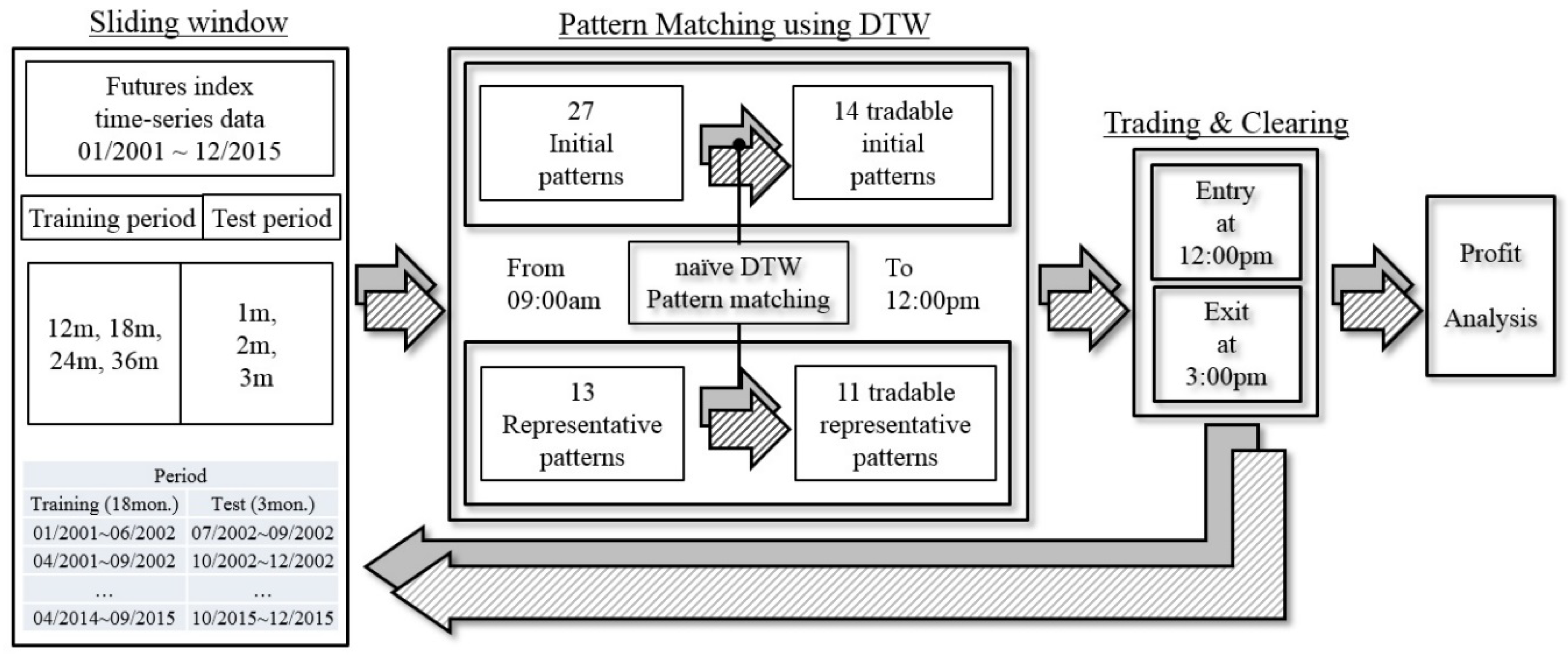
- Enter a long position at 12:00 pm and clear the position by taking a short position at 3:00 pm if the ratio of “up” to “down” for the selected pattern is higher than 1.
- -
- Enter a short position at 12:00 pm and clear the position by taking a long position at 3:00 pm if the ratio of “up” to “down” for the selected pattern is lower than 1.
3. Results
3.1. Data Collection and Preprocessing
3.2. Pattern Matching by the Dynamic Time Warping Algorithm
3.3. Trading Simulation
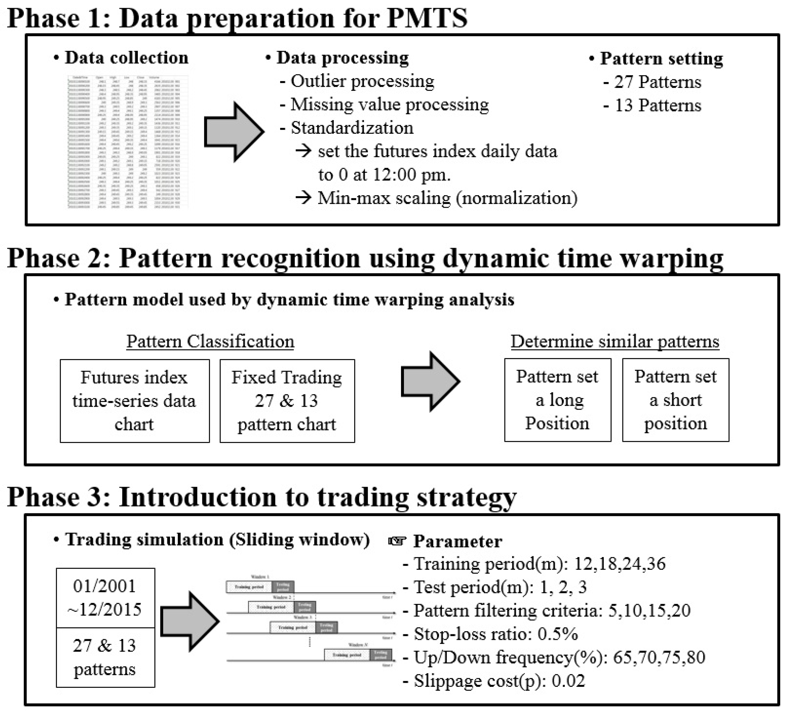
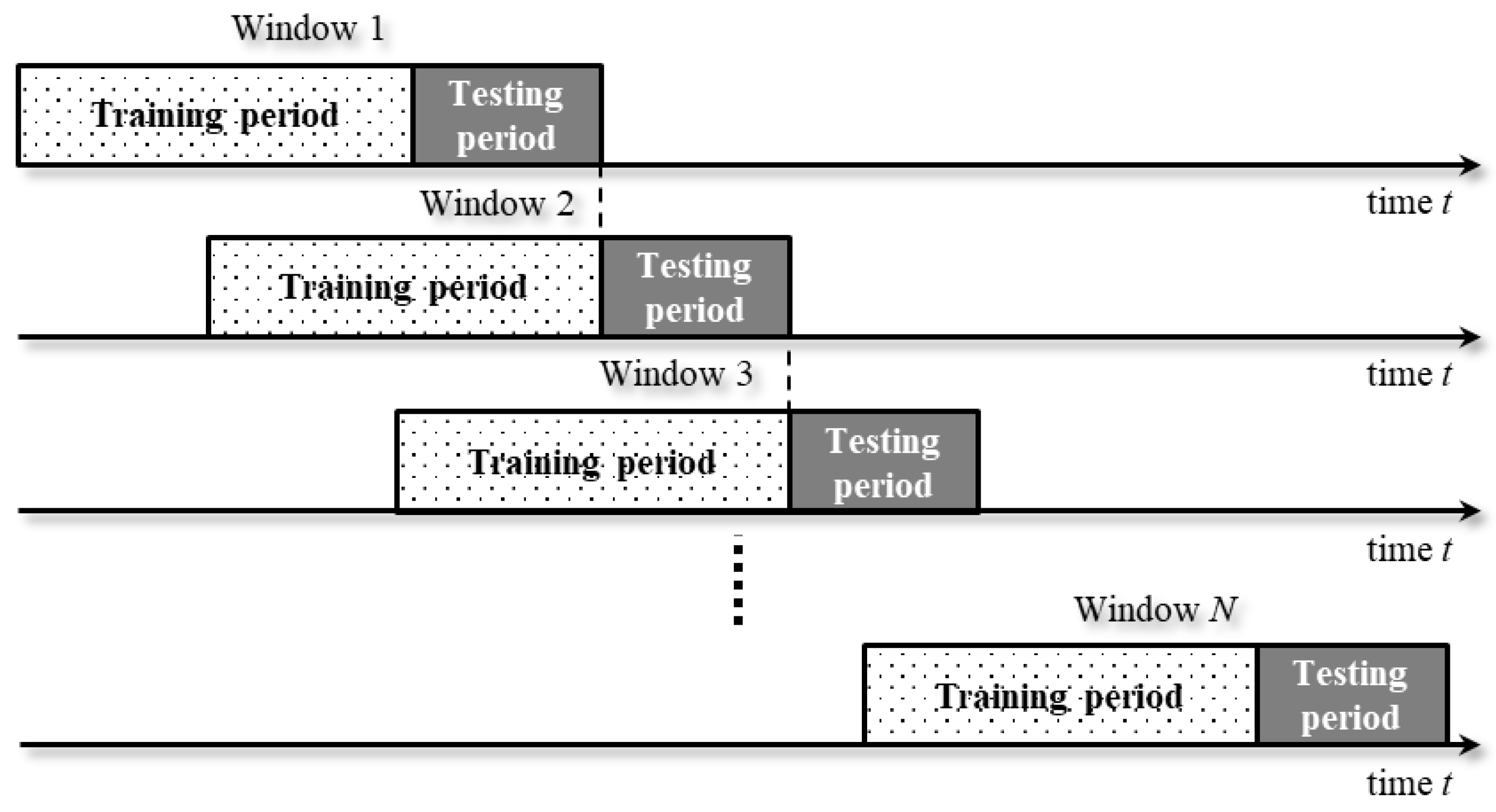
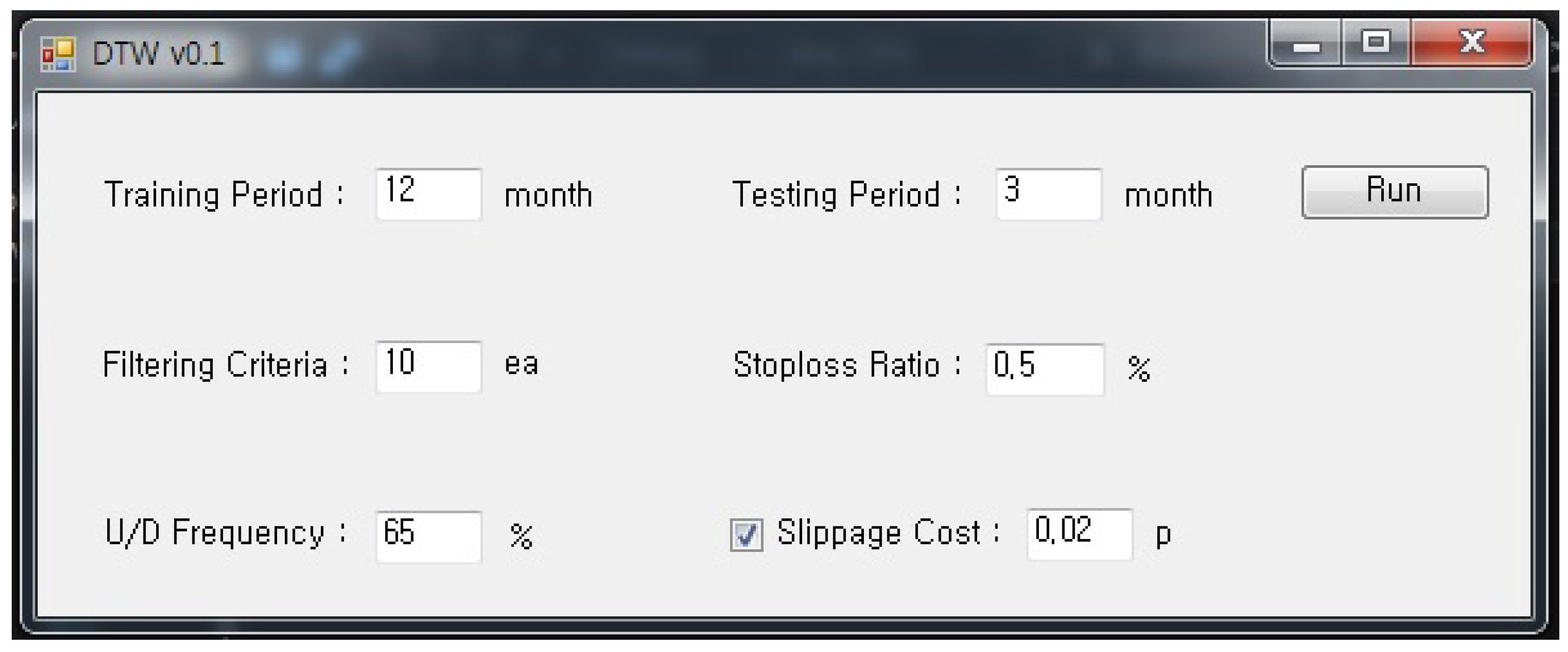
- The training period for pattern matching: 3, 6, 9, 12, 18, 24, 36, 48 and 60 months are used.
- Testing period for trading: 1, 2 and 3 months are used.
- Filtering criteria: a value to exclude patterns if the frequency of a pattern assigned to daily market data is below this value. Seven values of 5, 10, 15, 20, 25, 30 and 40 are used.
- Stop-loss ratio: the rate of loss for the clearing position when the price moves against the predicted direction. 0.5% is used.
- U/D frequency: the proportion of “up” movements in the training period to determine the trading position. Six values of 50%, 60%, 65%, 70%, 75% and 80% are used.
- Slippage cost: the level of slippage cost, where 0.02 pt is used.
3.4. PMTS Results
- -
- Training period: 12, 18, 24 and 36 months
- -
- Testing periods: 1, 2 and 3 months
- -
- Filtering criteria: 5, 10, 15 and 20 ea
- -
- U/D frequency: 65%, 70%, 75% and 80%
4. Discussion
Author Contributions
Conflicts of Interest
References
- Birău, F.R. Financial Derivatives-Meanings beyond Subprime Crisis Stigma. Analele Univ. Constantin Brâncuşi din Târgu Jiu: Ser. Econ. 2010, 2, 195–199. [Google Scholar]
- Carmassi, J.; Gros, D.; Micossi, S. The global financial crisis: Causes and cures. JCMS J. Common Mark. Stud. 2009, 47, 977–996. [Google Scholar] [CrossRef]
- Crotty, J. Structural causes of the global financial crisis: A critical assessment of the ‘new financial architecture’. Camb. J. Econ. 2009, 33, 563–580. [Google Scholar] [CrossRef]
- Ghysels, E.; Seon, J. The Asian financial crisis: The role of derivative securities trading and foreign investors in Korea. J. Int. Money Financ. 2005, 24, 607–630. [Google Scholar] [CrossRef]
- Caillault, É.P.; Lefebvre, A.; Bigand, A. Dynamic time warping-based imputation for univariate time series data. Pattern Recognit. Lett. 2017, in press. [Google Scholar]
- Kwon, D.; Lee, T. Hedging effectiveness of KOSPI200 index futures through VECM-CC-GARCH model. J. Korean Data Inf. Sci. Soc. 2014, 25, 1449–1466. [Google Scholar]
- Keogh, E.J.; Pazzani, M.J. Scaling up dynamic time warping to massive datasets. In European Conference on Principles of Data Mining and Knowledge Discovery; Springer: Berlin/Heidelberg, Germany, 1999; pp. 1–11. [Google Scholar]
- Agrawal, R.; Faloutsos, C.; Swami, A. Efficient similarity search in sequence databases. In International Conference on Foundations of Data Organization and Algorithms; Springer: Berlin/Heidelberg, Germany, 1993; pp. 69–84. [Google Scholar]
- Das, G.; Gunopulos, D.; Mannila, H. Finding similar time series. In European Symposium on Principles of Data Mining and Knowledge Discovery; Springer: Berlin/Heidelberg, Germany, 1997; pp. 88–100. [Google Scholar]
- Fu, T.C.; Chung, F.L.; Luk, R.; Ng, C.M. Stock time series pattern matching: Template-based vs. rule-based approaches. Eng. Appl. Artif. Intell. 2007, 20, 347–364. [Google Scholar] [CrossRef]
- Bagheri, A.; Peyhani, H.M.; Akbari, M. Financial forecasting using ANFIS networks with quantum-behaved particle swarm optimization. Expert Syst. Appl. 2014, 41, 6235–6250. [Google Scholar] [CrossRef]
- Deboeck, G. Trading on the Edge: Neural, Genetic, and Fuzzy Systems for Chaotic Financial Markets; John Wiley & Sons: Hoboken, NJ, USA, 1994; Volume 39. [Google Scholar]
- Leigh, W.; Modani, N.; Hightower, R. A computational implementation of stock charting: Abrupt volume increase as signal for movement in New York stock exchange composite index. Decis. Support Syst. 2004, 37, 515–530. [Google Scholar] [CrossRef]
- Leigh, W.; Modani, N.; Purvis, R.; Roberts, T. Stock market trading rule discovery using technical charting heuristics. Expert Syst. Appl. 2002, 23, 155–159. [Google Scholar] [CrossRef]
- Leigh, W.; Purvis, R.; Ragusa, J.M. Forecasting the NYSE composite index with technical analysis, pattern recognizer, neural network, and genetic algorithm: A case study in romantic decision support. Decis. Support Syst. 2002, 32, 361–377. [Google Scholar] [CrossRef]
- Lo, A.W.; Mamaysky, H.; Wang, J. Foundations of technical analysis: Computational algorithms, statistical inference, and empirical implementation. J. Financ. 2000, 55, 1705–1765. [Google Scholar] [CrossRef]
- Cervelló-Royo, R.; Guijarro, F.; Michniuk, K. Stock market trading rule based on pattern recognition and technical analysis: Forecasting the DJIA index with intraday data. Expert Syst. Appl. 2015, 42, 5963–5975. [Google Scholar] [CrossRef]
- Chen, T.L.; Chen, F.Y. An intelligent pattern recognition model for supporting investment decisions in stock market. Inf. Sci. 2016, 346, 261–274. [Google Scholar] [CrossRef]
- Chung, F.L.; Fu, T.C.; Ng, V.; Luk, R.W. An evolutionary approach to pattern-based time series segmentation. IEEE Trans. Evol. Comput. 2004, 8, 471–489. [Google Scholar] [CrossRef]
- Dong, M.; Zhou, X.S. Exploring the fuzzy nature of technical patterns of US stock market. Proc. Fuzzy Syst. Knowl. Discov. 2002, 1, 324–328. [Google Scholar]
- Kim, S.D.; Lee, J.W.; Lee, J.; Chae, J. A two-phase stock trading system using distributional differences. In International Conference on Database and Expert Systems Applications; Springer: Berlin/Heidelberg, Germany, 2002; pp. 143–152. [Google Scholar]
- Hu, Y.; Feng, B.; Zhang, X.; Ngai, E.W.T.; Liu, M. Stock trading rule discovery with an evolutionary trend following model. Expert Syst. Appl. 2015, 42, 212–222. [Google Scholar] [CrossRef]
- De Oliveira, F.A.; Nobre, C.N.; Zárate, L.E. Applying Artificial Neural Networks to prediction of stock price and improvement of the directional prediction index–Case study of PETR4, Petrobras, Brazil. Expert Syst. Appl. 2013, 40, 7596–7606. [Google Scholar] [CrossRef]
- Patel, J.; Shah, S.; Thakkar, P.; Kotecha, K. Predicting stock and stock price index movement using trend deterministic data preparation and machine learning techniques. Expert Syst. Appl. 2015, 42, 259–268. [Google Scholar] [CrossRef]
- Kahveci, T.; Singh, A.; Gurel, A. Similarity searching for multi-attribute sequences. In Proceedings of the 14th International Conference on Scientific and Statistical Database Management, Edinburgh, UK, 24–26 July 2002; pp. 175–184. [Google Scholar]
- Berndt, D.J.; Clifford, J. Using dynamic time warping to find patterns in time series. KDD Workshop 1994, 10, 359–370. [Google Scholar]
- Senin, P. Dynamic Time Warping Algorithm Review; Information and Computer Science Department University of Hawaii at Manoa Honolulu: Honolulu, HI, USA, 2008; pp. 1–23. [Google Scholar]
- Lee, S.J.; Ahn, J.J.; Oh, K.J.; Kim, T.Y. Using rough set to support investment strategies of real-time trading in futures market. Appl. Intell. 2010, 32, 364–377. [Google Scholar] [CrossRef]
- Lee, S.J.; Oh, K.J.; Kim, T.Y. How many reference patterns can improve profitability for real-time trading in futures market? Expert Syst. Appl. 2012, 39, 7458–7470. [Google Scholar] [CrossRef]
- Tsinaslanidis, P.E. Subsequence dynamic time warping for charting: Bullish and bearish class predictions for NYSE stocks. Expert Syst. Appl. 2018, 94, 193–204. [Google Scholar] [CrossRef]
- Chang, E.C. Returns to speculators and the theory of normal backwardation. J. Financ. 1985, 40, 193–208. [Google Scholar] [CrossRef]
- Hartzmark, M.L. Returns to individual traders of futures: Aggregate results. J. Polit. Econ. 1987, 95, 1292–1306. [Google Scholar] [CrossRef]
- Hartzmark, M.L. Luck versus forecast ability: Determinants of trader performance in futures markets. J. Bus. 1991, 64, 49–74. [Google Scholar] [CrossRef]
- Leuthold, R.M.; Garcia, P.; Lu, R. The returns and forecasting ability of large traders in the frozen pork bellies futures market. J. Bus. 1994, 67, 459–473. [Google Scholar] [CrossRef]
- Wang, C. Investor sentiment and return predictability in agricultural futures markets. J. Futures Mark. Futures Opt. Other Deriv. Prod. 2001, 21, 929–952. [Google Scholar] [CrossRef]
- Bellman, R.; Kalaba, R. On adaptive control processes. IRE Trans. Autom. Control 1959, 4, 1–9. [Google Scholar] [CrossRef]
- Myers, C.; Rabiner, L.; Rosenberg, A. Performance tradeoffs in dynamic time warping algorithms for isolated word recognition. IEEE Trans. Acoust. Speech Signal Process. 1980, 28, 623–635. [Google Scholar] [CrossRef]
- Sakoe, H.; Chiba, S. Dynamic programming algorithm optimization for spoken word recognition. IEEE Trans. Acoust. Speech Signal Process. 1978, 26, 43–49. [Google Scholar] [CrossRef]
- Kuzmanic, A.; Zanchi, V. Hand shape classification using DTW and LCSS as similarity measures for vision-based gesture recognition system. In Proceedings of the International Conference on “Computer as a Tool”, Warsaw, Poland, 9–12 September 2007; pp. 264–269. [Google Scholar]
- Corradini, A. Dynamic time warping for off-line recognition of a small gesture vocabulary. In Proceedings of the Recognition, Analysis, and Tracking of Faces and Gestures in Real-Time Systems, Vancouver, BC, Canada, 13 July 2001; pp. 82–89. [Google Scholar]
- Niennattrakul, V.; Ratanamahatana, C.A. On clustering multimedia time series data using k-means and dynamic time warping. In Proceedings of the 2007 International Conference on Multimedia and Ubiquitous Engineering (MUE’07), Seoul, Korea, 26–28 April 2007; pp. 733–738. [Google Scholar]
- Bahlmann, C.; Burkhardt, H. The writer independent online handwriting recognition system frog on hand and cluster generative statistical dynamic time warping. IEEE Trans. Pattern Anal. Mach. Intell. 2004, 26, 299–310. [Google Scholar] [CrossRef]
- Kahveci, T.; Singh, A. Variable length queries for time series data. In Proceedings of the 17th International Conference on Data Engineering, Heidelberg, Germany, 2–6 April 2001; pp. 273–282. [Google Scholar]
- Müller, M. Dynamic time warping. In Information Retrieval for Music and Motion; Springer: Berlin/Heidelberg, Germany, 2007; pp. 69–84. [Google Scholar]
- Müller, M.; Mattes, H.; Kurth, F. An efficient multiscale approach to audio synchronization. In Proceedings of the 6th International Conference on Music Information Retrieval, London, UK, 11–15 September 2005; pp. 192–197. [Google Scholar]
- Salvador, S.; Chan, P. Toward accurate dynamic time warping in linear time and space. Intell. Data Anal. 2007, 11, 561–580. [Google Scholar] [CrossRef]
- Jang, G.S.; Lai, F.; Jiang, B.W.; Parng, T.M.; Chien, L.H. Intelligent stock trading system with price trend prediction and reversal recognition using dual-module neural networks. Appl. Intell. 1993, 3, 225–248. [Google Scholar] [CrossRef]
- Hwarng, H.B. Insights into neural-network forecasting of time series corresponding to ARMA (p, q) structures. Omega 2001, 29, 273–289. [Google Scholar] [CrossRef]
- Ahn, J.J.; Kim, D.H.; Oh, K.J.; Kim, T.Y. Applying option Greeks to directional forecasting of implied volatility in the options market: An intelligent approach. Expert Syst. Appl. 2012, 39, 9315–9322. [Google Scholar] [CrossRef]
- Ahn, J.J.; Byun, H.W.; Oh, K.J.; Kim, T.Y. Using ridge regression with genetic algorithm to enhance real estate appraisal forecasting. Expert Syst. Appl. 2012, 39, 8369–8379. [Google Scholar] [CrossRef]
- Chou, J.S.; Ngo, N.T. Time series analytics using sliding window metaheuristic optimization-based machine learning system for identifying building energy consumption patterns. Appl. Energy 2016, 177, 751–770. [Google Scholar] [CrossRef]

| Period (mm/yyyy~mm/yyyy) | |||||
|---|---|---|---|---|---|
| Training (18 Months) | Testing (3 Months) | Training (18 Months) | Testing (3 Months) | ||
| Window 1 | 01/2001~06/2002 | 07/2002~09/2002 | Window 28 | 10/2007~03/2009 | 04/2009~06/2009 |
| Window 2 | 04/2001~09/2002 | 10/2002~12/2002 | Window 29 | 01/2008~06/2009 | 07/2009~09/2009 |
| Window 3 | 07/2001~12/2002 | 01/2003~03/2003 | Window 30 | 04/2008~09/2009 | 10/2009~12/2009 |
| Window 4 | 10/2001~03/2003 | 04/2003~06/2003 | Window 31 | 07/2008~12/2009 | 01/2010~03/2010 |
| Window 5 | 01/2002~06/2003 | 07/2003~09/2003 | Window 32 | 10/2008~03/2010 | 04/2010~06/2010 |
| Window 6 | 04/2002~09/2003 | 10/2003~12/2003 | Window 33 | 01/2009~06/2010 | 07/2010~09/2010 |
| Window 7 | 07/2002~12/2003 | 01/2004~03/2004 | Window 34 | 04/2009~09/2010 | 10/2010~12/2010 |
| Window 8 | 10/2002~03/2004 | 04/2004~06/2004 | Window 35 | 07/2009~12/2010 | 01/2011~03/2011 |
| Window 9 | 01/2003~06/2004 | 07/2004~09/2004 | Window 36 | 10/2009~03/2011 | 04/2011~06/2011 |
| Window 10 | 04/2003~09/2004 | 10/2004~12/2004 | Window 37 | 01/2010~06/2011 | 07/2011~09/2011 |
| Window 11 | 07/2003~12/2004 | 01/2005~03/2005 | Window 38 | 04/2010~09/2011 | 10/2011~12/2011 |
| Window 12 | 10/2003~03/2005 | 04/2005~06/2005 | Window 39 | 07/2010~12/2011 | 01/2012~03/2012 |
| Window 13 | 01/2004~06/2005 | 07/2005~09/2005 | Window 40 | 10/2010~03/2012 | 04/2012~06/2012 |
| Window 14 | 04/2004~09/2005 | 10/2005~12/2005 | Window 41 | 01/2011~06/2012 | 07/2012~09/2012 |
| Window 15 | 07/2004~12/2005 | 01/2006~03/2006 | Window 42 | 04/2011~09/2012 | 10/2012~12/2012 |
| Window 16 | 10/2004~03/2006 | 04/2006~06/2006 | Window 43 | 07/2011~12/2012 | 01/2013~03/2013 |
| Window 17 | 01/2005~06/2006 | 07/2006~09/2006 | Window 44 | 10/2011~03/2013 | 04/2013~06/2013 |
| Window 18 | 04/2005~09/2006 | 10/2006~12/2006 | Window 45 | 01/2012~06/2013 | 07/2013~09/2013 |
| Window 19 | 07/2005~12/2006 | 01/2007~03/2007 | Window 46 | 04/2012~09/2013 | 10/2013~12/2013 |
| Window 20 | 10/2005~03/2007 | 04/2007~06/2007 | Window 47 | 07/2012~12/2013 | 01/2014~03/2014 |
| Window 21 | 01/2006~06/2007 | 07/2007~09/2007 | Window 48 | 10/2012~03/2014 | 04/2014~06/2014 |
| Window 22 | 04/2006~09/2007 | 10/2007~12/2007 | Window 49 | 01/2013~06/2014 | 07/2014~09/2014 |
| Window 23 | 07/2006~12/2007 | 01/2008~03/2008 | Window 50 | 04/2013~09/2014 | 10/2014~12/2014 |
| Window 24 | 10/2006~03/2008 | 04/2008~06/2008 | Window 51 | 07/2013~12/2014 | 01/2015~03/2015 |
| Window 25 | 01/2007~06/2008 | 07/2008~09/2008 | Window 52 | 10/2013~03/2015 | 04/2015~06/2015 |
| Window 26 | 04/2007~09/2008 | 10/2008~12/2008 | Window 53 | 01/2014~06/2015 | 07/2015~09/2015 |
| Window 27 | 07/2007~12/2008 | 01/2009~03/2009 | Window 54 | 04/2014~09/2015 | 10/2015~12/2015 |
| Training Period | |||||
|---|---|---|---|---|---|
| Month | 12 | 18 | 24 | 36 | |
| Testing Period | 1 | 168 | 162 | 156 | 144 |
| 2 | 84 | 81 | 78 | 72 | |
| 3 | 56 | 54 | 52 | 48 | |
| Representative Pattern (rp) | |||||||||||||
|---|---|---|---|---|---|---|---|---|---|---|---|---|---|
| 1 | 2 | 3 | 4 | 5 | 6 | 7 | 8 | 9 | 10 | 11 | 12 | 13 | |
| Window 1 | 44 | 61 | 8 | 10 | 7 | 12 | 8 | 18 | 78 | 73 | 8 | 9 | 29 |
| Window 2 | 47 | 55 | 6 | 9 | 5 | 12 | 10 | 15 | 85 | 74 | 8 | 7 | 34 |
| Window 3 | 50 | 55 | 6 | 11 | 5 | 15 | 13 | 14 | 91 | 61 | 6 | 5 | 35 |
| Window 4 | 52 | 57 | 5 | 10 | 6 | 18 | 13 | 13 | 89 | 56 | 4 | 6 | 38 |
| Window 5 | 49 | 59 | 5 | 8 | 6 | 20 | 11 | 11 | 95 | 54 | 3 | 5 | 41 |
| Window 6 | 54 | 56 | 4 | 10 | 7 | 17 | 11 | 12 | 93 | 53 | 2 | 6 | 44 |
| Window 7 | 57 | 52 | 7 | 9 | 9 | 14 | 12 | 13 | 102 | 49 | 2 | 5 | 40 |
| Window 8 | 62 | 56 | 8 | 8 | 9 | 14 | 12 | 15 | 99 | 46 | 3 | 4 | 33 |
| Window 9 | 54 | 57 | 8 | 6 | 11 | 13 | 8 | 18 | 99 | 57 | 2 | 4 | 31 |
| Window 10 | 52 | 58 | 9 | 5 | 11 | 11 | 8 | 22 | 110 | 53 | 3 | 4 | 23 |
| Window 11 | 48 | 61 | 10 | 4 | 9 | 12 | 8 | 24 | 107 | 60 | 3 | 7 | 20 |
| Window 12 | 45 | 64 | 9 | 3 | 9 | 15 | 8 | 22 | 108 | 58 | 7 | 9 | 15 |
| Window 13 | 38 | 68 | 8 | 5 | 8 | 17 | 5 | 20 | 105 | 62 | 9 | 9 | 17 |
| Window 14 | 34 | 67 | 7 | 6 | 10 | 22 | 5 | 18 | 110 | 61 | 8 | 9 | 18 |
| Window 15 | 40 | 69 | 7 | 6 | 11 | 22 | 6 | 18 | 107 | 55 | 9 | 9 | 18 |
| Window 16 | 41 | 73 | 7 | 8 | 9 | 24 | 6 | 14 | 104 | 55 | 8 | 9 | 19 |
| Window 17 | 40 | 70 | 5 | 10 | 10 | 22 | 7 | 12 | 108 | 52 | 8 | 6 | 23 |
| Window 18 | 41 | 74 | 7 | 9 | 9 | 22 | 10 | 13 | 101 | 51 | 6 | 4 | 29 |
| Window 19 | 39 | 74 | 6 | 10 | 12 | 24 | 12 | 10 | 102 | 48 | 4 | 4 | 29 |
| Window 20 | 37 | 77 | 7 | 11 | 13 | 17 | 13 | 10 | 96 | 50 | 4 | 3 | 34 |
| Window 21 | 39 | 75 | 8 | 11 | 12 | 18 | 14 | 10 | 102 | 43 | 4 | 3 | 32 |
| Window 22 | 41 | 71 | 7 | 10 | 15 | 18 | 14 | 10 | 99 | 39 | 7 | 3 | 34 |
| Window 23 | 44 | 67 | 9 | 8 | 16 | 20 | 14 | 10 | 96 | 41 | 9 | 3 | 32 |
| Window 24 | 43 | 62 | 11 | 10 | 14 | 17 | 13 | 11 | 99 | 43 | 9 | 5 | 30 |
| Window 25 | 48 | 59 | 10 | 9 | 16 | 13 | 12 | 15 | 93 | 47 | 10 | 6 | 29 |
| Window 26 | 49 | 55 | 9 | 7 | 14 | 16 | 10 | 16 | 94 | 47 | 10 | 9 | 33 |
| Window 27 | 42 | 53 | 9 | 7 | 15 | 15 | 9 | 14 | 92 | 57 | 11 | 8 | 38 |
| Window 28 | 40 | 55 | 8 | 5 | 13 | 12 | 11 | 18 | 98 | 57 | 9 | 7 | 38 |
| Window 29 | 38 | 59 | 7 | 5 | 15 | 8 | 11 | 19 | 98 | 54 | 11 | 8 | 39 |
| Window 30 | 39 | 67 | 7 | 3 | 16 | 8 | 11 | 20 | 98 | 55 | 11 | 6 | 36 |
| Window 31 | 37 | 71 | 7 | 3 | 10 | 9 | 12 | 22 | 100 | 56 | 12 | 6 | 35 |
| Window 32 | 39 | 73 | 7 | 3 | 11 | 9 | 13 | 25 | 102 | 50 | 12 | 6 | 27 |
| Window 33 | 43 | 73 | 8 | 3 | 8 | 10 | 12 | 27 | 97 | 50 | 13 | 7 | 25 |
| Window 34 | 47 | 69 | 9 | 4 | 8 | 13 | 12 | 24 | 95 | 55 | 13 | 8 | 21 |
| Window 35 | 50 | 66 | 9 | 7 | 5 | 17 | 11 | 23 | 94 | 59 | 13 | 9 | 17 |
| Window 36 | 52 | 59 | 7 | 8 | 5 | 17 | 10 | 19 | 101 | 56 | 11 | 9 | 20 |
| Window 37 | 52 | 52 | 9 | 7 | 6 | 16 | 10 | 14 | 110 | 53 | 10 | 10 | 24 |
| Window 38 | 51 | 49 | 13 | 7 | 4 | 15 | 8 | 11 | 113 | 59 | 11 | 7 | 27 |
| Window 39 | 54 | 48 | 11 | 7 | 4 | 17 | 10 | 11 | 114 | 59 | 8 | 7 | 26 |
| Window 40 | 51 | 50 | 12 | 6 | 4 | 16 | 10 | 10 | 113 | 60 | 7 | 7 | 29 |
| Window 41 | 49 | 48 | 11 | 7 | 4 | 14 | 12 | 11 | 109 | 57 | 3 | 5 | 41 |
| Window 42 | 46 | 52 | 10 | 8 | 4 | 17 | 12 | 11 | 105 | 57 | 5 | 6 | 42 |
| Window 43 | 53 | 53 | 10 | 8 | 5 | 21 | 10 | 12 | 95 | 57 | 6 | 4 | 40 |
| Window 44 | 48 | 56 | 7 | 9 | 8 | 20 | 12 | 15 | 94 | 57 | 5 | 4 | 37 |
| Window 45 | 38 | 56 | 7 | 9 | 10 | 18 | 12 | 13 | 103 | 54 | 6 | 4 | 41 |
| Window 46 | 34 | 62 | 5 | 9 | 9 | 21 | 10 | 15 | 102 | 52 | 9 | 4 | 39 |
| Window 47 | 32 | 69 | 5 | 5 | 8 | 23 | 7 | 15 | 111 | 53 | 9 | 5 | 30 |
| Window 48 | 31 | 67 | 5 | 3 | 9 | 24 | 8 | 18 | 107 | 57 | 7 | 4 | 29 |
| Window 49 | 23 | 72 | 5 | 3 | 8 | 24 | 9 | 17 | 113 | 53 | 6 | 6 | 29 |
| Window 50 | 26 | 72 | 4 | 4 | 7 | 27 | 6 | 16 | 113 | 52 | 5 | 7 | 30 |
| Window 51 | 31 | 71 | 3 | 4 | 6 | 29 | 7 | 17 | 102 | 56 | 9 | 8 | 26 |
| Window 52 | 32 | 72 | 5 | 4 | 7 | 27 | 7 | 15 | 100 | 55 | 6 | 7 | 30 |
| Window 53 | 38 | 62 | 7 | 6 | 8 | 28 | 7 | 15 | 97 | 54 | 6 | 9 | 30 |
| Window 54 | 36 | 58 | 10 | 6 | 7 | 25 | 5 | 16 | 102 | 52 | 7 | 8 | 37 |
| Clearing Time | ||||||||
|---|---|---|---|---|---|---|---|---|
| 14:00 | 14:10 | 14:20 | 14:30 | 14:40 | 14:50 | 15:00 | ||
| rp-1 | U | 25 | 22 | 22 | 23 | 21 | 26 | 28 |
| D | 19 | 22 | 22 | 21 | 23 | 18 | 16 | |
| UD | U | U | U | U | D | U | U | |
| rp-2 | U | 26 | 28 | 25 | 26 | 28 | 29 | 28 |
| D | 35 | 33 | 36 | 35 | 33 | 32 | 33 | |
| UD | D | D | D | D | D | D | D | |
| rp-9 | U | 38 | 40 | 40 | 39 | 41 | 39 | 42 |
| D | 40 | 38 | 38 | 39 | 37 | 39 | 35 | |
| UD | D | U | U | U | U | U | U | |
| rp-10 | U | 39 | 47 | 39 | 38 | 36 | 36 | 32 |
| D | 34 | 26 | 34 | 35 | 37 | 37 | 41 | |
| UD | U | U | U | U | D | D | D | |
| rp-13 | U | 10 | 9 | 9 | 10 | 10 | 11 | 8 |
| D | 19 | 20 | 20 | 19 | 19 | 18 | 20 | |
| UD | D | D | D | D | D | D | D | |
| Clearing Time | ||||||||
|---|---|---|---|---|---|---|---|---|
| 14:00 | 14:10 | 14:20 | 14:30 | 14:40 | 14:50 | 15:00 | ||
| rp-1 | U | 25 | 22 | 22 | 23 | 21 | 26 | 28 |
| D | 19 | 22 | 22 | 21 | 23 | 18 | 16 | |
| UD | M | M | M | M | M | M | M | |
| rp-2 | U | 26 | 28 | 25 | 26 | 28 | 29 | 28 |
| D | 35 | 33 | 36 | 35 | 33 | 32 | 33 | |
| UD | M | M | M | M | M | M | M | |
| rp-9 | U | 38 | 40 | 40 | 39 | 41 | 39 | 42 |
| D | 40 | 38 | 38 | 39 | 37 | 39 | 35 | |
| UD | M | M | M | M | M | M | M | |
| rp-10 | U | 39 | 47 | 39 | 38 | 36 | 36 | 32 |
| D | 34 | 26 | 34 | 35 | 37 | 37 | 41 | |
| UD | M | M | M | M | M | M | M | |
| rp-13 | U | 10 | 9 | 9 | 10 | 10 | 11 | 8 |
| D | 19 | 20 | 20 | 19 | 19 | 18 | 20 | |
| UD | D | D | D | D | D | M | D | |
| Performance | (Training Period, Testing Period) | |||||||||||
|---|---|---|---|---|---|---|---|---|---|---|---|---|
| (12,1) | (12,2) | (12,3) | (18,1) | (18,2) | (18,3) | (24,1) | (24,2) | (24,3) | (36,1) | (36,2) | (36,3) | |
| Annualized return | 16.62 | 16.45 | 18.48 | 19.59 | 16.99 | 19.17 | 18.13 | 18.67 | 19.38 | 17.81 | 16.50 | 18.43 |
| StDev | 31.32 | 22.91 | 21.49 | 30.63 | 23.10 | 18.83 | 29.27 | 22.10 | 20.88 | 31.42 | 23.88 | 21.72 |
| Sharpe ratio | 0.48 | 0.65 | 0.79 | 0.59 | 0.67 | 0.94 | 0.57 | 0.78 | 0.86 | 0.52 | 0.63 | 0.78 |
| Performance | (Filtering Criteria, Up/Down Frequency (%)) | |||||||||||||||
|---|---|---|---|---|---|---|---|---|---|---|---|---|---|---|---|---|
| (5,65) | (5,70) | (5,75) | (5,80) | (10,65) | (10,70) | (10,75) | (10,80) | (15,65) | (15,70) | (15,75) | (15,80) | (20,65) | (20,70) | (20,75) | (20,80) | |
| Annualized return | 18.83 | 1.30 | 0.63 | 0.69 | 18.27 | 0.91 | 0.12 | 0.32 | 19.17 | 0.69 | 0.06 | 0.09 | 19.17 | 0.25 | −0.03 | 0.00 |
| StDev | 18.63 | 4.59 | 2.64 | 2.26 | 19.18 | 4.37 | 1.87 | 1.67 | 19.53 | 3.63 | 0.70 | 0.65 | 18.83 | 3.29 | 0.23 | 0.00 |
| Sharpe ratio | 0.93 | −0.04 | −0.33 | −0.36 | 0.87 | −0.14 | −0.74 | −0.71 | 0.90 | −0.22 | −2.07 | −2.16 | 0.94 | −0.38 | −6.53 | 0.00 |
| Performance | (Training Period, Testing Period) | |||||||||||
|---|---|---|---|---|---|---|---|---|---|---|---|---|
| (12,1) | (12,2) | (12,3) | (18,1) | (18,2) | (18,3) | (24,1) | (24,2) | (24,3) | (36,1) | (36,2) | (36,3) | |
| Annualized return | 17.20 | 16.91 | 17.81 | 17.26 | 16.06 | 16.50 | 18.42 | 18.65 | 18.66 | 18.63 | 18.03 | 18.48 |
| StDev | 36.36 | 26.92 | 25.86 | 33.21 | 26.40 | 22.65 | 31.87 | 25.11 | 22.68 | 34.39 | 26.76 | 23.87 |
| Sharpe ratio | 0.43 | 0.57 | 0.63 | 0.47 | 0.55 | 0.66 | 0.53 | 0.68 | 0.76 | 0.50 | 0.62 | 0.71 |
| Performance | (Filtering Criteria, Up/Down Frequency (%)) | |||||||||||||||
|---|---|---|---|---|---|---|---|---|---|---|---|---|---|---|---|---|
| (5,65) | (5,70) | (5,75) | (5,80) | (10,65) | (10,70) | (10,75) | (10,80) | (15,65) | (15,70) | (15,75) | (15,80) | (20,65) | (20,70) | (20,75) | (20,80) | |
| Annualized return | 18.54 | 1.26 | 0.25 | 0.09 | 18.66 | 1.09 | 0.01 | −0.11 | 17.80 | 0.99 | −0.01 | 0.00 | 18.25 | 1.20 | −0.03 | 0.00 |
| StDev | 21.78 | 4.92 | 2.59 | 2.04 | 22.68 | 4.10 | 1.70 | 0.90 | 22.51 | 3.67 | 1.07 | 0.00 | 22.91 | 3.88 | 1.01 | 0.00 |
| Sharpe ratio | 0.78 | −0.05 | −0.48 | −0.69 | 0.76 | −0.10 | −0.88 | −1.79 | 0.72 | −0.14 | −1.42 | 0.00 | 0.73 | −0.08 | −1.52 | 0.00 |
| Trading Exit Time | 14:00 | 14:10 | 14:20 | 14:30 | 14:40 | 14:50 | 15:00 | Avg. |
|---|---|---|---|---|---|---|---|---|
| Annualized return | 7.24 (0.0153) | 11.42 (0.0002) | 13.07 (0.0000) | 13.80 (0.0000) | 17.65 (0.0000) | 18.05 (0.0000) | 19.17 (0.0000) | 14.34 |
| StDev | 21.05 | 20.41 | 18.78 | 21.33 | 23.15 | 24.61 | 18.83 | 21.17 |
| Sharpe Ratio | 0.27 | 0.49 | 0.62 | 0.58 | 0.70 | 0.67 | 0.94 | 0.61 |
| Trading Exit Time | 14:00 | 14:10 | 14:20 | 14:30 | 14:40 | 14:50 | 15:00 | Avg. |
|---|---|---|---|---|---|---|---|---|
| Annualized return | 7.25 (0.0098) | 10.93 (0.0004) | 12.72 (0.0002) | 13.39 (0.0000) | 15.52 (0.0000) | 17.64 (0.0000) | 18.66 (0.0000) | 13.73 |
| StDev | 19.31 | 20.40 | 22.88 | 19.18 | 22.13 | 23.40 | 22.68 | 21.43 |
| Sharpe Ratio | 0.30 | 0.46 | 0.49 | 0.62 | 0.63 | 0.69 | 0.76 | 0.56 |
| Avg. of Total Profit (pt) | 14:00 | 14:10 | 14:20 | 14:30 | 14:40 | 14:50 | 15:00 | Avg. |
|---|---|---|---|---|---|---|---|---|
| 13 pattern 1 | 3.62 (0.0153) | 5.71 (0.0002) | 6.53 (0.0000) | 6.90 (0.0000) | 8.83 (0.0000) | 9.02 (0.0000) | 9.58 (0.0000) | 7.17 |
| 27 pattern 2 | 3.63 (0.0098) | 5.46 (0.0004) | 6.36 (0.0002) | 6.69 (0.0000) | 7.76 (0.0000) | 8.82 (0.0000) | 9.33 (0.0000) | 6.87 |
© 2018 by the authors. Licensee MDPI, Basel, Switzerland. This article is an open access article distributed under the terms and conditions of the Creative Commons Attribution (CC BY) license (http://creativecommons.org/licenses/by/4.0/).
Share and Cite
Kim, S.H.; Lee, H.S.; Ko, H.J.; Jeong, S.H.; Byun, H.W.; Oh, K.J. Pattern Matching Trading System Based on the Dynamic Time Warping Algorithm. Sustainability 2018, 10, 4641. https://doi.org/10.3390/su10124641
Kim SH, Lee HS, Ko HJ, Jeong SH, Byun HW, Oh KJ. Pattern Matching Trading System Based on the Dynamic Time Warping Algorithm. Sustainability. 2018; 10(12):4641. https://doi.org/10.3390/su10124641
Chicago/Turabian StyleKim, Sang Hyuk, Hee Soo Lee, Han Jun Ko, Seung Hwan Jeong, Hyun Woo Byun, and Kyong Joo Oh. 2018. "Pattern Matching Trading System Based on the Dynamic Time Warping Algorithm" Sustainability 10, no. 12: 4641. https://doi.org/10.3390/su10124641
APA StyleKim, S. H., Lee, H. S., Ko, H. J., Jeong, S. H., Byun, H. W., & Oh, K. J. (2018). Pattern Matching Trading System Based on the Dynamic Time Warping Algorithm. Sustainability, 10(12), 4641. https://doi.org/10.3390/su10124641


