Is It Correct to Use the Internal Rate of Return to Evaluate the Sustainability of Investment Decisions in Public Private Partnership Projects?

Abstract

Public Private Partnerships (PPP) are viewed by the private sector as investment projects. An investment criterion, such as the internal rate of return (IRR), widely used by practitioners, is thus necessary in order to determine if the opportunity is sustainable from an economic point of view and worth pursuing. However, a cash flow may have multiple IRRs—is it appropriate in the context of PPPs to use this criterion? This paper provides a clear proposition to determine the potential number of real positive IRRs a cash flow may have, depending on the number of sign variations and the value of the net present value (NPV) calculated with a discount rate equal to 0 (NPV(r = 0)). This proposition can sometimes be used when other tests (such as Norstrom’s Criterion) are inconclusive to determine if a cash flow has a single real positive IRR. The proposition is generally met by the typical cash flow of a PPP project, validating the use of IRR as an investment criterion.

1. Introduction

Public Private Partnerships (PPPs) are arrangements used by the public sector to deliver and manage public sector infrastructures, services and facilities. These arrangements are characterized, amongst other things, by the important investments required from a private partner, which will be in addition responsible for designing, building, operating and maintaining the project. In exchange, the private partner will be entitled to some economic rights related to the project [1,2]. An example is for instance the I-75 road expansion project [3]. Thus, to the private sector PPP projects are investment projects: A long-term allocation of funds with the expectation of a profitable return through the generation of a positive income in the future.

Although PPPs have a considerable scale and scope, there are still important gaps in both academia and practice [4]. According to these authors, the majority of the research carried out can be categorized into three broad groups: “The policy of PPPs”, “the practice of PPPs” and “PPP outcomes”. Very little attention however is given to the financial sustainability of PPPs from the perspective of the private sector, even within the subcategory “Risk management and financial evaluation”.

Successful PPPs need to be sustainable from the perspective of the different stakeholders involved. This requires that PPPs create social value, and that this value is shared by the different actors through a correct alignment—to be addressed not only thanks to structures and contracts, but with the help of management processes and practices as well [5]. The public sector uses an assessment called “Value for money” to determine if for a particular project the PPP approach is better suited than more traditional options, such as engineering procurement construction (EPC) contracting. The private sector on the other hand is mainly concerned about the financial return offered by the project. In order to assess the financial sustainability of a PPP, there is a widespread use of techniques that combine the return and the risk of a particular project, in order to determine if it makes sense as an investment project. One such indicator is the internal rate of return (IRR), a metric used in capital budgeting to estimate and compare the profitability of potential investment projects. It can be defined as a discount rate that makes the net present value (NPV) of all cash flows from an investment equal to zero.

The technique, unfortunately, has serious flaws that have been extensively studied [6,7]. One of the most relevant flaws is the multiplicity of IRRs, that is, the fact that for a single project there may co-exist many different real positive internal rates of return. Thus, we arrive at the following research question: What is the number of real positive IRRs that an investment project may have? And in particular, do PPP investment projects have a single real positive IRR?

In spite of its theoretical shortcomings, IRR remains highly popular amongst practitioners for project accept-reject decisions and for project ranking [7,8,9]. Finding the answer to the previous questions would validate the widespread use amongst practitioners of the internal rate of return as a criterion to assess the sustainability of PPP investments.

The present paper begins with a quick review of the flaws that the IRR has as a criterion for capital budgeting; later in the paper the multiple IRR problems will be discussed. The Descartes rule of signs along with an analysis of the NPV function, using as a variable the discount rate r, are used in order to determine the potential number of real positive IRRs that a cash flow may have. This is followed by a demonstration of a number of sufficient conditions for a cash flow stream to have a single real positive IRR. These conditions are then applied to the general structure of a PPP project cash flow, in order to determine the number of real positive IRRs that such projects may have. The paper finishes with some conclusions.

2. Description of the Problem

There is extensive literature pointing out the flaws of IRR as a criterion for capital budgeting decisions [7,10]:

(1)

Contradictory results when compared with the NPV criterion: IRR can give a different decision from NPV. This result may be critical on mutually exclusive projects.

(2)

Multiplicity of IRRs: IRR is the root of an n grade equation. Thus, there is room for multiple imaginary and real roots [11].

The most commonly cited drawback is the second one: The possibility of multiple conflicting IRRs for a given cash flow stream. “The consensus is that multiple IRRs… are incorrect, difficult to explain or interpret properly, invalid and not useful, meaningless, inaccurate, ambiguous and contradictory” [11]. In a study with 40 copy righted text books selected randomly, 52.50% of the authors expressed the view that NPV is superior to IRR [12].

In spite of these problems, the IRR is as popular as the NPV criterion for investment accept-reject analysis and project ranking [7].

This paper focuses on the problem of determining the number of real positive IRRs that a PPP project may have. In order to do so, it needs to deal first with the more generic question of assessing the number of real positive IRRs that a generic investment project may present.

3. State of the Art

There is interesting research concerning the perspective of the private sector in PPPs [13]. However, even this kind of research usually doesn’t go into the particular mechanics and tools used in practice ex-ante by private sponsors to assess the sustainability of the projects they engage.

In the financial literature, the subject of overcoming the deficiencies associated with the IRR has been quite popular. The approaches adopted by different authors can be broadly catalogued in four groups. The first group develops techniques that eliminate the multiple IRR problems altogether, by modifying (or breaking down) the cash flow stream or the IRR calculation, in order to obtain a single IRR. Examples of these techniques are the Modified Internal Rate of Return or MIRR [14,15], the Average Internal Rate of Return or AIRR [16,17], the Generalized Internal Rate of Return (GIRR) and Generalized External Rate of Return (GERR) [18,19] and the Quasi-Internal Rate of Return for projects with no IRR [20]. The second group uncovers the functional relationship between NPV and IRR [11,21,22]. The third group interprets and provides insight into multiple IRRs [11,23,24]. These procedures are an attempt to explain and find a logical meaning to the different IRRs of a cash flow stream. The fourth group examines situations that are likely to be encountered by practitioners, to determine whether the IRR flaws mentioned above (in particular multiple real positive IRRs) are present [25,26,27].

There are some authors who have tried to determine the number of positive real IRRs depending on the number of sign variations in the cash flow stream. Some authors Carey [26] concludes that if there is no change of sign in the cash flow stream (all cash flows are positive), then there is no positive real IRR. Norstrom [28] determines that if there is only one change of sign in the cash flow stream and $NPV\left(r=0\right)\ne 0$, then it has been proven that there is a unique real positive IRR. Finally, Ben-Horim and Kroll [25] estate that if there are two changes of sign in the cash flow stream and $NPV\left(r=0\right)>0$, then there is only one positive real IRR. If there are two sign variations in the cash flow stream and $NPV\left(r=0\right)<0$, then two positive real IRRs are possible. When there are three or more sign variations it becomes much more difficult to determine the number of positive real IRRs. Most authors limit the potential number of positive real IRRs using the Descartes rule of signs, or the number of sign changes of the cumulative cash flows [26].

Thus, there isn’t a generalized proposition that determines the number of positive real IRR that a cash flow may have. Furthermore, there are no studies on the number of positive real IRRs that a PPP may have.

4. Methodology

Although some authors have relied on either the Descartes rule of signs or the NPV(r = 0) of a particular cash flow, none have so far combined the two in order to obtain a criterion determining the number of real positive IRRs that an investment project may have. In order to address the problem, this paper combines Descartes rule of signs with the NPV of a particular cash flow using 0 as a discount rate.

4.1. Applying the Descartes Rule of Signs to Determine the Number or Real Positive IRRs

The Descartes rule of signs provides a method to determine the maximum number of positive and negative real roots of a polynomial. The rule requires ordering the polynomial coefficients by descending variable exponent. There may be as many positive roots as there are changes in the sign of consecutive non-zero coefficients, or fewer by an even number [29].

As an example, consider the following polynomial:

$$f\left(x\right)=x^3-x^2-x+1.$$

(1)

The polynomial has two sign changes, between the first and second term (positive to negative) and between the third and the fourth term (negative to positive). According to the Descartes rule, this polynomial may have 2 or 0 positive roots. The factorization of this polynomial is:

$$f\left(x\right)={\left(x-1\right)}^2\left(x+1\right).$$

(2)

The roots of the polynomial are thus 1 (twice) and −1.

The practice of invoking the Descartes rule of signs to determine the number of real IRRs in multi-period cash flows that present several changes of sign began in the late 1960s−early 1970s [30]. We are not dealing with a polynomial, but a function with the following structure:

$$NPV\left(r\right)=c_0+\frac{c_1}{1+r}+\frac{c_2}{{\left(1+r\right)}^2}+\frac{c_3}{{\left(1+r\right)}^3}+\dots +\frac{c_n}{{\left(1+r\right)}^n}.$$

(3)

where c_i is the cash flow corresponding to period i, and r the appropriate discount rate. This is equivalent of solving for $x={\left(1+r\right)}^{-1}$ the following polynomial [26]:

$$P\left(x\right)=c_0+c_{1}x+c_2{x}^2+\dots +c_n{x}^n.$$

(4)

There are several interpretations of the Descartes rule to determine the number of positive IRRs:

• The number of real IRRs cannot exceed the number of sign changes in the cash flow stream [30].
• The number of real positive IRRs (greater than −100%) is equal to the number of sign variations in the cash flow stream or smaller by an even number [25].

The above statements can be seen in the mineral extraction example of Eschenbach [31], shown in

Table 1. Cash flow stream in the mineral extraction example [31].

Period	0	1	2	3	4	5	6	7	8
Cash flow	−4	3	2.25	1.5	0.75	0	−0.75	−1.5	−2.25

. This example provides an incremental cash flow stream with two sign variations:

This cash flow stream has two sign variations: Negative to positive between periods 0 and 1, and positive to negative between the periods 5 and 7. The IRRs of this cash flow stream on the interval (−1, +∞) are two: k = 10.4% and k = 26.3%. It can easily be verified that the two interpretations of the Descartes rule of signs are verified for this NPV function.

Carey (2012) also proposed narrowing down this number of positive roots by writing the IRR equation so that the variable of the polynomial is r rather than $x={\left(1+r\right)}^{-1}$. The equivalent polynomial of the IRR Equation (3) would be, on the interval ($-\infty$, −1) ${\displaystyle \cup }$ (−1, $\infty$):

$$c_0{\left(1+r\right)}^n+c_1{\left(1+r\right)}^{n-1}+\dots +c_n=0.$$

(5)

Using the binomial theorem and rearranging terms to create a polynomial in r, we obtain the following expression for Equation (5):

$$P_n\left(r\right)={\displaystyle \sum }_{k=0}^0\left(\begin{array}{c}n-k\\ 0-k\end{array}\right)c_k{r}^n+{\displaystyle \sum }_{k=0}^1\left(\begin{array}{c}n-k\\ 1-k\end{array}\right)c_k{r}^{n-1}+\dots +{\displaystyle \sum }_{k=0}^n\left(\begin{array}{c}n-k\\ n-k\end{array}\right)c_k=0.$$

(6)

We finally arrive at the following conclusion, which unfortunately is not very user friendly:

$$NumberofrealpositiveIRRs\le CS\left[P_n\left(r\right)\right]\le CS\left(CumulativeCashFlows\right)\le CS\left(CashFlows\right)$$

where $CS\left[P_n\left(r\right)\right]$ represents the number of changes in the sign of the coefficients of the polynomial P_nI.

Cumulative Cash Flows represents the following sequence of numbers:

• C₀ = c₀
• C₁ = c₀ + c₁
• …
• C_n = c₀ + c₁ + … + c_n

4.2. Studying the NPV(r) Function to Determine the Number or Real Positive IRRs

Assuming that we are dealing with an investment project, the NPV function must have at least one change of sign in the cash flow stream: The first cash flows will be negative (investment period), followed by cash flows that may change signs several times.

$$NPV\left(r\right)=c_0+\frac{c_1}{1+r}+\frac{c_2}{{\left(1+r\right)}^2}+\dots +\frac{c_m}{{\left(1+r\right)}^m}+\frac{c_{m+1}}{{\left(1+r\right)}^{m+1}}+\dots +\frac{c_n}{{\left(1+r\right)}^n},$$

(7)

where c_i is negative if I ≤ m, and c_i might be positive or negative if I > m.

Several important points can be determined when this function is plotted on a graph:

POINT 1: As the value of r approaches −∞:

$$\underset{r\to -\infty }{\lim }NPV\left(r\right)=c_0+\frac{c_1}{-\infty }+\frac{c_2}{{\left(-\infty \right)}^2}+\dots +\frac{c_n}{{\left(-\infty \right)}^n}=c_0.$$

(8)

But since this is an investment project, c₀ < 0.

The function has a vertical asymptote in r = −1. It is possible, nevertheless, to determine what happens immediately to the right and to the left of this asymptote:

POINT 2: Left of the asymptote:

$$\underset{r\to -1-\epsilon }{\lim }NPV\left(r\right)=c_0+\frac{c_1}{-\epsilon }+\frac{c_2}{{\left(-\epsilon \right)}^2}+\dots +\frac{c_n}{{\left(-\epsilon \right)}^n}.$$

(9)

At this point the function will approach +∞ or −∞, depending on:

▪

The number of cash flows (that will make n an even or odd number),

▪

The sign of c_n (that will be negative if the number of sign changes on the cash flow stream is an even number and will be positive otherwise).

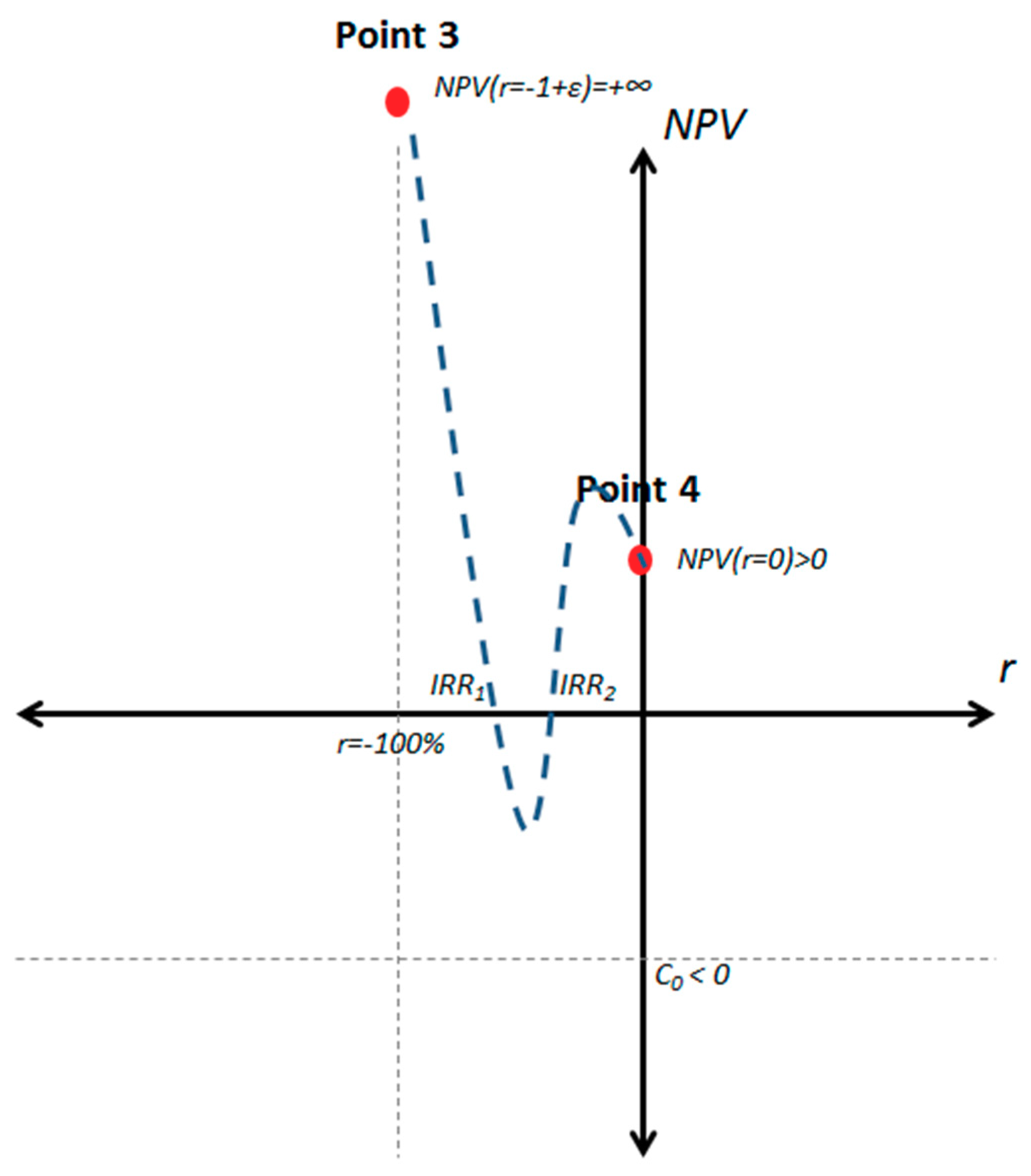
POINT 3: Right of the asymptote:

$$\underset{r\to -1+\epsilon }{\lim }NPV\left(r\right)=c_0+\frac{c_1}{+\epsilon }+\frac{c_2}{{\left(+\epsilon \right)}^2}+\dots +\frac{c_n}{{\left(+\epsilon \right)}^n}.$$

(10)

At this point the function will approach +∞ or −∞, depending on the sign of c_n; that will be negative if the number of sign changes on the cash flow stream is an even number, and will be positive otherwise.

POINT 4: The point at which the function cuts the NPV axis, that is, $NPV\left(0\right)={{\displaystyle \sum }}_{i=0}^n{c}_i$. This might be positive or negative.

POINT 5: As the value of r approaches +∞:

$$\underset{r\to +\infty }{\lim }NPV\left(r\right)=c_0+\frac{c_1}{+\infty }+\frac{c_2}{{\left(+\infty \right)}^2}+\dots +\frac{c_n}{{\left(+\infty \right)}^n}=c_0.$$

(11)

As stated before, c₀ < 0.

Since we are concerned about the number of real IRRs in the interval (−1, +∞) (real positive IRRs are located in the interval (0, +∞) - nevertheless, the Descartes rule of signs applies to the interval (−1, +∞)) the analysis focuses on points 3, 4 and 5. The value of point 3 depends on the number of sign changes on the cash flow stream. The value of point 4 may be positive or negative. The value of point 5 will always be (+∞, c₀ < 0). Thus, there are six potential situations, as shown in

Table 2. Potential value of key points on the net present value (NPV)(r) function on the interval [0, +∞). Source: Self-elaboration.

Value of NPV(0)	Odd Number of Sign Changes in the Cash Flow Stream	Even Number of Sign Changes in the Cash Flow Stream
NPV(0) > 0	POINT 3: (−1 + ε, +∞) POINT 4: (0, NPV(0) > 0)	POINT 3: (−1 + ε, −∞) POINT 4: (0, NPV(0) > 0)
NPV(0) = 0	POINT 3: (−1 + ε, +∞) POINT 4: (0, 0)	POINT 3: (−1 + ε, −∞) POINT 4: (0, 0)
NPV(0) < 0	POINT 3: (−1 + ε, +∞) POINT 4: (0, NPV(0) < 0)	POINT 3: (−1 + ε, −∞) POINT 4: (0, NPV(0) < 0)

.

These results provide us with valuable information regarding the number of real IRRs that may exist in the intervals (−1, 0) and (0, +∞). As an example, let us examine for instance the scenario with an odd number of sign changes in the cash flow stream and NPV(r = 0) > 0.

Interval (−1, 0): Point 3 and point 4 are above the horizontal axis. This means that the number of times that the NPV(r) function crosses the horizontal axis must be either 0, or an even number of times, as shown in Figure 1.

Proposition 1.

If an investment project has an odd number of sign changes on its cash flow stream and NPV(r = 0) > 0 (or an even number of sign changes on its cash flow stream and NPV(r = 0) < 0), then there are either 0 or an even number of real IRRs in the interval (−1, 0). It follows that an investment project with an even number of sign changes on its cash flow stream and NPV(r = 0) > 0 (or an odd number of sign changes on its cash flow stream and NPV(r = 0) < 0), then there is an odd number of real IRRs in the interval (−1, 0) (at least one).

As an example, consider the cash flow stream described in Table 1. It has an even number of sign changes (two) and NPV(r = 0) is < 0 (it is −2). According to Proposition 1, this cash flow stream should have 0 or an even number of real IRRs in the interval (−1, 0), which is consistent with the fact that it has 0 real IRRs on that interval.

Interval (0, +∞): Taking a look at point 4 (which is above the horizontal axis) and at point 5 (which is below the horizontal axis) in Figure 2 it can be deduced that the NPV^® function must cross at least once this axis in the interval [0, +∞), so there must be at least one real positive IRR. There may be more than one real positive IRR, but since point 5 is below the horizontal axis the total number of real positive IRRs must be an odd number, as shown in Figure 2.

Proposition 2.

If an investment project has NPV(r = 0) > 0, then there is an odd number of real positive IRRs in the interval (0, +∞) (at least one). It follows that if an investment project has NPV(r = 0) < 0, then there is either 0 or an even number of real positive IRRs in the interval (0, +∞).

Applying Proposition 2 to the cash flow stream described in Table 1, that has NPV(r = 0) < 0, it follows that the investment should have either 0 or an even number of real positive IRRs in the interval (0, +∞). This is consistent with the fact that this investment has two real IRRs bigger than 0.

If NPV(r = 0) = 0, the number of real positive IRRs will depend on what happens immediately to the right of point 4. That is:

$$\underset{r\to 0+\epsilon }{\lim }NPV\left(r\right)=c_0+\frac{c_1}{1+\epsilon }+\frac{c_2}{{\left(1+\epsilon \right)}^2}+\dots +\frac{c_n}{{\left(1+\epsilon \right)}^n}.$$

(12)

If this value is greater than 0, then there will be an odd number of real positive IRRs. If this value is smaller than 0, then there will be 0 or an even number of real positive IRRs. Since it may be complicated to determine whether the limit expressed in Equation (12) is greater or smaller than 0, the following proposition is provided.

Proposition 3.

If an investment project has NPV(r = 0) = 0, has an even number of sign variations and does not present a maximum in r = 0 (that is, NPV’(r = 0) ≠ 0), then the number of real positive IRRs is an odd number (at least one). It follows that if an investment project has NPV(r = 0) = 0, has an odd number of sign variations and does not present a minimum in r = 0 (that is, NPV’(r = 0) ≠ 0), then the number of real positive IRRs is either 0 or an even number.

These three propositions are summarized in

Table 3. Number of real positive IRRs depending on the value of NPV(0). Source: Self-elaboration.

	Number of Real Positive IRRs
NPV(0) > 0	Odd number (at least one)
NPV(0) < 0	0 or an even number
NPV(0) = 0	If even number of sign variations and NPV’(0) ≠ 0	Odd number (at least one)
	If even number of sign variations and NPV’(0) ≠ 0	0 or an even number

.

4.3. Combining the Descartes Rule of Signs with the NPV(r) Function Characteristics

Interesting as these results may be, they do not help much in narrowing down the number of real positive IRRs. Nevertheless, when we combine the Descartes rule of signs, based on the number of sign variations in the cash flow stream, with the insights provided in Table 3 (based mainly on the value of NPV(r = 0)) it is possible to narrow down the number of real positive IRRs. Consider for instance a cash flow stream with NPV(r = 0) > 0 and try to determine the number of real positive IRRs. The results of this exercise are included as Appendix A, that have been summarized in

Table 4. Number of real positive IRRs depending on the value of NPV(r = 0) and the sign variations in the cash flow stream. Source: Self-elaboration.

NPV(r = 0)	Sign Variations in the Cash Flow Stream	Real IRRs (0, +∞)
> 0	1	1
> 0	2	1
> 0	3	3, 1
> 0	4	3, 1
> 0	5	5, 3, 1
> 0	6	5, 3, 1
> 0	7	7, 5, 3, 1
> 0	…	…

in order to arrive at certain conclusions.

Proposition 4.

If an investment project has NPV(r = 0) > 0, then it has an odd number of real positive IRRs that is equal or smaller than the number of sign variations on its cash flow stream. If an investment project has NPV(r = 0) < 0, then it has either 0 or an even number of real positive IRRs that is equal or smaller than the number of sign variations on its cash flow stream.

Looking at the cash flow presented in Table 1, it has NPV(r = 0) < 0 and two sign changes. According to Proposition 4, it should have either 0 or two real positive IRRs consistent with the two real positive IRRs it already has.

These results allow to determine sufficient conditions for a single positive real root and are in agreement with the conclusions reached by other authors and presented in the state-of-the-art, such as the conclusions reached by Ben-Horin and Kroll [25] for cash flow streams with two sign variations. Furthermore, it can be sometimes used when Norstrom’s criterion is inconclusive. Consider for instance the example in

Table 5. Cash flow stream that is inconclusive for Norstrom’s criterion. Source: Self-elaboration.

Year	Cash Flow	Cumulative Cash Flow
0	+2000	+2000
1	−500	+1500
2	−8100	−6600
3	+6800	+200

.

The cumulative cash flow has two sign changes, making Norstrom’s criterion inconclusive. Using Proposition 4 and considering that the cash flow has two sign changes and NPV(r = 0) > 0, we can conclude that the cash flow has an odd number of real positive roots smaller than 2, so it can only have one real positive root.

5. Results

The Descartes rule of signs was meant for polynomial equations, and the NPV is not a polynomial. Nevertheless, the Descartes rule of signs can be reinterpreted in order to establish a sufficient condition for a single positive real root.

The NPV function has, as previously stated, the following structure:

$$NPV\left(r\right)=c_0+\frac{c_1}{1+r}+\frac{c_2}{{\left(1+r\right)}^2}+\frac{c_3}{{\left(1+r\right)}^3}+\dots +\frac{c_n}{{\left(1+r\right)}^n},$$

(13)

This means that, as r reaches higher positive values, the value of 1 + r increases and the terms that are divided by 1 + r decrease in absolute value. But not all terms divided by 1 + r decrease at the same pace: The higher the power of 1 + r the faster the term will decrease; for instance, $\frac{1}{{\left(1+r\right)}^2}$ decreases faster than $\frac{1}{1+r}$. Since we know that in the end the c₀ coefficient will become dominant, which is negative, there will be only one real positive root if the NPV(r) function changes one time in value on the (0, +∞) interval, from positive to negative.

Let us assume that we have an NPV(r) function with only two terms, the first one negative and the second one positive.

$$NPV\left(r\right)=-c_0+\frac{c_1}{1+r},$$

(14)

In order for this function to have a real positive root, it is absolutely necessary that the following condition is met:

$$\left|c_0\right|<\left|c_1\right|,$$

(15)

In this way, NPV(0) is a positive value. As the value of r increases, the first term of the NPV function remains unchanged, but the absolute value of the second term starts to decrease. At one point, NPV(r) will be equal to zero (a real positive root), and then it will continue to reach increasingly negative values.

Repeating the exercise with an NPV function that has three terms and two sign variations, the same logic described previously can be applied.

$$NPV\left(r\right)=-c_0+\frac{c_1}{1+r}-\frac{c_2}{{\left(1+r\right)}^2}.$$

(16)

As r increases, the second and the third term of the function will decrease. The third term however decreases faster than the second term. If we want to have a single real positive root for the NPV function, then the only solution is for NPV(r) to initially have a positive value and just make one transition into a negative value. This will require that the second term starts dominating over the first and third terms and then, as r increases, at one point the first and third term dominates over the second one. The necessary condition could then be expressed as follows:

$$\left|c_0+c_2\right|<\left|c_1\right|,$$

(17)

An NPV function with three sign variations can also be analyzed.

$$NPV\left(r\right)=-c_0+\frac{c_1}{1+r}-\frac{c_2}{{\left(1+r\right)}^2}+\frac{c_3}{{\left(1+r\right)}^3},$$

(18)

This function may have one real positive root only if the value of the function NPV changes from positive to negative only once. For this to happen it is enough that the following condition is met:

$$\left|c_0+c_2\right|<\left|c_1\right|,$$

(19)

That is to say, it is enough for the positive terms between the first and second change of sign to be so big that they cancel out the negative terms, until eventually a large enough value of r will make the initial negative values predominant.

Proposition 5.

If the terms of an investment project NPV function are ordered by descending variable exponent, then there is only one real positive root if the sum of the positive coefficients between the first and second changes of sign (that all of them must be positive) is bigger in absolute value than the sum of all the negative coefficients.

Let us consider the cash flow stream presented in Table 1. The sum of the positive coefficients between the first and second changes of the sign (which add up to 7.5) is not bigger in absolute value than the sum of all the negative coefficients (which add up to −8.5). We cannot be certain that there is only one real positive IRR; in fact, there are two.

Consider now the cash flow stream shown in

Table 6. Example of a cash flow stream that complies with Proposition 5. Source: Self-elaboration.

Period	0	1	2	3	4	5	6	7	8
Coefficient	c0	c1	c2	c3	c4	c5	c6	c7	c8
Cash flow	−30	15	30	−5	8	−3	10	−5	15

.

The sum of the positive coefficients between the first and second changes of sign (c₁ + c₂) is 45, bigger than the absolute value of the sum of all the negative coefficients (c₀ + c₃ + c₅ + c₇) that add up to 43. It can be concluded that this cash flow has only one real positive IRR, which happens to be 38.6%.

Consider now that we have an NPV(r) function with four changes in sign:

$$NPV\left(r\right)=-c_0+\frac{c_1}{1+r}-\frac{c_2}{{\left(1+r\right)}^2}+\frac{c_3}{{\left(1+r\right)}^3}-\frac{c_4}{{\left(1+r\right)}^4},$$

(20)

Beyond what was established in Proposition 5, another way for this investment to have a single real positive root would be to meet the following condition:

$$\begin{gathered} \left|c_0+c_2\right|<\left|c_1\right|, \\ \left|c_4\right|<\left|c_3\right|, \end{gathered}$$

(21)

If these two conditions are met, then the NPV(0) is positive and will remain so until the r is large enough for c₀ to become the dominant coefficient.

Proposition 6.

If the terms of an investment project NPV function are ordered by descending variable exponent, then there is only one real positive root if the sum of the positive coefficients between sign changes are bigger than the absolute value of the sum of the negative coefficients that follow before the next change of sign, and NPV(0) has a positive value.

Consider the cash flow in

Table 7. Example of a cash flow stream that satisfies Proposition 6. Source: Self-elaboration.

Period	0	1	2	3	4	5	6	7	8
Coefficient	c0	c1	c2	c3	c4	c5	c6	c7	c8
Cash flow	−30	−10	15	−2	20	−16	35	−5	−3

.

The sum of the positive coefficients between sign changes are systematically bigger than the absolute value of the sum of the negative coefficients that follow before the next change of sign:

• c₂ = 15 > |c₃| = 2
• c₄ = 20 > |c₅| = 16
• c₆ = 35 > |c₇ + c₈| = 8

Furthermore, this cash flow has a positive NPV(0) = 4. It can be concluded that there is only one real positive IRR (4.6%).

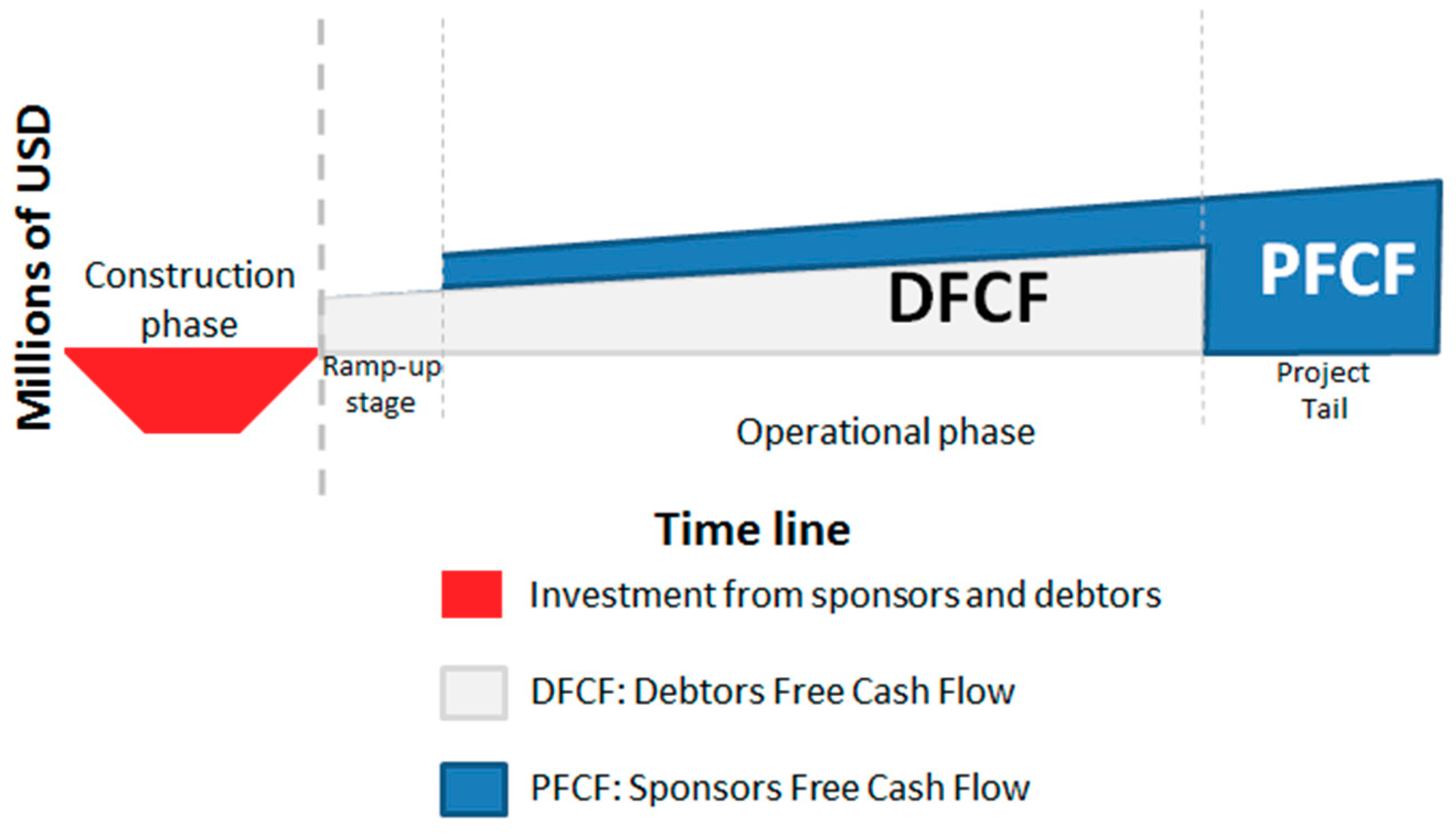
Also, the following combination would achieve the same result; very relevant for instance for Public Private Partnership projects, in which most of the shareholder dividends are concentrated at the end of the project:

$$\left|c_0+c_2+c_4\right|<\left|c_3\right|,$$

(22)

Proposition 7.

If the terms of an investment project NPV function are ordered by a descending variable exponent, then there is only one real positive root if the two following conditions are met simultaneously:

• The sum of the last positive coefficients between sign changes is bigger than the absolute value of the sum of all the negative coefficients, and
• The sum of the other positive coefficients between sign changes is smaller than the absolute value of the sum of the negative coefficients that precede them before the previous change of sign.

Consider the cash flow in

Table 8. Example of a cash flow stream that satisfies Proposition 7. Source: Self-elaboration.

Period	0	1	2	3	4	5	6	7	8
Coefficient	c0	c1	c2	c3	c4	c5	c6	c7	c8
Cash flow	−20	−10	10	7	−15	10	−10	20	40

.

The sum of the last positive coefficients between sign changes is c₇ + c₈ = 60. This is bigger than the absolute value of the sum of all the negative coefficients (|c₀ + c₁ + c₄ + c₆| = 55). Also, the sum of the other positive coefficients between sign changes is systematically smaller than the absolute value of the sum of the negative coefficients that precede them before the previous change of sign:

• c₂ + c₃ = 17 < |c₀ + c₁| = 30
• c₅ = 10 < |c₄| = 15

It can be concluded that there is only one real positive IRR (18.0%).

These propositions complement the work discussed by other authors and presented in the state-of-the-art, and in particular the work performed by Carey (2012).

6. Application to Cash Flows from PPP Projects

According to Ben-Horin and Kroll [25] the problem of multiple IRRs is very unlikely to occur in cash flow structures that have an economic appeal to practitioners. Three or more sign variations occur when there is at least one intermediate negative future cash flow, that typically represents (when the cash flow is unlevered) an option rather than an obligation to reinvest. Under this assumption, the positive expected value of the option should substitute the future reinvestment, and there are no multiple IRRs.

There are situations, however, in which the above statement may not apply. One situation for instance is PPPs involving large-scale infrastructure projects over a long period of time (several decades). It is normal in these projects to have important reinvestments at several times; for example, in order to renew the rolling stock of a subway line. In these arrangements, however, the private investor of the project does not have the option to exit the project at the time of the reinvestment if the expected value of the future cash flows that the investor expects to receive until the end of the contract is not greater than the reinvestment itself. In these projects the private investor is usually under the obligation to create a reserve fund and other provisions in order to make sure that these re-investment obligations are met. In practice this means that the cash flow stream would not present sign changes, there would be just lower dividends along the way. Thus, the cash flow of a PPP project is almost certain to have a negative value during the preparation and construction phase, and then a positive value during the operational phase (see for instance the examples presented by Esty [32] and Weber et al. [33]. Under a simplified scheme, the after-tax shareholder cash flow of a PPP project usually adopts the configuration shown in Figure 3 [34]:

Therefore if the cash flow stream of a PPP project usually has only one sign variation and NPV(r = 0) greater than zero, according to Proposition 4 it can be concluded that it will have only one real positive IRR.

7. Conclusions

This paper demonstrates that when the sum of the cash flows of an investment project in nominal terms is greater than 0, then it has an odd number of real positive IRRs that is equal or smaller than the number of sign variations on its cash flow stream.

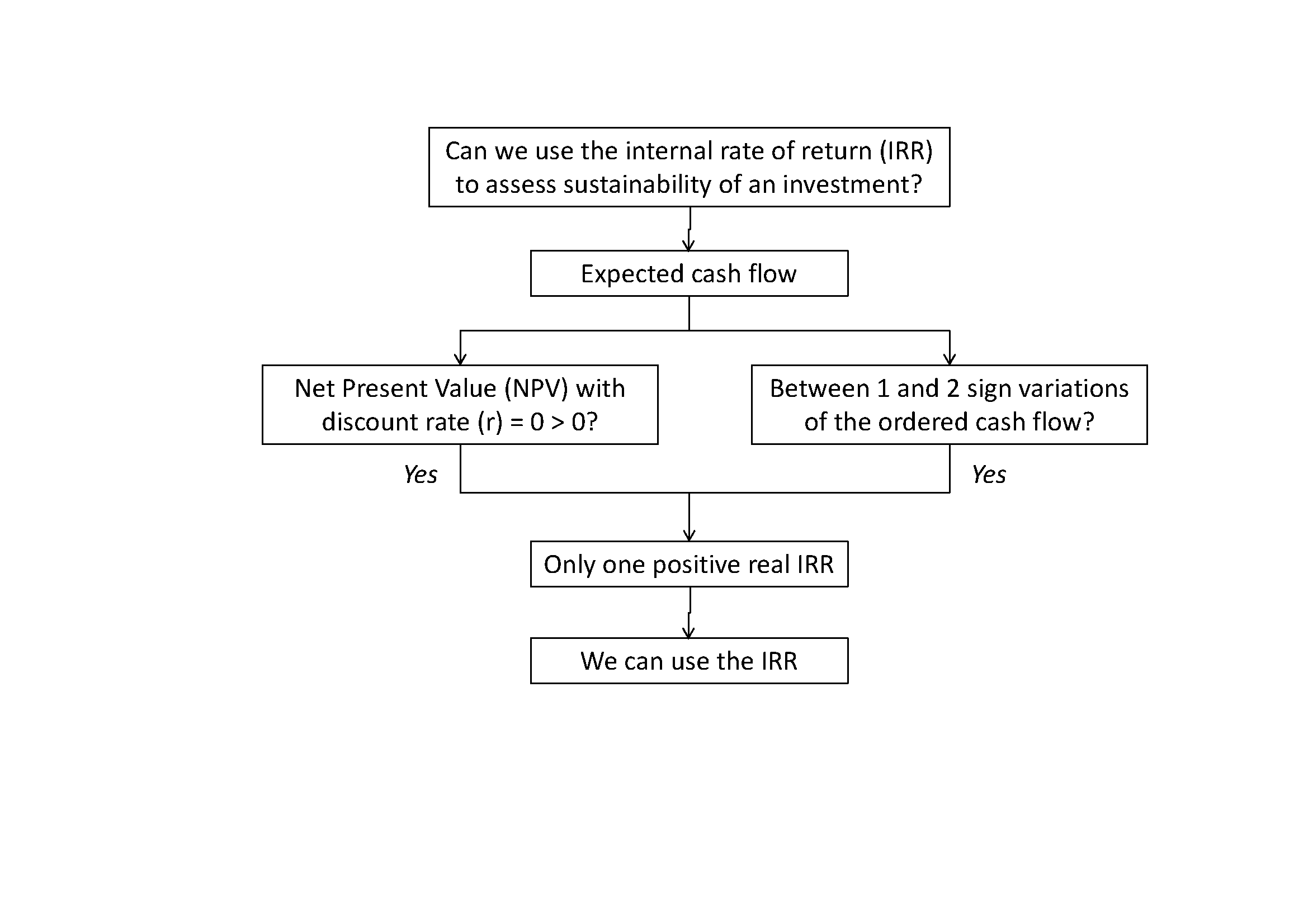
This paper also determines that the usual PPP investment project has a single sign variation on its cash flow stream, from negative to positive. This sign variation signals the end of the construction stage and the beginning of the operation and maintenance phase.

Under these conditions, it can be concluded that PPPs have a single real positive IRR. The general use of the IRR as a criterion to assess the sustainability of PPP investments is thus validated. There may be however PPP projects with singular cash flow structures, with more than one sign variation—the IRR criterion should be used with caution in these circumstances.

A further analysis of the NPV function, its coefficients and its sign variations allow to obtaining further propositions concerning the potential number of real positive IRRs that a cash flow may present. Propositions 5, 6 and 7 presented in this article are the results of such analysis.

This study complements current academic PPP literature within the “Policy of PPPs” category, and in particular within the “Risk management and financial evaluation” category, as described by Roechrich et al. [4]. Within the financial academic literature, this paper provides a novel proposition that can be used to determine if a cash flow has a single real positive root when other existing propositions fail.

Future research could further explore the value creation in PPP projects from the perspective of the private sector, as well as providing a convincing reason to explain why multiple real IRR for a particular cash flow is of practical use.