Article

Model and Simulation of a Floating Hybrid Wind and Current Turbines Integrated Generator System, Part I: Kinematics and Dynamics

Instituto de Automática e Informática Industrial ai2, Universitat Politècnica de València, Camino de Vera s/n, 46022 Valencia, Spain
*
Author to whom correspondence should be addressed.
J. Mar. Sci. Eng. 2023, 11(1), 126; https://doi.org/10.3390/jmse11010126
Submission received: 3 October 2022 / Revised: 16 December 2022 / Accepted: 28 December 2022 / Published: 6 January 2023
(This article belongs to the Section Ocean Engineering)

Abstract

:
This initial publication is part of a series of publications that will appear soon, which pursue a final objective for the proposal of a fully integrated and controlled hybrid system composed of a floating wind turbine—type “OC3-Hywind”—and two marine current turbines with the aim of increasing the energy generated by the floating installation and, at the same time, use the set of turbines as actuators as part of an integral cooperative control system of the floating hybrid system to ensure the structural stability of the floating hybrid generator system (FHGS) in harsh weather conditions, which is a key issue in this type of floating systems. A specially designed tool to design, analyze, and control this type of FHGSs was developed using Matlab®. In this tool, named Floating Hybrid Generator Systems Simulator (FHYGSYS), several tests were carried out on the structural stability of the system considering the interactive phase of the acting forces. Working in a programming environment like Matlab® allows design freedom and the possibility of evaluating the system with different geometries, aerodynamic airfoils, and external meteorological conditions, and also including or eliminating certain elements, etc. This versatility will be helpful in future studies aimed at evaluating this system and maximizing the production of energy.

1. Introduction

Wind energy extraction techniques have evolved from the first wind turbines installed on land, allowing the increase in their size with the objective of generating more electricity. At the same time, the idea of using the potential energy from the sea to produce electricity is being consolidated in recent years. Additionally, different energy generation systems are currently under development to achieve the capacity of extracting energy from waves, tides, or marine currents [1,2].
Floating wind turbines (FWT) [3,4] are the alternative to offshore wind power generation for depths greater than 60 m. Operating at a distance from coasts involves using more important wind resources and reducing the visual and noise impact. Nevertheless, the floating nature of these devices involves stability requirements to account for the control system further than the power production.
The first prototype [5], Blue H, was installed in 2008 in a water depth of 113 m. Since then, researchers and firms have commissioned other prototypes.
Windfloat® is a patented FWT developed by Principle Power Inc [6]. The Windplus consortium used this wind turbine (WT) to design the first floating wind farm in offshore Portugal [7]. The first turbine was installed in 2010, and, in July 2020, the floating wind farm was fully operational. WindFloat Atlantic is grid-connected to Portugal, generating up to 25 MW.
RWE Global is also working on FWT prototypes [8]. DemoSATH is a 2 MW turbine over a concrete structure [9]. The prototype has a single point of mooring that provides self-alignment to the current and wave direction. This project is installed on the north coast of Spain. TetraSpar is a 3.6 MW turbine over a tubular steel structure [10]. The prototype test site is located in Denmark, 10 km offshore with a depth of 200 m. Aqua Ventus is an 11 MW WT over a concrete semi-submersible structure [11]. This project is expected to be operative in 2024 in New England (USA).
A disrupting FWT system is being developed by X1wind [12]. This firm developed PivotBuoy® [13], a system capable of self-orientating the floating turbine to maximize the generated power, thus reducing the weights, making FWT more competitive.
Real prototypes and scientific research [14,15] show that the control of FWTs faces challenges that cannot be overcome with conventional power control techniques. High structural loads or platform movement due to wave currents and tidal forces impose stability restrictions not considered in traditional WT control. This vital requirement has pointed to the need for advanced predictive control and condition monitoring techniques to preserve structural stability and integrity, as opposed to conventional power control techniques.
In a conventional wind turbine with structural support to the ground, the angular displacement of the tower is relatively small, even under challenging wind conditions. The axial force of the wind mainly causes bending moments in the tower. Under these conditions, the weight of the nacelle acts by compressing the tower, not bending it.
The dynamics of large horizontal axis wind turbines—with structural support to the ground—can be modeled using a five-degree-of-freedom model. The dominant modes [16] include:
  • out-of-plane deflection of the blade flap rotor;
  • in-plane deflection of the blade edge;
  • fore-and-aft tower motions;
  • powertrain roll and twist.
As suggested in Figure 1, the dynamics of the deformations associated with these degrees of freedom tend to be coupled.
For example, the tower fore–aft motion is strongly coupled to the blade flap motion, and the tower roll motion is strongly coupled to the blade edge and power train torsion.
In this context, large modern WTs allow the application of control techniques that make possible an independent adjustment of the pitch angles of each blade [17]. Individual pitch control extends the conventional objectives of pitch control to reducing fatigue loads, particularly by active damping tower oscillations.
In the case of complex floating systems with six degrees of freedom, the system behaves as a mass–spring–damper system affected by changing forces resulting from wind flows and hydrodynamic forces due to waves and marine currents. Under certain conditions of higher-than-normal wind speed, conventional pitch control techniques introduce negative damping in the movement of the floating tower. That causes an excitation of the natural frequency and may cause the floating structure to resonate by applying decreases in the wind opposition when varying the pitch angle of the blades to regulate the active power generated. This phenomenon was observed in tests carried out at the Ocean Basin Laboratory at Marintek in Trondheim [18].
In an FWT, the support platform moves freely, and the tower can experience angular displacements of several degrees. In this case, the weight of the nacelle is directly related to the bending of the tower. Of note in this phenomenon are the effects of its amplitude and frequency. In terms of frequency, due to constantly varying wind and wave loads, significant fatigue stresses occur in the structure.
These considerations lead to the subjection of special operating conditions worthy of a detailed analysis, which can only be performed with the help of simulation software tools. Specifically, the simulation tool FAST [19] is to be highlighted for this purpose.
Additionally, to perform such an analysis, it is necessary to have a coupled dynamic behavior model of the floating support base and the tower/nacelle. This model will help us to define which variables should be monitored in the context of a condition monitoring system of the FWT structural system.
Attention must be paid to the interactions between the mechanical effects due to inertia loads (rotor, nacelle, and tower) and the electrical effects (generator, control, and protection systems).
The controller’s goal should be to minimize turbine and platform motion while limiting mechanical wear on the generator and transmission. In this sense, some simulation tools, such as FAST [20], have system linearization tools that can be used to design controllers based on the linear-quadratic gain theory. Another option is the design of controllers based on the Lyapunov theory for the minimization of energy functions. The FAST simulation tool was specifically developed to carry out pre-study tests on the overloads that can occur, among others, on the blades and tower of the floating wind turbines. It allows the testing of different control strategies, such as Gain Scheduling PID, LQR with Collective Blade Pitch, and LQR with Individual Blade Pitch or H∞.
Studies were initially conducted with individual target controllers for rotor speed regulation using collective blade pitch [21] for different FWT systems [22]. In the last ten years, individual pitch control has been the main trend in this area [23]. In [24], an individual pitch control scheme was developed to deal with blade and pitch actuator faults in FWTs. It is shown that, with these faults, conventional pitch control techniques fail. Modern techniques [25] (such as sliding control) have also been applied to pitch control in an FWT, with promising results. The proposed controllers can accomplish better power regulation, reducing the platform pitch motion and the blade load.
From the point of view of control engineering, hybrid FWT and marine current turbines (MCT) foundations are promising generators that can achieve more excellent stability than FWT. These foundations are a hot topic in the research and study of control algorithms and marine power generation. A series of objectives is raised that aim to develop advanced control, monitoring, and diagnostic algorithms for the maximum use of marine generation systems to increase the performance and structural stability of the system and ensure its economic viability.
The traditional objective of control systems applied to hybrid generation systems has been to maximize the energy generated. In the case of generation systems resting on a floating offshore platform, other requirements, such as structural stability, may be equally or more important. Due to the difficulty of access, costly maintenance, and expensive commissioning involved in having generators offshore, ensuring the physical integrity of the generator is the priority.
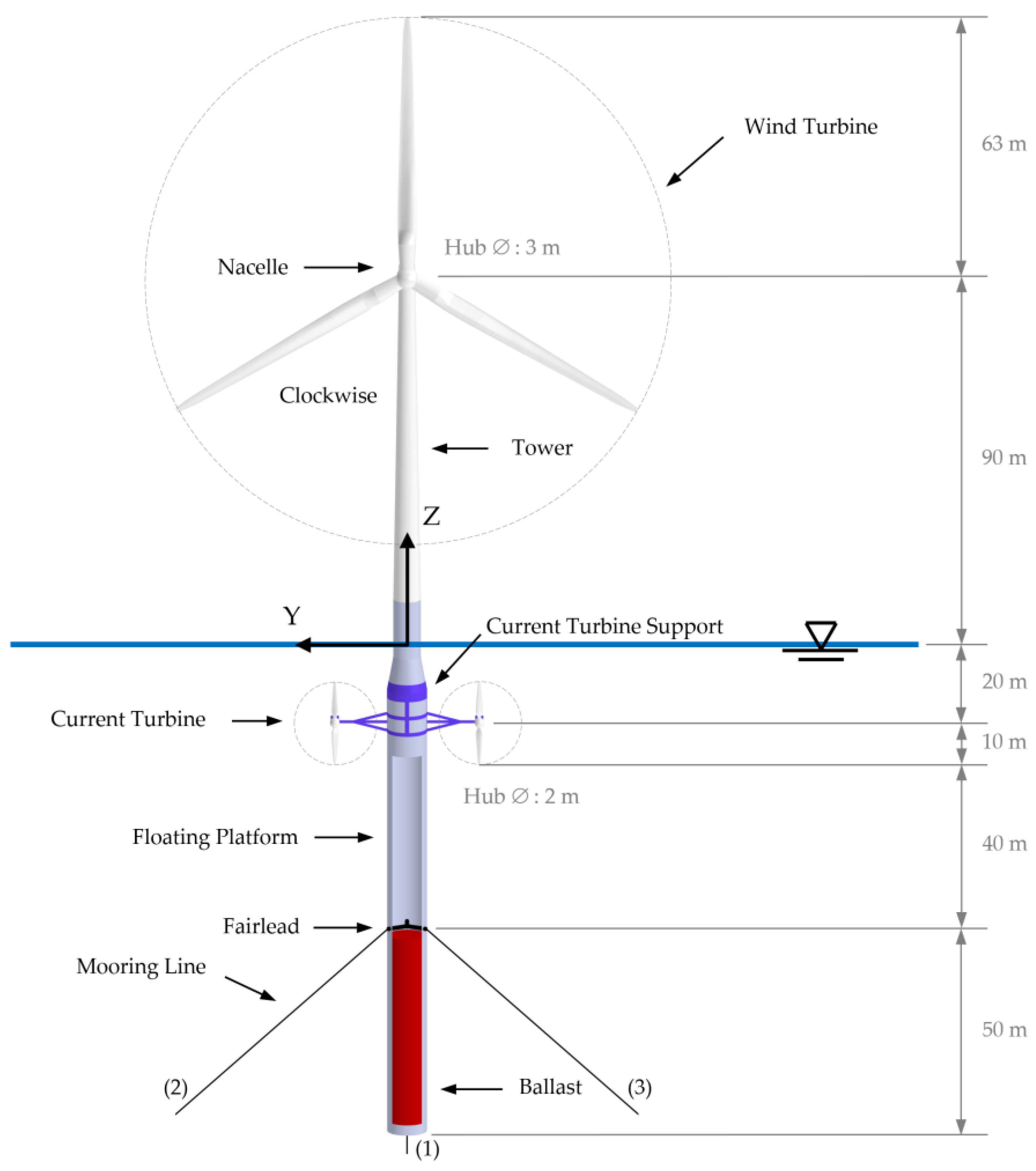
The hybridization offers an opportunity to address the problem of controlling the structural stability of the floating system. Stability enhancement has been considered a major challenge since the early days of floating wind turbine design. With this objective, in this work, a specific solution is exposed, consisting of a floating hybrid system composed of a wind generation subsystem and a generation subsystem with two marine current turbines. This proposal allows the development of an integrated control system which simultaneously deals with the structural stability of the system and the optimization of the generation capacity.
A hybrid system capable of taking advantage of both wind energy and marine currents to produce electricity with the aim of maximizing the performance of a structure installed in the sea was designed in [26,27,28,29,30]. In [26], the first version of this type of hybrid system called HYWIKIM was presented. In [27], the first behavioral hypotheses of HYWIKIM were exposed. In [28], a real HYWIKIM prototype was presented, which was tested at the Real Club Náutico de Valencia. In [29], the results of the tests carried out with HYWIKIM were extended and presented. In [
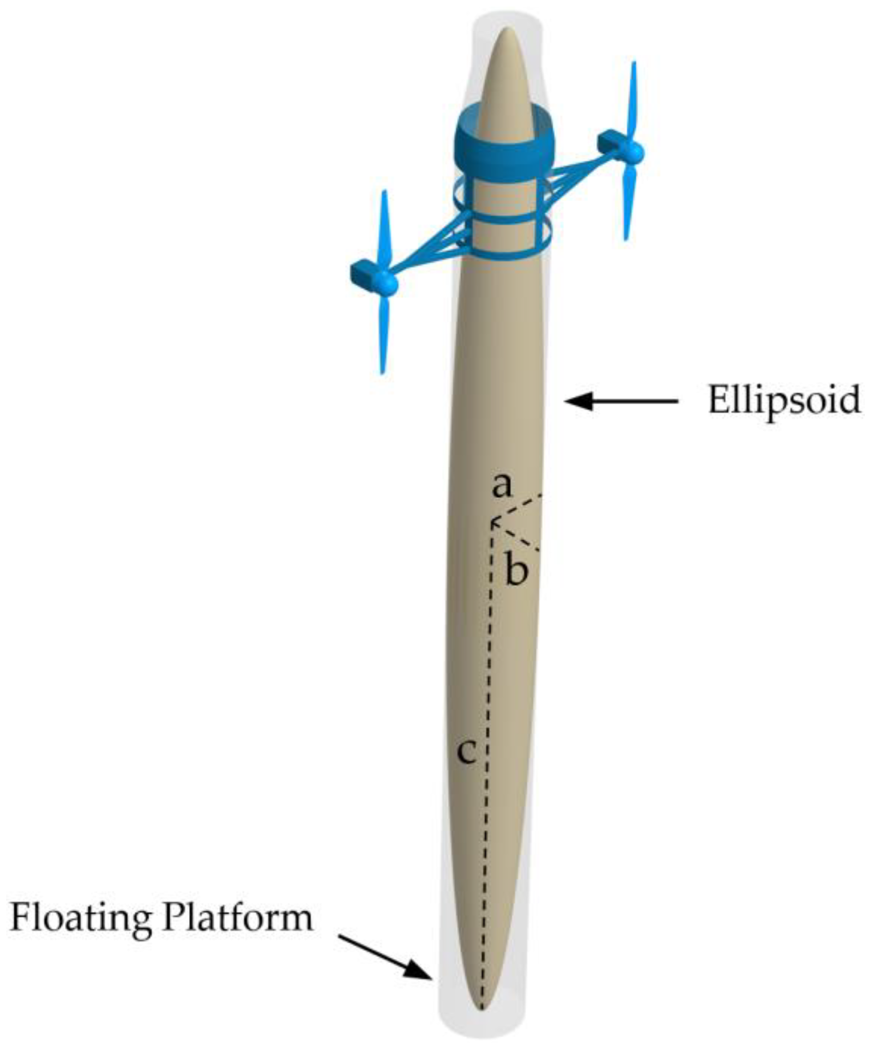
30], the first version of the mathematical model that allows the simulation of the behavior of this hybrid system concept was presented, using an “OC3-Hywind”-type floating wind turbine described in [31], to which two marine current turbines were coupled, as those described in [32].
The novelty of this proposal is that it introduces the concept of cooperative, integrated control of the two generation subsystems involved to counteract tendencies towards instability, which, if not avoided, reduce the useful life of the hybrid system. This issue is highlighted as especially important in [33]. This is an inherent problem with hybrid floating systems where, under certain circumstances, the applied pitch control can cause the floating system to resonate.
In order to effectively use tidal turbines together with wind turbines, the wind and current resources must coexist. In some cases, one—or both—of the natural resources can threaten the floating system’s stability. There are many places worldwide—generally in the straits—where wind resources [34] coexist with tidal currents capable of activating tidal turbines: wind speed above 10 m/s and tidal currents above 2 m/s. Examples of these kinds of locations (Table 1) are the Banks Strait in Australia [35], the Strait of Gibraltar in Spain [36], the Straits in Florida in the United States [37], the Strait of Malacca in Malaysia [38], the Dover Strait in England [39], the Euripus Straits in Greece [40], the Strait of Messina in Italy [41], the Cook Strait in New Zealand [42], the Alas Strait in Indonesia [43], The Bosporus Strait in Turkey [44], the tidal strait near Roosevelt Island in United States [45], or the Ushant Island [46,47]. The current speed depth ranges from 25 to 40 m. Therefore, turbines must be placed at the correct depth in each case to take advantage of these currents. In the case of low-speed locations, a mechanical augmentation channel [27] can be used to achieve the proper speed.
Although the design of the floating hybrid system was made by placing the marine current turbines at a depth of 20 m, the simulator can be adapted to carry out simulations by placing the marine current turbines at different depths, depending on the characteristics of the simulation site.
Continuing with the work carried out in [26,27,28,29,30], the authors plan to publish a series of articles that broaden the research in this field. It is intended to expose, in an exhaustive way, the mathematical modeling of the floating hybrid system carried out, dividing the exhibition into two publications—this being the first of them. Using this model, the study of the behavior of the hybrid system will be addressed by applying different control strategies. The series of works will be closed with a final installment in which the hybrid system will be evaluated by changing the characteristics of the elements that compose it: length and number of blades of marine turbines, different aerodynamic profiles, different number of mooring lines, etc.
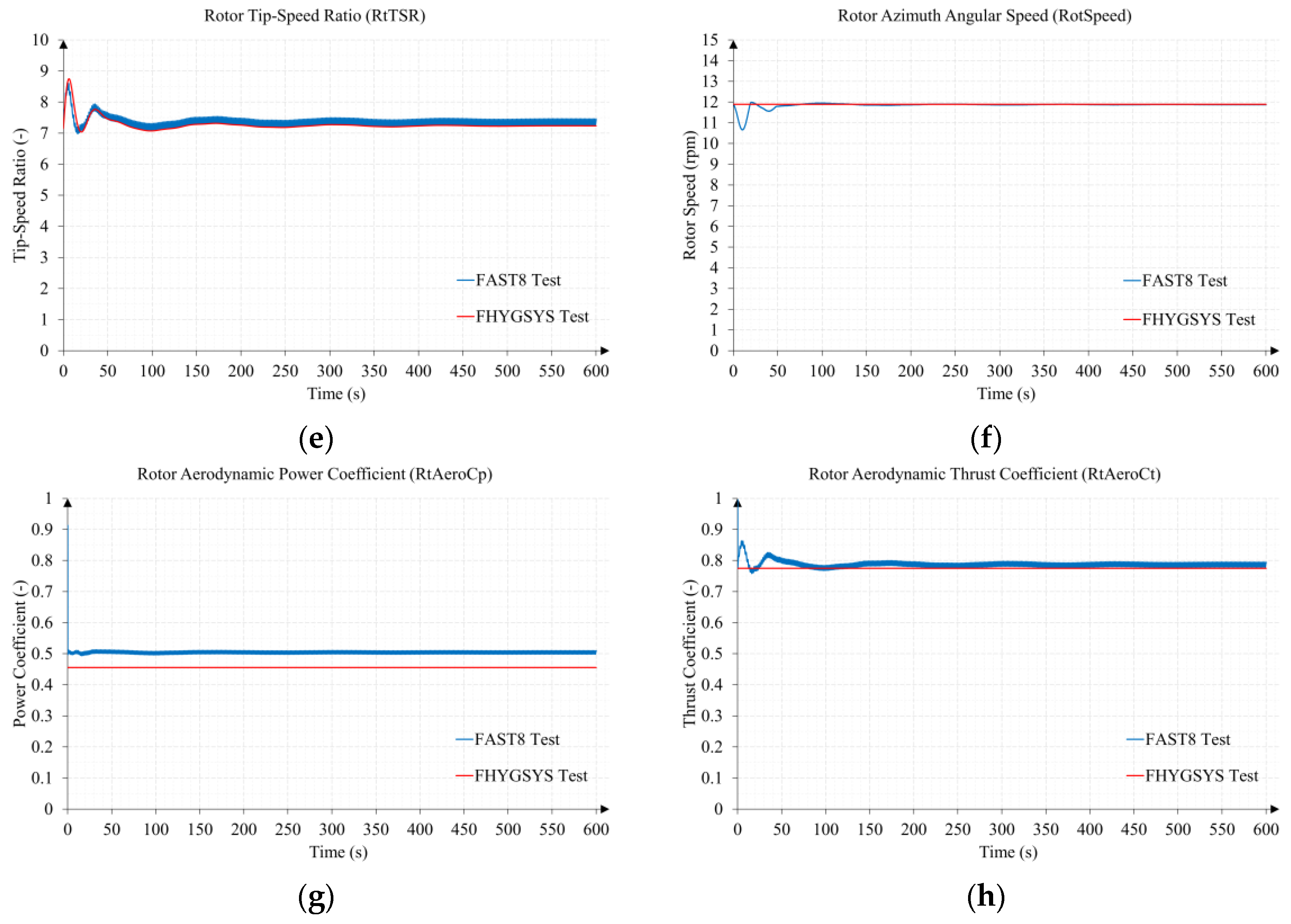
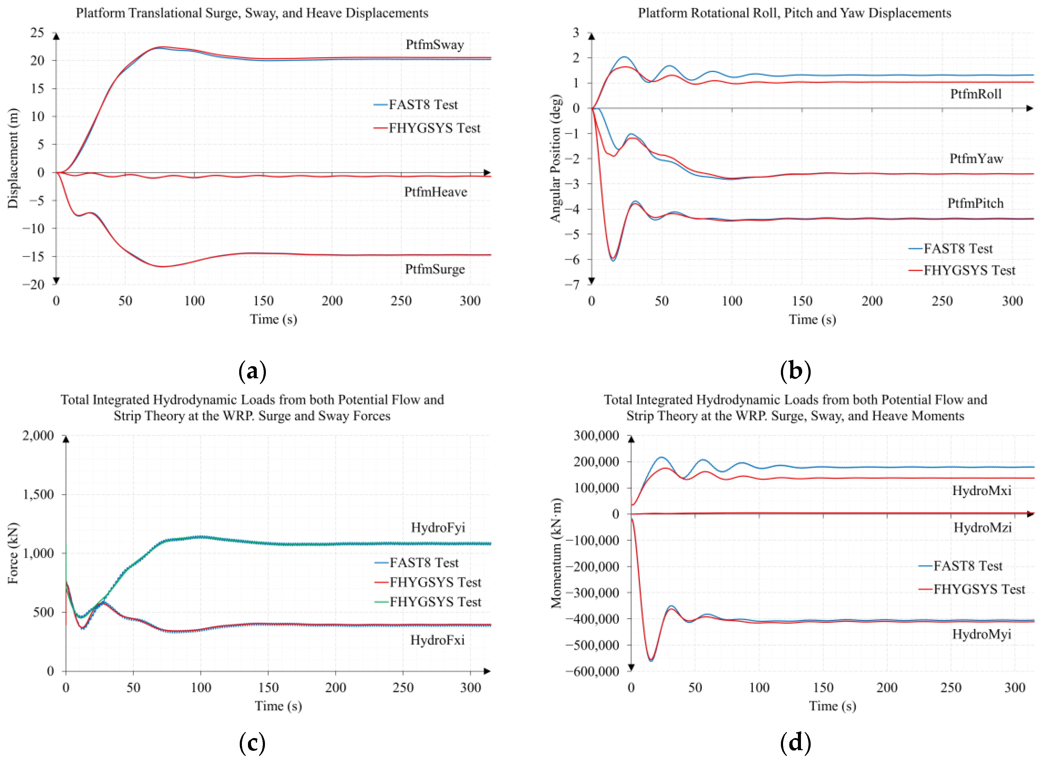
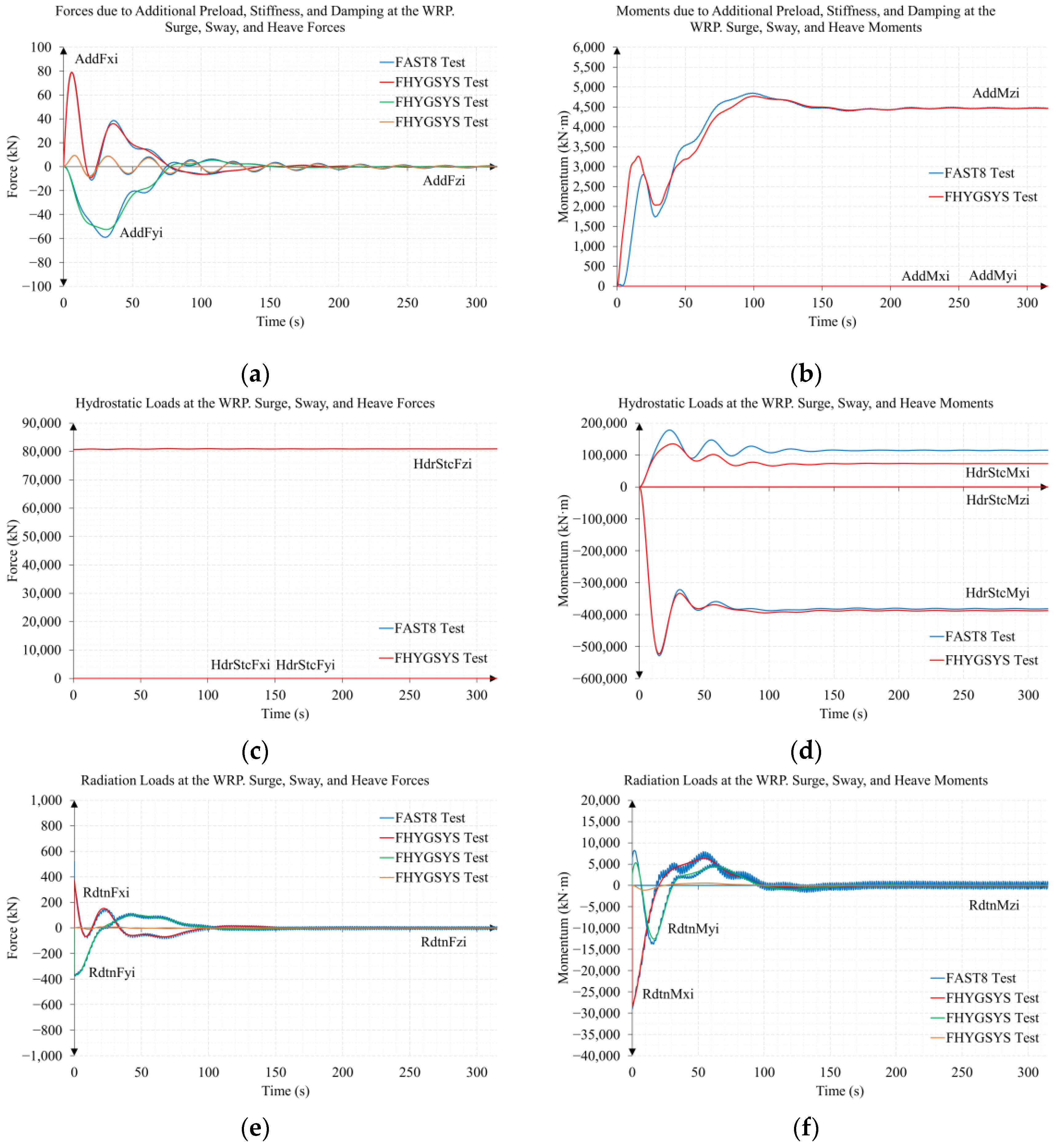
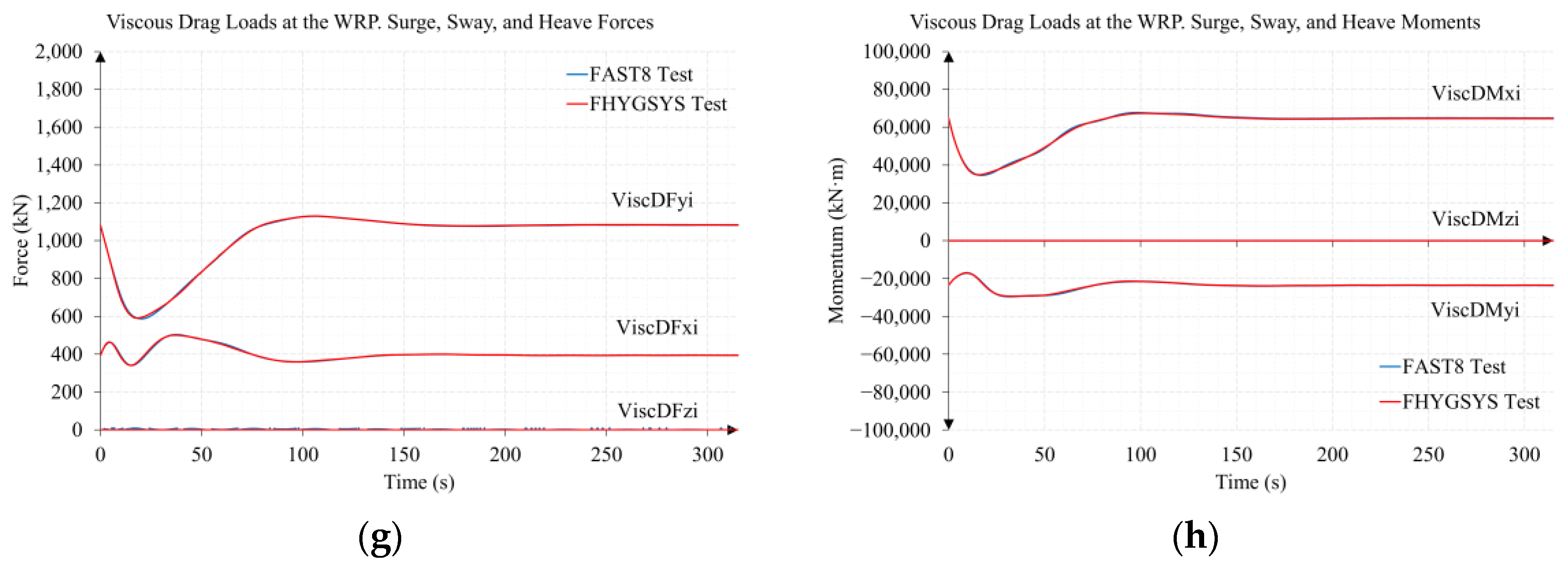
In this work, the first version of the FHYGSYS tool is introduced using the one-dimensional theory to compute the thrust of the turbines. This theory allows the obtainment of a good approximation to know which behavior the steady state response system will have. The operational capacity of the tool was validated by comparing the results with the certificated test of the OC3-Hywind calculated in FAST 8. This comparison is offered in Appendix E.
Why did we choose to develop our own tool like FHYGSYS? Mainly because, when the research line began, there was no simulation tool that would clearly allow the simulation of marine current turbines, offering the possibility of freely designing different control strategies. The main objective of the research is precisely that: to study the behavior of a hybrid floating system like the one described using different automatic control strategies.
On the other hand, this research has allowed the development of a deep understanding of the mechanics of this type of complex system. In addition, the developed modeling techniques can be applied not only to floating systems, but also to any mechanical system. This offers a relatively easy path for the macroscopic modeling of mechanical systems, for example, for modeling systems in automatic control engineering.
This paper is structured as follows: Section 2.1 and Section 2.2 introduce the initial assumptions for the development of the tool. Section 2.3 exposes the mathematical model, showing the methodology followed for both kinematic and dynamics calculations. Next, Section 2.4, describes the forces that were considered relevant for the development of the mathematical model, but leaving their exhaustive explanation to the second part of this publication. Section 3 explains the results obtained in the performed tests. Finally, Section 4 presents the discussion and future work for this line of research.

2. Materials and Methods

2.1. Floating System

There are different solutions to the problems involved in installing wind turbines in the sea—some of them are compared in [48]. The solution chosen in this work is the one used in phase IV in the “OC3” project [31,49]. There are multiple studies about this solution, and thus, it can be considered a standard that allows us to easily compare the results obtained. This configuration is called “OC3-Hywind” [31,49] and is composed of a 5MW wind turbine [50] mounted on a spar-buoy floating platform [31]. It has a mooring system consisting of three lines anchored to the seabed [31,51], which prevents the floating system from drifting.
Continuing with the work carried out in [26,27,28,29,30], a mathematical model of a hybrid system capable of taking advantage of both wind energy and marine currents to produce electricity is developed (Figure 2).
The hybrid system is equipped with two marine current turbines (Figure 3) based on the designs described in [32,52]. These turbines perform a double function:
  • the generation of electricity taking advantage of the kinetic energy transmitted by marine currents: in this situation, the system operates in a cooperative mode as a wind turbine and a double marine generator;
  • contribution to the stabilization of the floating structure in hard weather conditions: in this situation, the system works in an active stabilization mode using the set of existing turbines as a cooperative control for system stabilization.

2.2. Modeling Hypothesis

For the realization of the mathematical model of the system, several modeling hypotheses were considered.
The mathematical model does not consider the flexible behavior of the structural elements from the system. Therefore, the mechanical analysis is carried out considering a structure composed of a set of rigid solids that cannot deform. This permits the location of their position just by placing a point belonging to the system in the Euclidean space. In principle, this simplification does not represent a considerable error related to the movement of the floating platform [49] and implies that the internal behavior of the different bodies from the floating system is ignored.
The floating system is moored to the seabed through three flexible lines. Their characteristics are found in [31,51].
The geometric depiction of the model is conducted using orthogonal systems of Cartesian coordinates. Two coordinate systems were mainly considered: a fixed inertial one (X, Y, Z) and a mobile one (x, y, z) that move together with the rigid solids from the floating system. Unless otherwise indicated, when reference is made to specific coordinates in this work, they will always refer to the inertial coordinate system (X, Y, Z) [51]. In the initial position, the origin of the two-coordinate systems match, only separating when some external force acts on the floating structure.
To represent the position of the floating system, six degrees of freedom were used (Figure 4), with three translations—surge, sway, and heave—and three rotations on each of the axes of the coordinate system—roll, pitch, yaw [31,51].
The position of the inertial coordinate system (X, Y, Z) is as follows [51]: the X–Y plane is located at sea level, the Z axis is on the tower, and the floating platform axis of symmetry—when found in its initial position—in the opposite direction to the acceleration of gravity, as shown in Figure 4.
At each instant of time, the next position of the mobile coordinate system (x, y, z) is calculated as a function of the accelerations produced by the forces acting on the floating system. From each new position of the mobile coordinate system, the position of the rest of the elements is also obtained. In [51], the process of calculating the position of the mooring system and the rigid solids that constitute the floating structure is similar to the one described above.
It is assumed that the classical hydrodynamic problem can be linearly modeled [51]. This assumption allows us, in the first place, to simplify the mathematical model of the incident waves, which is not adequate when the sea is in extreme conditions [51]. Secondly, it splits the hydrodynamic issue into three simple problems [51]: radiation, diffraction, and hydrostatic problem. Finally, it allows the application of the superposition theorem.
Although it is considered that the system consists of a set of rigid solids, some of these can rotate with respect to the rest. This is the case of the wind turbine and the nacelle, which can rotate to be aligned with the direction of the main wind or that of the support and marine turbines, which can turn to be oriented with the incident current.

2.3. Mathematical Model

The hybrid system is mainly composed of four structural elements: a floating platform, a tower, a nacelle, and support for current turbines (Figure 2). The system is also equipped with one wind turbine consisting of three blades, two marine current turbines (with two blades each), and a mooring system.
Figure 4 shows the floating system in its initial position. The positions with respect to the inertial coordinate system of the points of the elements that are part of the system are mostly extracted from [31,32,50].
The dynamic features (mass, center of mass, moments, and products of inertia) of each element of the system were obtained using Solid Works®, representing each of the elements from the geometry and the dynamic characteristics that were extracted from [31,32,50]. All these inertial data are found in Appendix A.
This is an important piece of information for the simulation of the behavior of any mechanical system; in this case, it will allow the modification of the mechanical characteristics of any of the bodies of the floating system, thus obtaining simulations in future works.
The mathematical model of the hybrid system is an adaptation of the approach used in robotics for the development of the mathematical model of an industrial robot arm [53]. Following this approach, the mathematical model may be divided in two fundamental parts:
  • Kinematics allows us to place in the orthogonal space all the points of the solids from the floating system without considering the forces that act on it. From the initial position of the mobile coordinate system (x, y, z), the position of the other points of the floating system is calculated at each instance of time.
  • Dynamics processes all the forces that act on the hybrid system and calculates them at the origin of the mobile coordinate system, which allows us to obtain the resultant forces and moments that act on this point [54,55,56]. From these data, the new linear and angular accelerations can be, respectively, calculated [57,58,59], which enables us to obtain the new position for the six degrees of freedom of the system.
The relationship between kinematics and dynamics is shown in Figure 5. The dynamics is calculated from the inertial data and the external forces acting on the floating system. The mathematical models of kinematics and dynamics are explained in this paper in Section 2.3.1 and Section 2.3.4 respectively. The inertial data of the floating system appears in Appendix A and its processing is explained in Section 2.3.2. A brief but complete exposition of the forces acting on the floating system is shown in Section 2.4, while an exhaustive explanation of these will be presented in the second part of this paper.

2.3.1. Kinematics

According to [53], there are different methods to represent positions and rotations, and the homogeneous transformation matrices stand out among them, which represent the position and the rotation together, entailing a reduced computational cost. The use of homogeneous transformation matrices implies the representation of positions in homogeneous coordinates. To represent the rotations, roll, pitch, and yaw angles were used; this set of rotations is more suitable when modeling ships or boats instead of using, for example, Euler angles [53,60,61].
To obtain the position of the floating system, the kinematic model obtains in each instant of time a homogeneous matrix: MHT(t), which represents the necessary rotations and/or translations to place a point from its initial position to the one that occupies at each moment. This Matrix (1) is generally composed of three rotations and three translations, also represented by means of homogeneous transformation matrices. As the matrix product is not commutative, the order of operations must be considered, pre-multiplying the matrices that represent each action.
M H T ( t ) = M H T B O D Y I N E R T I A L = M T q 123 · M T C o R B O D Y · M R Z q 6 · M R Y q 5 · M R X q 4 · M T B O D Y C o R
The position (in meters) and rotation (in radians) of the mobile coordinate system within the inertial system is represented by a vector qi, where i represents each of the degrees of freedom of the floating system (1 = surge, 2 = sway, 3 = heave, 4 = roll, 5 = pitch, 6 = yaw). The mobile coordinate system is represented by the word body for brevity—because it is attached to the body of the floating system—and for consistency with the representation adopted in [61].
In Equation (1), the order of actions to perform is from right to left. Thus, if the center of rotation is the same for all three rotations, the translation matrices of Equation (1) will be written as in Equation (2), where CoRk are the coordinates at the initial position of the corresponding center of rotation.
M H T B O D Y I N E R T I A L = [ 1 0 0 q 1 0 1 0 q 2 0 0 1 q 3 0 0 0 1 ] · [ 1 0 0 C o R 1 0 1 0 C o R 2 0 0 1 C o R 3 0 0 0 1 ] · M R Z q 6 · M R Y q 5 · M R X q 4 · [ 1 0 0 C o R 1 0 1 0 C o R 2 0 0 1 C o R 3 0 0 0 1 ]
In the mathematical model, Equation (2) is used to rotate the points of the wind and marine current turbines, to rotate the blades by the precone angle, and to rotate the nacelle-hub-blade assembly of the wind turbine. It was also used in [30] to position the floating system, so the global center of mass was chosen as the center of rotation of the mobile system.
In this work, the origin of the mobile coordinate center (Figure 4) was chosen as the center of rotation, to compare the results more adequately in the model validation process with those obtained with FAST [51,62]. This choice allows us to simplify Equation (1) because, in its initial position, the origin of the mobile coordinate system coincides with the origin of the inertial coordinate system, which converts the translation matrices of CoR into identity matrices. So, when Simplifying Equation (1) to position the floating system at each instant of time, Equation (3) is used instead.
M H T B O D Y I N E R T I A L = M T q 123 · M R Z q 6 · M R Y q 5 · M R X q 4
The translation matrix appeared in Equation (3) is the same as the one expressed in Equation (2). On the other hand, the rotation matrices that appear in Equation (1)–(3) are the classic rotation matrices around the X, Y, and Z axis, but expressed as homogeneous Matrix (4) [53,60,63].
M H T B O D Y I N E R T I A L = M T q 123 · [ cos q 6 sin q 6 0 0 sin q 6 cos q 6 0 0 0 0 1 0 0 0 0 1 ] · [ cos q 5 0 sin q 5 0 0 1 0 0 sin q 5 0 cos q 5 0 0 0 0 1 ] · [ 1 0 0 0 0 cos q 4 sin q 4 0 0 sin q 4 cos q 4 0 0 0 0 1 ]
From Matrix (4), the position, in the inertial coordinate system, of the points of the floating system at each instance of time can be obtained Equation (5). This operation applies to all the points at all time steps, which implies a relatively high computational cost. To facilitate computation time, instead of multiplying each point separately in Equation (5), the largest number of points is put together in a 4 × n matrix—where n is the number of points—and then Equation (5) is applied.
[ p I N E R T I A L x   p I N E R T I A L y p I N E R T I A L z 1     ] = M H T B O D Y I N E R T I A L · [ p B O D Y x p B O D Y y p B O D Y z 1     ]

2.3.2. Inertial Data Processing

One of the reasons for designing this mathematical model is to be able to modify, add, or reduce any of the single bodies that make up the floating system. Each single body has inertial characteristics, such as mass, center of mass, and moments and products of inertia, all of which define its mechanical behavior [54,55,56,57,58,59]. This means that, to obtain the global inertial characteristics of the floating system, a method must be available to unify the individual inertial characteristics of each single body.
To apply the dynamics equations—this will be explained in the following sections—the inertial characteristics of the floating system must be expressed at the origin of the mobile coordinate system. Starting with the mass, as it is a scalar quantity, the total mass of the floating system (mFS) is the sum of the masses (mi) of each of the n single bodies Equation (6).
m F S = i = 1 n m i
From the masses (mi) and centers of mass (CoMi) of each of the n single bodies and the total mass of the floating system (mFS), the center of mass (CoM) of the floating system is obtained Equation (7), [54,55,56]. This calculation is conducted by expressing the points in the mobile coordinate system, so the resulting center of mass is expressed in the same system. Each instance of time, the mathematical model obtains the new center of mass, which changes due to the rotation of the turbines of the floating system.
[ C o M x C o M y C o M z ] = [ x C o M y C o M z C o M ] = 1 m F S · i = 1 n [ m i · C o M x i m i · C o M y i m i · C o M z i ]
The processing of the moments (Ixx, Iyy, Izz) and products (Ixy, Iyz, Izx) of inertia is conducted by expressing these as an inertia tensor matrix (MIT): Equation (8) [57,58,59]. The inertia tensor data for each single body (Iij (SB)) that make up the floating system appear in Appendix A.1, Appendix A.2, Appendix A.3, Appendix A.4, Appendix A.5, Appendix A.6, Appendix A.7 and Appendix A.8 of Appendix A.
M I T = [ I x x   ( S B ) I x y   ( S B ) I z x   ( S B ) I x y   ( S B ) I y y   ( S B ) I y z   ( S B ) I z x   ( S B ) I y z   ( S B ) I z z   ( S B ) ]
To express the inertia tensor of a single body at the origin of the mobile coordinate system, two simple actions are applied: first, rotate the inertia tensor to align it with the mobile coordinate system, and second, move the inertia tensor from its initial position to the origin of the mobile coordinate system. Obviously, if the inertia tensor is initially aligned with the mobile coordinate system, it is only necessary to translate it.
  • Rotation about the center of mass of the inertia tensor.
Considering the single body located in its final position with respect to the mobile coordinate system and having the inertia tensor obtained with respect to a specific point of the single body—usually the center of mass—and aligned with a coordinate system attached to the single body. To align the inertia tensor, all the rotations made by the body must be undone until reaching its definitive position.
These rotations can be undone one at a time by choosing the corresponding equation from Equations (9)–(11), depending on whether the rotation is about the X, Y, or Z axis. This operation yields three unit vectors (ui, vi, and wi) rotated by an angle opposite to that between single body and mobile coordinate system.
[ u 1 v 1 w 1 u 2 v 2 w 2 u 3 v 3 w 3 ] = M r o t X ( α ) · [ 1 0 0 0 1 0 0 0 1 ] = [ 1 0 0 0 cos ( α ) sin ( α ) 0 sin ( α ) cos ( α ) ] · [ 1 0 0 0 1 0 0 0 1 ]
[ u 1 v 1 w 1 u 2 v 2 w 2 u 3 v 3 w 3 ] = M r o t Y ( β ) · [ 1 0 0 0 1 0 0 0 1 ] = [ cos ( β ) 0 sin ( β ) 0 1 0 sin ( β ) 0 cos ( β ) ] · [ 1 0 0 0 1 0 0 0 1 ]
[ u 1 v 1 w 1 u 2 v 2 w 2 u 3 v 3 w 3 ] = M r o t Z ( γ ) · [ 1 0 0 0 1 0 0 0 1 ] = [ cos ( γ ) sin ( γ ) 0 sin ( γ ) cos ( γ ) 0 0 0 1 ] · [ 1 0 0 0 1 0 0 0 1 ]
From the inertia tensor Matrix (8) and the three unit vectors obtained through Equations (9)–(11), applying Equation (12), the new inertia tensor (MIT (ROT)) aligned with the mobile coordinate system is calculated: Equation (13). Equation (12) was deduced from the equations used to transform known moments and products of inertia about one coordinate system into others relative to a second coordinate system that has the same origin but is tilted relative to the first coordinate system [57,58,59]. Equation (12) is a compact matrix version of the equations used in [30] for the rotation of inertia tensors.
M I T   R O T =           u 1 u 2 u 3 · M I T · u 1 u 2 u 3 u 1 u 2 u 3 · M I T · v 1 v 2 v 3 w 1 w 2 w 3 · M I T · u 1 u 2 u 3     u 1 u 2 u 3 · M I T · v 1 v 2 v 3         v 1 v 2 v 3 · M I T · v 1 v 2 v 3     v 1 v 2 v 3 · M I T · w 1 w 2 w 3 w 1 w 2 w 3 · M I T · u 1 u 2 u 3 v 1 v 2 v 3 · M I T · w 1 w 2 w 3       w 1 w 2 w 3 · M I T · w 1 w 2 w 3
M I T   ( R O T ) = [ I x x   ( R O T ) I x y   ( R O T ) I z x   ( R O T ) I x y   ( R O T ) I y y   ( R O T ) I y z   ( R O T ) I z x   ( R O T ) I y z   ( R O T ) I z z   ( R O T ) ]
All of this process was validated by comparing the results with those obtained from the creation of different solids with Solid Works®, rotated at different angles with respect to a given coordinate system.
Although the exposed methodology has been explained for the case of a single rotation, this method allows the composition of several rotations in the same calculation, simply by multiplying the matrices with the desired rotations successively. This increases the computation speed of the simulation. Appendix B shows an example in which successive rotations of the inertia tensor of a single body were made until it was aligned with the mobile coordinate system.
2.
Translation of the inertia tensor from one point to another.
The translation of the inertial tensor of a single body from its center of mass to the origin of the mobile coordinate system is a simpler process; this is achieved by applying the parallel axes theorem or Steiner’s theorem [54,55,56,57,58,59].
From the center of mass of the single body (initial point) and the origin of the mobile coordinate system (final point), the position vector of the inertia tensor is obtained: Equation (14).
[ i t p v x i t p v y i t p v z ] = [ f p x f p y f p z ] [ i p x i p y i p z ] = [ 0 0 0 ] [ C o M   x i C o M   y i C o M   z i ]
With the position vector calculated in Equation (14) and the inertia tensor known, applying the parallel axes theorem expressed in Equation (15), the new inertia tensor (MIT (TRANS)) translated to the origin of the mobile coordinate system is obtained: Equation (16).
M I T   T R A N S = I x x   R O T + m i · i t p v y 2 + i t p v z 2 I x y   R O T + m i · i t p v x · i t p v y I z x   R O T + m i · i t p v z · i t p v x I x y   R O T + m i · i t p v x · i t p v y I y y   R O T + m i · i t p v x 2 + i t p v z 2 I y z   R O T + m i · i t p v y · i t p v z I z x   R O T + m i · i t p v z · i t p v x I y z   R O T + m i · i t p v y · i t p v z I z z   R O T + m i · i t p v x 2 + i t p v y 2
M I T   ( T R A N S ) = [ I x x   ( T R A N S ) I x y   ( T R A N S ) I z x   ( T R A N S ) I x y   ( T R A N S ) I y y   ( T R A N S ) I y z   ( T R A N S ) I z x   ( T R A N S ) I y z   ( T R A N S ) I z z   ( T R A N S ) ]
After rotating and translating the inertia tensor of all the single bodies that make up the floating system, the moments and products of inertia evaluated at the origin of the mobile coordinate system and oriented with respect to it are obtained. The global inertia tensor of the floating system (MIT (FS)) is conducted by adding each of these inertia tensors Equation (17). This result may be seen in Table A1 of Appendix A.
M I T   ( F S ) = i = 1 n M I T   i   ( T R A N S ) = [ I x x I x y I z x I x y I y y I y z I z x I y z I z z ]
Finally, all the calculation carried out in the inertial data processing is collected into Matrix (18), a rigid body matrix (MRB), thus facilitating the use of these data in the calculation of dynamics [61].
M R B = m F S 0 0 0 m F S 0 0 m F S · z C o M m F S · y C o M m F S · z C o M 0 m F S · x C o M           0 0 m F S 0 m F S · z C o M m F S · y C o M m F S · y C o M m F S · x C o M 0 I x x I x y I z x           m F S · z C o M 0 m F S · x C o M m F S · y C o M m F S · x C o M 0 I x y I y y I y z I z x I y z I z z
The moments and products of inertia included in Equation (8)–(18) depend on time, the notation (Iii (t), Iij (t)) has not been included in the expressions for clarity. The variation with time given in these values is very small and can even be neglected without appreciating significant changes in the behavior of the floating system.

2.3.3. Added Mass Processing

A body moving in a fluid behaves as if it has more mass than it really does [64]. The processing of the added mass allows this effect to be considered. According to [65], the added mass can be interpreted as a particular volume of fluid particles that are accelerated with the body.
The calculation of the added mass depends only on the body shape and the density of the fluid [64]; this implies that the added mass depends on the area of the floating system that is submerged at each instant of time. For this reason, the calculation process starts by deducting the submerged volume of the floating system Equation (19). The single body that will be partially submerged is the floating platform—the inertial characteristics of the body and the volume that is submerged when the floating platform is in the initial position appear in Appendix A.1. The support of the marine current turbines and their hubs and blades are totally submerged—in Appendix A.6, Appendix A.7 and Appendix A.8 the inertial characteristics of the bodies and their submerged volumes are shown.
V S U M ( t ) = i = 1 n V i ( t )
m S U M ( t ) = V S U M ( t ) · ρ S E A   W A T E R
The calculation of Equation (19) is made by dividing the floating platform into three regions: a lower cylindrical zone with a diameter of 9.4 m and an upper one, also cylindrical with a diameter of 6.5 m, these zones are joined by a linearly tapered conical region—in [49], all these features are described at greater length. The calculation of the submerged volume of the floating platform is conducted in a simple way by obtaining the volume of the solids in these three regions. When the platform is tilted, the volume of the upper cylinder is obtained by considering the volume of a truncated cylinder.
The calculation of the volume Equation (19) is completed by adding the volume of the floating platform to the volume of the support for the marine current turbines, their hubs, and their blades.
Using Equation (20), the mass of the submerged volume is obtained by multiplying it by the density of seawater—1025 kg/m3.
To calculate the added mass, it is necessary to know the position of the center of buoyancy of the floating system Equation (21). This is the center of gravity [66] of the submerged volume explained in previous paragraphs found at each instant of time. The calculation is performed in a similar way to the calculation of the center of mass of the floating system Equation (7).
[ C o B x ( t ) C o B y ( t ) C o B z ( t ) ] = [ x C o B y C o B z C o B ] = 1 V S U M ( t ) · i = 1 n [ V i ( t ) · C o B x i V i ( t ) · C o B y i V i ( t ) · C o B z i ]
The volumes (Vi (t)) that appear in Equation (21) correspond to the volume of the lower cylinder, the upper cylinder, and the conical region of the floating platform, as well as the volumes of the support of the marine current turbines, their hubs, and their blades. The centers of buoyancy (CoBi) correspond to those of mentioned volumes—when the platform is tilted, the center of buoyancy of the upper cylinder of the floating platform is obtained by considering the center of buoyancy of a truncated cylinder.
In addition to the volume and center of buoyancy of the zones indicated in the previous paragraph, for the processing of the added mass, it is necessary to know the resulting inertia tensor of all these zones expressed at the origin of the mobile coordinate system.
The inertia tensor of the floating platform is obtained—in the same way that it was conducted for the calculation of the volume and the center of buoyancy—by dividing the floating platform into the same three regions: lower cylinder, upper cylinder, and conical region. The calculation of the moments and products of inertia of these zones are obtained in a simple way, since they are very common solids [54,55,56,57,58,59].
The inertia tensors of the submerged volumes of the support of the marine current turbines, their hubs and their blades are indicated in Appendix A, Appendix A.6, Appendix A.7 and Appendix A.8.
Once the inertia tensors of all the submerged volumes are known, the necessary rotation and translation operations are carried out—in a similar way to that explained in Section 2.3.2. Equations (8)–(17)—to finally obtain the inertia tensor expressed at the origin of the mobile coordinate system Equation (22).
M I T   ( S U M ) ( F S ) ( t ) = [ I x x   ( S U M ) ( t ) I x y   ( S U M ) ( t ) I z x   ( S U M ) ( t ) I x y   ( S U M ) ( t ) I y y   ( S U M ) ( t ) I y z   ( S U M ) ( t ) I z x   ( S U M ) ( t ) I y z   ( S U M ) ( t ) I z z   ( S U M ) ( t ) ]
Knowing that the added mass must be interpreted as a particular volume of fluid particles that are accelerated with the body [65], the movement of this volume of particles depends on the shape of the body [64]. For this reason, the values of the submerged mass Equation (20) and the inertia tensor Equation (22) cannot be used directly without considering the shape of the body.
This consideration is complicated to carry out for the real shape of the submerged volume of a body; in [61,64], the process for calculating the constants called added mass derivatives is exposed.
In this work, we chose to carry out a simplification that allows us to process the added mass with a negligible error and a low computational cost. This simplification was made by resembling the submerged volume of the floating system—to calculate the constants that describe the shape of the body—to that of an ellipsoid as shown in Figure 6.
The values of the semi-axes of the ellipsoid chosen are the following: a and b were assigned the value of the radius of the lower cylinder of the floating platform (4.7 m) and c was assigned half the length of the floating platform that is submerged at each instant of time (60 m in its initial position).
In [64], the equations to obtain the added mass derivatives of an ellipsoid and a prolate spheroid—when a = b and c > a—are exposed. In these equations appears the mass and moments of inertia of the ellipsoid multiplied by a factor that considers the shape of the ellipsoid. The calculation of these factors is made from three parameters, α 0 , β 0 and γ 0 Equations (24) and (25), which depend on the values of the semi-axes of the ellipsoid. The parameters α 0 , β 0 and γ 0 are obtained from the eccentricity of the meridian elliptical section Equation (23) [64,67].
e = 1 a 2 c 2
α 0 = β 0 = 1 e 2 1 e 2 2 · e 3 · log 1 + e 1 e
γ 0 = 2 · ( 1 e 2 ) e 3 · ( 1 2 · log 1 + e 1 e e )
In [67], the mathematical development of the α 0 , β 0 and γ 0 factors are described in greater detail until reaching the approaches expressed in [64].
Using Equations (26)–(28), the mass of the floating system corrected for the shape of the submerged volume is obtained. They are the same as indicated in [64], but substituting the mass of the ellipsoid for the mass of the submerged volume of the floating system.
X u ˙ = α 0 2 α 0 · m S U M ( t )
Y v ˙ = β 0 2 β 0 · m S U M ( t )
Z w ˙ = γ 0 2 γ 0 · m S U M ( t )
In the same way, with Equations (29)–(31) the moments of inertia of the submerged volume of the floating system corrected according to the shape of this volume are obtained. Equations (29)–(31) are based on those indicated in [64] for an ellipsoid but substituting the moments of inertia of the ellipsoid for those of the submerged volume of the floating system. For the corrections expressed in Equations (26)–(31), the submerged volume is considered to be an ellipsoid.
K p ˙ = ( b 2 c 2 ) 2 · ( γ 0 β 0 ) 2 · ( b 4 c 4 ) + ( b 2 + c 2 ) 2 · ( β 0 γ 0 ) · I x x   ( S U M ) ( t )
M q ˙ = ( c 2 a 2 ) 2 · ( α 0 γ 0 ) 2 · ( c 4 a 4 ) + ( c 2 + a 2 ) 2 · ( γ 0 α 0 ) · I y y   ( S U M ) ( t )
N r ˙ = ( a 2 b 2 ) 2 · ( β 0 α 0 ) 2 · ( a 4 b 4 ) + ( a 2 + b 2 ) 2 · ( α 0 β 0 ) · I z z   ( S U M ) ( t ) = 0
Finally, all the calculation carried out in the added mass processing is collected into a matrix Equation (32)—added mass matrix—(MAM) thus facilitating the use of these data in the calculation of dynamics. The added mass matrix was created in a similar way to the rigid body Matrix (18).
M A M = X u · 0 0 0 Y v · 0 0 m S U M · z C o B m S U M · y C o B m S U M · z C o B 0 m S U M · x C o B           0 0 Z w · 0 m S U M · z C o B m S U M · y C o B m S U M · y C o B m S U M · x C o B 0 K p · I x y S U M I z x S U M           m S U M · z C o B 0 m S U M · x C o B m S U M · y C o B m S U M · x C o B 0 I x y S U M M q · I y z S U M I z x S U M I y z S U M N r ·
The mass and moments and products of inertia appearing in Equations (22) and (32) are time dependent, the notation in the expressions has not been included for clarity.
In relation to the simplifications made by resembling the shape of the submerged volume to that of an ellipsoid, the behavior of the floating system was compared with numerous simulations performed under the same conditions using the FAST software, obtaining a high coincidence. The result of this validation is offered in Appendix E.

2.3.4. Dynamics

The calculation of the dynamics corresponds to the one explained in [61], which is based on the application of Newton’s second law to a floating system. First, the acceleration vector Equation (33) is calculated from the rigid body matrix, the added mass matrix and the resulting vector of forces acting on the floating system expressed in the mobile coordinate system [61]. The resultant vector of forces is a vector of six components, three forces, and three moments taken about the X, Y, and Z axes of the mobile coordinate system. So, the acceleration vector is another vector also with six components, three linear and three angular accelerations expressed in the mobile coordinate system.
a v i   ( B O D Y ) = ( M R B + M A M ) 1 · F i ( B O D Y )   T O T A L = ( M R B + M A M ) 1 · [ F x   F y   F z   M x   M y   M z ] T
Equation (33) is not considered correct expressed in this way, since Newton’s second law is only valid when applied to inertial systems [68]. To validate Equation (33), the fact that the resultant of the forces has been expressed in a non-inertial system, such as the mobile coordinate system, must be compensated for.
The compensation is performed by calculating the value of the acceleration vector expressed in the inertial system from the acceleration expressed in the mobile system Equation (34) [61].
a v i   ( I N E R T I A L ) = [ M B O D Y I N E R T I A L 0 3 x 3 0 3 x 3 M A N G B O D Y I N E R T I A L ] · a v i   ( B O D Y ) + [ d d t M B O D Y I N E R T I A L 0 3 x 3 0 3 x 3 d d t   M A N G B O D Y I N E R T I A L ] · v v i   ( B O D Y )
Through Equations (35) and (36) the linear velocity transformation matrix and the angular velocity transformation matrix are obtained, respectively [61]. These matrices consider the successive rotations of the linear and angular components of the acceleration vector between the mobile and inertial coordinate systems. The derivatives of these matrices also appear in Equation (34), these are obtained—element by element—applying the numerical differentiation method of Richardson’s extrapolation [69]. The equations used to apply this method are shown in Appendix C.1.
M B O D Y I N E R T I A L = M R Z q 6 · M R Y q 5 · M R X q 4 = [ cos q 6 sin q 6 0 sin q 6 cos q 6 0 0 0 1 ] · [ cos q 5 0 sin q 5 0 1 0 sin q 5 0 cos q 5 ] · [ 1 0 0 0 cos q 4 sin q 4 0 sin q 4 cos q 4 ]
M A N G B O D Y I N E R T I A L = [ 1 sin q 4 · tan q 5 cos q 4 · tan q 5 0 cos q 4 sin q 4 0 sin q 4 cos q 5 cos q 4 cos q 5 ]
Integrating the acceleration vector expressed in the inertial coordinate system, the velocity vector expressed in the same system is obtained Equation (37). Integrating again, the vector with the new position of the floating system is obtained Equation (38). The integrals are performed by applying the numerical integration method of the Romberg algorithm [69]. The equations used to apply this method are explained in Appendix C.2.
v v i   ( I N E R T I A L ) = a v i   ( I N E R T I A L ) · d t
q i   ( I N E R T I A L ) = v v i   ( I N E R T I A L ) · d t
The velocity vector expressed in the mobile coordinate system is calculated by applying Equation (39) [61]; these data are needed for the calculation of Equation (34) and also allows us to obtain the kinetic energy that reaches the floating system Equation (40) and the added mass Equation (41) [61].
v v i   ( B O D Y ) = [ M B O D Y I N E R T I A L 0 3 x 3 0 3 x 3 M A N G B O D Y I N E R T I A L ] 1 · v v i   ( I N E R T I A L )
T R B = 1 2 · ( v v i   ( B O D Y ) ) T · M R B · v v i   ( B O D Y )
T A M = 1 2 · ( v v i   ( B O D Y ) ) T · M A M · v v i   ( B O D Y )
The processing of the kinematics, the inertial data, the added mass, the dynamics, and the external forces is completed for each instant of time, being related as shown in Figure 5. The total time to be simulated is divided into time increments, performing the processing described in each of these time instants. This value must be small enough so that errors made both in the numerical differentiation and in the numerical integration can be considered negligible [69]. The chosen value with which acceptable results and a low computational cost are obtained is 0.1 s.

2.4. Influential Forces on the Floating Hybrid System

The simulation of the behavior of the floating system focuses on solving the problem of aero-hydro dynamics coupling [70]. Obtaining the resulting forces acting on the floating system is based on the fact that those forces do not change too much at each instant of time. This assumption implies that the accelerations obtained from these forces must not vary significantly in the same period. If this assumption is given, it will be possible to apply the superposition theorem [51], calculating each of the force vectors separately, adding them vectorially to obtain the resulting force vector.
The calculation of the different forces acting on the floating system is generally easier if it is conducted by expressing the force vector in the mobile coordinate system. Obtaining the resultant of forces in this coordinate system and processing the dynamics as indicated in the previous section, adequate results are reached [61]. In this work, this procedure was adopted for simplicity and coherence with the methodology explained in [61].
F i ( B O D Y )   T O T A L = F i ( B O D Y )   W I N D   T U R B I N E + F i ( B O D Y )   G R A V I T Y + F i ( B O D Y )   H Y D R O D Y N A M I C S + F i ( B O D Y )   M O O R I N G   S Y S T E M + F i ( B O D Y )   C O R I O L I S
The calculation of the forces acting on the floating system can be summarized in two actions: first, obtain the vector of forces and the point of application of the force and second, calculate the force and the equivalent moment at the origin of the mobile coordinate system. Once all the forces are expressed at this point, the resultant vector Equation (42) is calculated, which is used in Equation (33) to calculate the acceleration vector and with it complete the processing of dynamics. The detailed explanation of the calculation of each of these forces will be presented in the second part of this paper.
The resultant vector of forces Equation (42) is obtained from the forces caused by the wind turbine, gravity, hydrodynamics, the mooring system, and Coriolis acceleration.
The vector of gravitational forces is calculated by applying Newton’s law to the floating system, using the total mass of it (mFS) calculated with Equation (6) and the gravity acceleration (Table 2). Taking the center of mass of the floating system (CoM) obtained with Equation (7) as the point of application of the force, the moment vector of the force [54,55,56] expressed at the origin of the mobile coordinate system is found.
The vector of forces of the mooring system is obtained by calculating the force exerted by each mooring line separately and then adding them: Equation (43). The properties of the mooring system appear in [49].
F i ( B O D Y )   M O O R I N G   S Y S T E M = F i ( B O D Y )   L I N E   1 + F i ( B O D Y )   L I N E   2 + F i ( B O D Y )   L I N E   3
The vertical and horizontal force exerted by each mooring line is calculated by applying the methodology described in [51,71], from which the resultant force of each line is obtained. Taking the fairlead of each line (pFi) as the point of application of the force (Table 3 shows these values for the initial position of the floating system), the moment vector of the force expressed at the origin of the mobile coordinate system is found.
The vector of Coriolis forces is calculated from the velocity vector obtained with Equation (39), applying the criteria explained in [61].
The force vector of wind turbine is obtained from the thrust generated by the turbine; this is calculated by applying the one-dimensional theory [72,73].
Taking the center of mass of the turbine (CoMWTurbine(t)) as the point of application of the force (this is obtained by applying Equation (7) from the centers of mass of the hub (Table A7) and of the three blades of the wind turbine (Table A8)—both tables can be found in Appendix A), the moment vector of the force expressed at the origin of the mobile coordinate system is found. To calculate the thrust of the turbines, the data from Table 4, Table 5 and Table 6 are used.
The data in Table 4 were extracted from [50]; those in Table 5 were extracted from [51], while those in Table 6 were deduced from the graphs of steady-state responses as a function of wind speed from [50].
The modeling of the wind was carried out in the uniform wind shear type [72], using the corresponding equations indicated in [74].
The hydrodynamic force vector is obtained by calculating the hydrostatic, additional damping, added mass, viscous drag, marine current turbines, and wave forces (44).
F i ( B O D Y )   H Y D R O D Y N A M I C S = F i ( B O D Y )   H Y D R O S T A T I C S + F i ( B O D Y )   A D D I T I O N A L   D A M P I N G + F i ( B O D Y )   A D D E D   M A S S + F i ( B O D Y )   V I S C O U S   D R A G + F i ( B O D Y )   C U R R E N T   T U R B I N E + F i ( B O D Y )   W A V E S
The vector of hydrostatic forces is calculated by applying the Archimedes’ principle to the submerged volume of the floating system, using its total mass (mSUM) calculated with Equation (20) and the gravity acceleration (Table 2). Taking the center of buoyancy of the floating system (CoB) obtained with Equation (21) as the point of application of the force, the moment vector of the force expressed at the origin of the mobile coordinate system is found.
The vector of forces of the additional damping is calculated from the velocity vector obtained with Equation (37), applying the additional damping matrix described in [31].
The vector of forces of the hydrodynamic added mass is included in Equation (33), through the added mass matrix (MAM). If it is desired to obtain the value of the vector of forces and moments to analyze their behavior, they can be calculated as indicated in [61,64].
All the simulations represented in this work do not include the effect of the waves, so the vector of forces of the waves will be explained in the second part of this paper.
The viscous drag force vector is calculated along the entire floating system, that is, along the tower and the floating platform. To do this, the influence of the wind on the tower and the near and sub-surface current on the floating platform are calculated Equation (45).
F i ( B O D Y )   V I S C O U S   D R A G = F i ( B O D Y )   W I N D   T O W E R + F i ( B O D Y )   N E A R S U R F A C E   C U R R E N T + F i ( B O D Y )   S U B S U R F A C E   C U R R E N T
To obtain the vector of viscous drag forces, the wind speed along the tower and the near and sub-surface current speeds along the floating platform are obtained by applying the equations described in [74].
Obtaining the speed of the floating system at the same points in which the speeds indicated in the previous paragraph are calculated, and applying the equations described in [75], the vector of viscous drag forces is obtained. Taking each of these points as the points of application of the force, the moment vector of the force expressed at the origin of the mobile coordinate system is found.
The force vector of marine current turbines is obtained, as in the wind turbine, from the thrust generated by the turbines. The thrust of the marine current turbines is calculated from the same reasoning used for the calculation of the thrust of the wind turbine.
Taking, in this case, the center of mass of the turbine (CoMMCTurbine(t)) as the point of application of the force(this is obtained by applying Equation (7) from the centers of mass of the hub (Table A11) and of the two blades of the marine current turbine (Table A13 and Table A15)—both tables can be found in Appendix A), the moment vector of the force expressed at the origin of the mobile coordinate system is found. To calculate the thrust of the turbines, the data from Table 7, Table 8 and Table 9 are used.
In Table 7, the water depth is taken from [31], the shaft tilt, precone, blade length, and hub radius are derived from [32]. The same values are chosen for the gearbox ratio and the electrical generator efficiency as for the wind turbine. The data in Table 8 and Table 9 were derived from [32,52].
The modeling of the marine current, as in the case of the wind, was carried out in the uniform wind shear type [72], using the corresponding equations indicated in [74].
In this work, the implemented modeling of wind turbines and marine currents is a simple modeling that is based on one-dimensional theory. This theory allows us to obtain a good approximation in order to know which behavior the steady state response system will have.
If it is desired to obtain a mathematical model of the turbine that offers the evolution of the floating system during its transient state, the blade element momentum theory [72,73] should be used. In addition, by applying the blade element momentum theory, results are obtained from the characteristics of the aerodynamic airfoils and the dimensions and inclination in each section of the blades, the characteristics of the electric generator, and the pitch angle of each blade, allowing the implementation of individual pitch regulators, etc. Therefore, the output magnitudes obtained with turbines modeled using the blade element momentum theory offer much richer information. This modeling will be explained in the second part of this publication.
However, in the modeling of marine current turbines, more factors can be considered to obtain more complete results, for example, applying unsteady hydrodynamics [76] to the modeling of marine turbines or predicting the occurrence of cavitation [77,78].

3. Results

The tests carried out represent the natural behavior of the floating system, without an integrated control system working. The wind was modeled as a vector that affects the hub of the wind turbine and its entire area using a uniform wind shear model [72]. The marine current was modeled in the same way, affecting the entire area of the two marine turbines. In addition, the action of the marine current along the entire floating platform was modeled using a uniform current shear model.
All simulations were carried out with an 11.4 m/s wind speed and a 1.9 m/s marine current speed (maximum thrust conditions for turbines) and calm sea (without wave thrust). This is a theoretical situation, but it could occur in specific locations (Table 1). These values of both the wind and marine current were chosen to limit the floating hybrid system and thus are able to be used to study its behavior in unfavorable situations. These values have also been used in the validation of the model in Appendix E.
In Figures 7, 9, and 11, the thrust vectors and their incidence in the floating system in each test are indicated, and in Figures 8, 10, and 12, the respective results of the tests are shown. In the Supplementary Materials section, you can find a video of the behavior of the floating system of each test.

3.1. Combination of Thrusts with a Phase Angle of 0 Degrees (Test 1)

In this test, the wind and the marine current have the same direction (Figure 7). This mainly causes a high displacement in surge (Figure 8a) and a heeling angle in pitch (Figure 8b).
However, the values reached for the rest of degrees of freedom are not relevant except for a certain displacement in heave (Figure 8a).
As the wind and marine current have the same orientation, all the thrust of the three turbines is concentrated in a single direction; this causes the floating system to experience a large amount of kinetic energy (Figure 8f), which becomes a considerable surge displacement (Figure 8a). This situation means that mooring lines 2 and 3 (Figure 2) must withstand a force greater than 3,000 kN in each of their fairleads (Figure 8g). The force that the lines of the mooring system would have to support would be even higher if both the wind and the marine current were oriented 180 degrees, since, in this situation, it would only be the mooring line 1 that would have to support all the force.
Although the radius of the marine turbines is 10 m [32] and that of the wind turbine is 63 m [50], the thrust generated by each type of turbine is similar due to the differences in density between air and water (Figure 8c). However, regarding torque, great differences are appreciated since the torque depends to a great extent on the radius of the turbine (Figure 8d). This fact explains the differences in the electrical power generated (Figure 8e), since torque and power are directly related.

3.2. Combination of Thrusts with a Phase Angle of 180 Degrees (Test 2)

In this case, the wind and the marine current are in opposite directions (Figure 9). This causes the effect of the thrusts to be counteracted, softening the behavior of the floating system.
As the sum of the thrusts of the two marine turbines is greater than the thrust of the wind turbine, the floating system also experiences surge displacement (Figure 10a).
By counteracting the thrusts between the wind turbine and the marine turbines, the floating system behaves as if only a minor thrust is produced in the 0 degrees direction. Therefore, the kinetic energy that the floating system reaches is less than what would be expected if this thrust compensation did not occur (Figure 10f). Mooring lines 2 and 3 must withstand a greater force than mooring line 1 on their fairleads, but less than would be expected without this compensation (Figure 10g).
A striking result is that, being the sum of the thrust of the marine turbines greater than thrust of the wind turbine, the angle of heel is produced with a negative pitch (Figure 10b); this is because the center of rotation of the floating system is close to its center of mass (Table A1 of Appendix A) and the distance of the wind turbine from the center of rotation is greater than the distance of the marine turbines from it, which causes a much greater angular momentum produced by the wind turbine than that produced by the marine turbines.

3.3. Case 3. Combination of Thrusts with a Phase Angle of 90 Degrees (Test 3)

In the latter case, the wind and the marine current are in perpendicular directions (Figure 11). This generates important increases in all the degrees of freedom of the floating system.
The perpendicular orientation of the wind and the marine current produces a predominant surge displacement (Figure 12a), it also means that the thrusts between the marine and wind turbines are not canceled, which leads rotations in two degrees of freedom, roll and pitch (Figure 12b); this causes an angle of heel resulting from the combination of these. Relevant unwanted oscillations are also produced that can have a negative effect on the different subsystems of the floating system (Figure 12). The combination of wind and marine current vectors cause, in the mooring system, an unequal distribution of the forces in the fairlead of the lines, with line 3 bearing a greater load (Figure 12g).

3.4. Interpretation of Results and Experimental Conclusions

With these tests, the behavior of the floating system is exposed in three extreme combinations of wind vectors and marine currents (phase angles of 0, 90 and 180 degrees) with values of wind and marine current that generate the maximum thrust in each turbine (11.4 m/s wind speed and a 1.9 m/s marine current speed).
To analyze the results obtained in detail, it is interesting to compare the simulations together. In the first place, the angle of heel (Figure 13) is analyzed as it is one of the most important magnitudes to know, since factors as important as the generation of energy and the structural fatigue of the floating system depend on it. Appendix D shows the calculation method used for the direction and angle of heel.
Comparing the heeling angles of the three tests (Figure 13a), a greater heeling angle is observed when the thrust of the wind turbine and that of the marine turbines are added (Test 1), and a lower heeling angle when the thrusts of the turbines counteract each other (Test 2). This allows us to define, for future work, what can be considered a favorable and unfavorable combination of operation of the floating system, to correct or take advantage of the situation through an automatic control strategy.
When the wind and marine current are perpendicular (Test 3), the floating system reaches an intermediate angle of heel. Although this situation seems more favorable than that of Test 1, the existing oscillations in the response can negatively affect the integrity of the floating system. These oscillations also appear in the responses of the rest of the magnitudes of Test 3; minimizing them is another issue to consider in the design of the control strategy.
Another interesting comparison is knowing the distance that the floating system reaches from its initial position (Figure 14a). This was calculated by obtaining the module of the position vector whose caomponents are the displacements in surge, sway, and heave. These displacements are related to the forces that the mooring system must withstand. If there is more separation from the initial position, more elongation of the mooring lines occurs.
Figure 14b shows the responses of line 3 for the three tests; this line presents the greatest effort in each test. Comparing the responses in Figure 14a,b, it is verified that a greater distance from the initial position produces a greater stress in the mooring lines.
Analyzing the responses carefully, a high stress is observed in the mooring line of Test 3. The explanation is as follows: In Tests 1 and 2, the wind and the marine current influence in such a way that, in the floating system, there is always 2 mooring lines sharing the efforts—mooring lines 2 and 3 (Figure 2, Figure 8g and Figure 10g)—if the responses of Tests 1 and 2 in Figure 14 are observed, it is verified that the differences—when the responses reach the final value—between the distances to the initial position and the forces of the mooring system can be considered quasi-proportional. On the other hand, the combination of the wind and the marine current in Test 3 means that the efforts are not distributed between two mooring lines, but line 3 supports a greater force than the other two (Figure 12g). This situation must also be considered as an unfavorable situation, when all the effort to retain the floating system falls on one of the mooring lines. This must be considered when designing the strength of the mooring lines and can also be considered when designing the automatic control strategy.
The most important comparison is that of electrical power production (Figure 15a) since this is the reason for the existence of the floating hybrid system. In Test 2, it is when more electrical power is generated, and in Test 1, it is when less electrical power is generated, Test 3 being an intermediate case. Figure 15b allows us to compare the kinetic energy developed by the floating system in each case; these data are related to the movement of the floating system until it has reached a final position, for a determined orientation of the wind and marine current.
From the results, it can be deduced that the ideal operating situation arises when the wind and the marine current have opposite directions and the orientation between the two fluids causes the stresses to be distributed on two of the mooring lines. On the contrary, the most unfavorable situation is when the wind and the marine current have the same direction and their orientation means that one of the three mooring lines must retain the floating system.
Intermediate situations between these two extremes produce moderate situations, but it is interesting to analyze them from the point of view of frequency since there were oscillations in the similar response analyzed (Test 3) that could cause structural problems. In these situations, the most common, the design of an adequate control strategy contributes to minimizing damage to the floating system, maximizing energy production.

4. Discussion

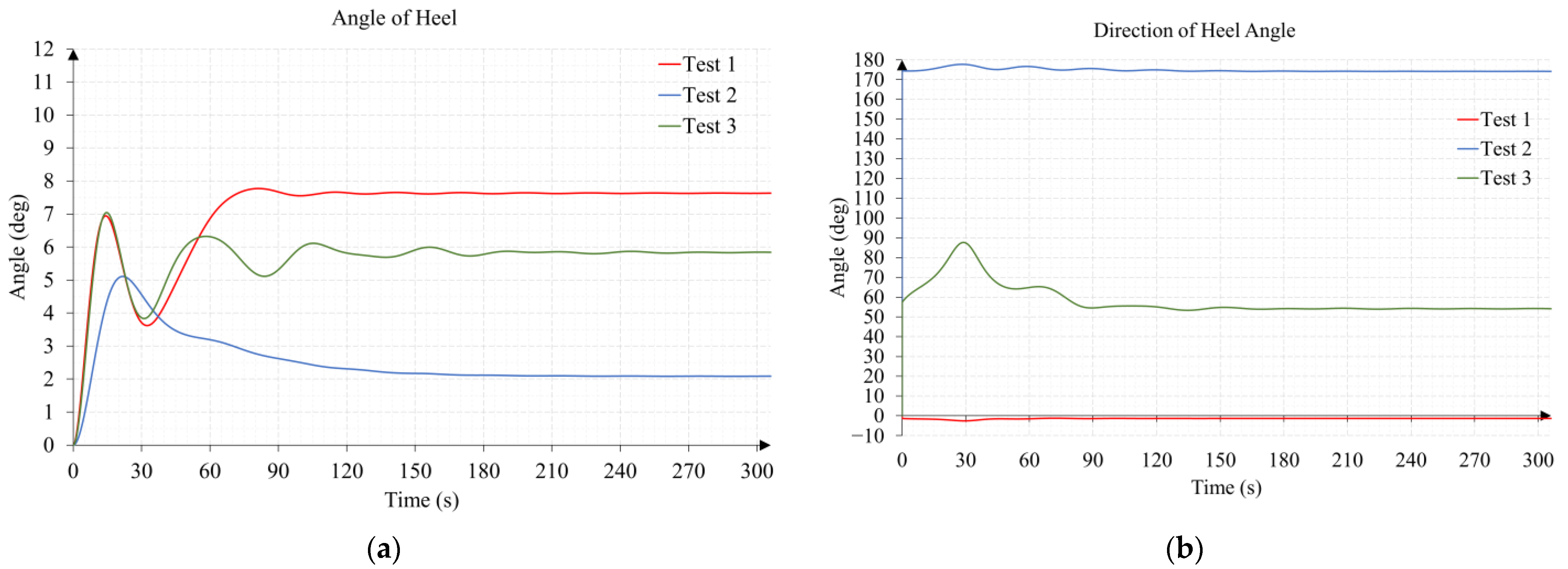
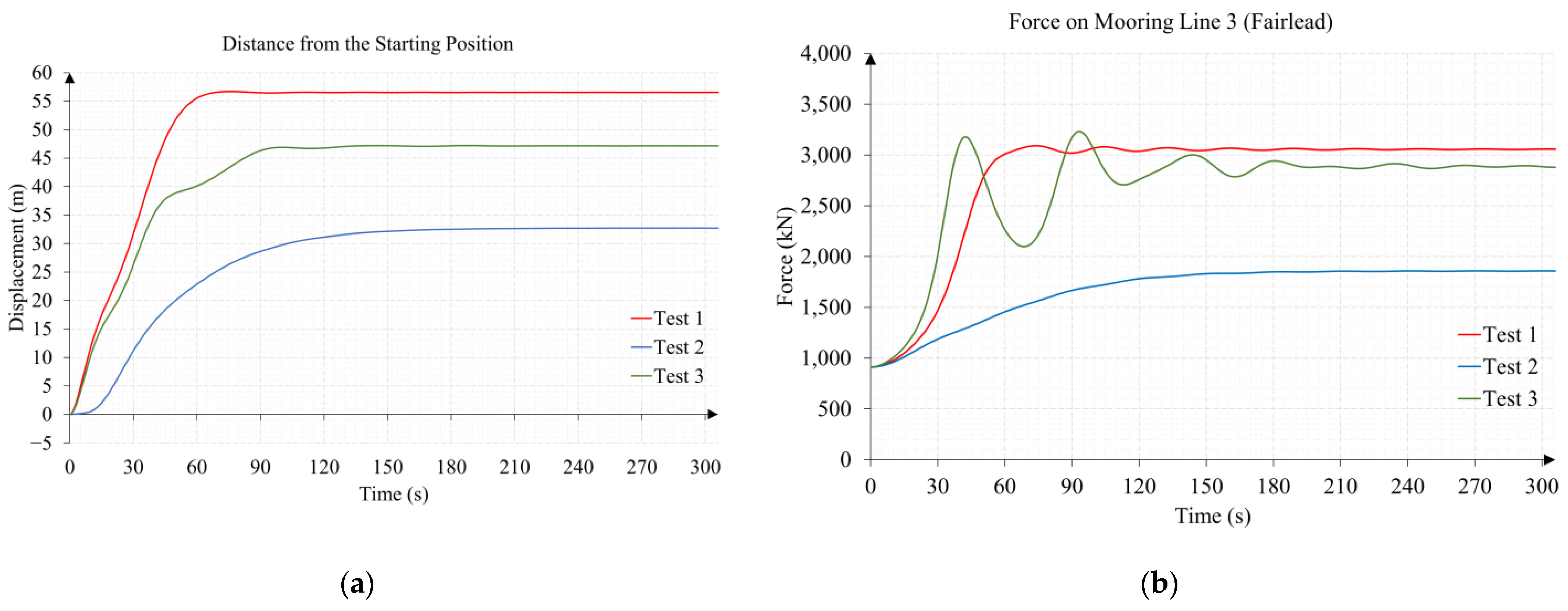
The main objective of the development of the mathematical model is to analyze the stability and energy production of the floating system under different conditions to develop automatic control strategies that improve the behavior of the system, from the point of view of structural fatigue and the maximum energy generation.
In this paper, a large part of the developed mathematical model is explained, leaving for the second part of this paper the detailed exposition of the modeling of the influencing forces on the floating hybrid system. The modeling techniques explained in this work allow us to obtain, in a simple way, the modeling of any mechanical system. This is of great help in control engineering when reliable modeling is needed without going too deep into the mechanical analysis.
The results presented in Section 3 were obtained by applying the one-dimensional theory to model the thrust of wind and marine current turbines. In the second part of this paper, the modeling of turbines using One-dimensional theory and Blade element momentum theory will also be explained. The Blade element momentum theory will permit the evaluation of the floating hybrid system applying different geometries, aerodynamic airfoils, including or eliminating certain elements, etc., also thanks to the availability of the inertial characteristics of the single bodies that make up the floating system (Appendix A) and a simple procedure (explained in Section 2.3.2) to process these characteristics and obtain the global inertia tensor of the system.
Therefore, the tests carried out in Section 3 represent the natural behavior of the floating system when it is subjected to the action of the wind and the marine current, without an integrated control system working to minimize structural stress while maximizing energy production. In future work, these control strategies and the results obtained will be exposed.
The programming of the FHYGSYS was conducted in Matlab® as it is an environment oriented to matrix calculation, although it could have been conducted with any other programming language that would allow a similar ease of matrix calculation. The programming was organized applying the clean code techniques exposed in [79]. Without the application of these programming techniques, the realization of FHYGSYS would have been much more complicated.
From the analysis of the tests carried out in Section 3, it follows that the smaller the angle of heel, the greater the energy production. As this is the main objective of the floating hybrid system, the control system will have to use the angle of heel as the main variable that it will have to minimize. The orientation of the wind and the marine current should also be considered to sacrifice energy production, if necessary, when the hybrid system approaches the worst-case situation described in the previous section. In this sense, the set of turbines can work in active stabilization mode to help, as a cooperative control, for the stabilization of the system. Regarding the possibilities of actuation, the torque of the turbines must also be considered—which can be controlled for low fluid speeds—and the pitch angle that can be used in any range of fluid speeds.
As a complement to the control system, to help increase the stability of the floating hybrid system, the possibility of increasing the mooring lines can be considered.
As future work in a forthcoming publication, cooperative control techniques that make compatible the achievement of maximum structural stability and optimal performance of the generation of the floating system will be addressed.
While the proposed model uses a horizontal WT, using a vertical WT is a possibility that could be explored in the future. In terms of power generation, horizontal WT works better [80], and it is more efficient because there are few wind angle changes. This is the most probable scenario in the locations described in the introduction with high wind speed and high marine currents. On the other hand, vertical WT has half the weight for the same power, which is an advantage for stability, and it works better with the wind changing directions. Future works will explore the use of vertical WTs in order to test the benefits of this kind of turbine.

Supplementary Materials

The following supporting information can be downloaded at: https://www.mdpi.com/article/10.3390/jmse11010126/s1, Video S1: Test_1; Video S2: Test_2; Video S3: Test_3.

Author Contributions

Conceptualization, E.G.; methodology, F.T and E.G.; software, F.T.; validation, F.T., E.G., A.C. and E.Q.; formal analysis, F.T., E.G. and E.Q.; investigation, E.G., E.Q., A.C. and F.T.; resources, E.G., F.T. and A.C.; data curation, F.T., E.G., E.Q. and A.C.; writing—original draft preparation, F.T. and E.G.; writing—review and editing, F.T., E.G., E.Q. and A.C.; visualization, E.G., F.T. and E.Q.; supervision, E.G., E.Q. and A.C.; project administration, E.G., E.Q and A.C.; funding acquisition, E.G. and E.Q. All authors have read and agreed to the published version of the manuscript.

Funding

This research received no external funding.

Institutional Review Board Statement

Not applicable.

Data Availability Statement

Not applicable.

Conflicts of Interest

The authors declare no conflict of interest.

Appendix A

In this Appendix, the individual inertial characteristics of the single bodies that make up the floating hybrid system are shown. The centers of mass and the moments and products of inertia given in this appendix are expressed in the mobile coordinate system.
Table A1. Inertial properties of the floating system.
ElementFloating Hybrid System
Density (kg/m3)-
Mass (kg)8,138,259
Ixx (kg·m2)67,434,701,761
Iyy (kg·m2)67,398,679,463
Izz (kg·m2)144,576,159
Ixy (kg·m2)7.56248
Iyz (kg·m2)−75.8696
Izx (kg·m2)−12,699,829
Center of Mass
Surge (m)−0.0172219
Sway (m)0
Heave (m)−76.6108
Table A1 shows the global inertial characteristics of the floating hybrid system, while Table A2 includes the global inertial characteristics of the submerged volume.
Table A2. Inertial properties of the floating system to calculate added mass.
ElementFloating Hybrid System
Density (kg/m3)1025
Volume (m3)8100.42
Mass (kg)8,302,931
Ixx (kg·m2)41,051,048,910
Iyy (kg·m2)41,036,448,653
Izz (kg·m2)103,989,376
Ixy (kg·m2)0
Iyz (kg·m2)0
Izx (kg·m2)−60,847.1
Center of Buoyancy
Surge (m)0.000366417
Sway (m)0
Heave (m)−61.6897
The moments and products of inertia are calculated at the center of mass—or center of buoyancy—in all Tables that appear in this Appendix except Table A1 and Table A2. In these two tables, these are calculated at the origin of the mobile coordinate system.

Appendix A.1. Inertial Properties of the Floating Platform and Ballast

The floating platform (Figure A1a) was designed with steel plate of the same density as that used for the tower in [81] and with the dimensions indicated in [31]. It is a hollow solid with a thickness of 35 mm of steel sheet. The ballast (Figure A1b) was designed as a solid cylinder with a density similar to that of concrete. The inertial characteristics of the platform-ballast set (Figure A1c) are adjusted to those of the floating platform described in [31]. Table A3 shows the inertial characteristics of the floating platform, the ballast and the platform-ballast set. Table A4 shows the inertial characteristics of the submerged volume of the floating platform.
Figure A1. (a) Floating platform; (b) ballast; (c) floating platform and ballast.
Jmse 11 00126 g0a1
Table A3. Inertial properties of the floating platform and ballast.
ElementFloating PlatformBallastFloating Platform, Including Ballast
Density (kg/m3)85001900-
Mass (kg)1,120,0306,217,3057,337,335
Ixx (kg·m2)1,578,897,2071,220,718,8514,171,601,865
Iyy (kg·m2)1,578,897,2071,220,718,8514,171,601,865
Izz (kg·m2)22,855,28067,651,19290,506,471
Ixy (kg·m2)000
Iyz (kg·m2)000
Izx (kg·m2)000
Center of Mass
Surge (m)000
Sway (m)000
Heave (m)−58.0124−96.0338−90.2299
Table A4. Inertial properties of the floating platform to calculate added mass.
ElementFloating Platform
Density (kg/m3)1025
Volume (m3)8029.2092
Mass (kg)8,229,939
Ixx (kg·m2)9,305,500,326
Iyy (kg·m2)9,305,500,326
Izz (kg·m2)89,000,314
Ixy (kg·m2)0
Iyz (kg·m2)0
Izx (kg·m2)0
Center of Buoyancy
Surge (m)0
Sway (m)0
Heave (m)−62.0657

Appendix A.2. Inertial Properties of the Tower

The tower (Figure A2) was designed with steel plate of the same density as that used for the tower in [81] and with the dimensions indicated in [50]. Table A5 shows the inertial characteristics of the tower.
Figure A2. Tower.
Figure A2. Tower.
Jmse 11 00126 g0a2
Table A5. Inertial properties of the tower.
ElementTower
Density (kg/m3)8500
Mass (kg)249,646
Ixx (kg·m2)120,213,483
Iyy (kg·m2)120,213,483
Izz (kg·m2)1,817,968
Ixy (kg·m2)0
Iyz (kg·m2)0
Izx (kg·m2)0
Center of Mass
Surge (m)0
Sway (m)0
Heave (m)43.3463

Appendix A.3. Inertial Properties of the Nacelle

The nacelle (Figure A3) was designed with the dimensions indicated in [50]. Table A6 shows the inertial characteristics of the nacelle.
Figure A3. Nacelle.
Figure A3. Nacelle.
Jmse 11 00126 g0a3
Table A6. Inertial properties of the nacelle.
ElementNacelle
Density (kg/m3)8492
Mass (kg)240,001
Ixx (kg·m2)474,602
Iyy (kg·m2)2,644,018
Izz (kg·m2)2,600,981
Ixy (kg·m2)0
Iyz (kg·m2)0
Izx (kg·m2)−293,804
Center of Mass
Surge (m)1.90642
Sway (m)0
Heave (m)89.3523

Appendix A.4. Inertial Properties of the Wind Hub

Table A7 shows the inertial characteristics of the wind hub, the first column shows the moments and products of inertia oriented with the local coordinate system (Figure A4) and the second column, oriented respect to the mobile coordinate system. The center of mass is expressed in each of the coordinate systems depending on the case.
The wind hub was designed to place the blades in the position indicated in [50], including the precone angle. In the design, the inertial characteristics of the hub defined in [50] were considered, and it has been tried to approximate them as much as possible.
Figure A4. Wind hub and local wind hub coordinate system.
Jmse 11 00126 g0a4
Table A7. Inertial properties of the wind hub.
ElementWind Hub (Values Expressed in Local Coordinate System)Wind Hub
Density (kg/m3)66776677
Mass (kg)56,781.956,781.9
Ixx (kg·m2)186,851188,149
Iyy (kg·m2)357,732357,732
Izz (kg·m2)357,732356,434
Ixy (kg·m2)00
Iyz (kg·m2)00
Izx (kg·m2)0−14,836.6
Center of Mass
Surge (m)−2.28302−5.00102
Sway (m)00
Heave (m)090.0001

Appendix A.5. Inertial Properties of the Wind Blade

Table A8 shows the inertial characteristics of the wind blade, the first column shows the moments and products of inertia oriented with the local coordinate system (Figure A5) and the other three columns, oriented respect to the mobile coordinate system. The center of mass is expressed in each of the coordinate systems depending on the case.
The blade was designed as a succession of aerodynamic profiles of different widths, according to the blade aerodynamic properties indicated in [50]. It is a hollow solid with an average thickness of approximately 20 mm. The airfoils used in the design will be found in [82], in a file called “DOWEC-NREL 5MW blade airfoil data-v2.xls”.
Figure A5. Wind blade and local wind blade coordinate system.
Jmse 11 00126 g0a5
Table A8. Inertial properties of the wind blade.
ElementWind Blade (Values Expressed in Local Coordinate System)Blade 1Blade 2Blade 3
Density (kg/m3)599.55599.55599.55599.55
Mass (kg)17,740.217,740.217,740.217,740.2
Ixx (kg·m2)3,118,0063,108,9943,100,3283,101,268
Iyy (kg·m2)3,106,3023,106,302800,161803,206
Izz (kg·m2)30,740.439,751.72,354,5602,350,574
Ixy (kg·m2)3278.723346.11199,425−202,771
Iyz (kg·m2)1616.541471.991,317,325−1,318,797
Izx (kg·m2)35,997.0170,397118,667113,465
Center of Mass
Surge (m)0.0881023−4.14516−7.01647−7.01551
Sway (m)−0.00636023−0.00636023−19.014219.0205
Heave (m)20.4750111.96879.149379.1603

Appendix A.6. Inertial Properties of the Current Turbine Support

The current turbine support (Figure A6) was designed to position the marine current turbines at the same depth described in [32]. The central cylindrical part was designed with 50 mm of steel sheet. The arms that support the nacelles were designed with hollow tubes also made of 50 mm of steel sheet.
Table A9 shows the inertial characteristics of the current turbine support. Table A10 includes the inertial characteristics of the submerged volume of the current turbine support.
Figure A6. Current turbine support.
Jmse 11 00126 g0a6
Table A9. Inertial properties of the current turbine support.
ElementCurrent Turbine Support
Density (kg/m3)8500
Mass (kg)166,609
Ixx (kg·m2)18,671,885
Iyy (kg·m2)3,486,640
Izz (kg·m2)17,165,901
Ixy (kg·m2)0
Iyz (kg·m2)0
Izx (kg·m2)−119,798
Center of Mass
Surge (m)0.267219
Sway (m)0
Heave (m)−17.4604
Table A10. Inertial properties of the current turbine support to calculate added mass.
ElementCurrent Turbine Support
Density (kg/m3)1025
Volume (m3)48.2405
Mass (kg)49,446.5
Ixx (kg·m2)8,297,263
Iyy (kg·m2)540,739
Izz (kg·m2)8,051,828
Ixy (kg·m2)0
Iyz (kg·m2)0
Izx (kg·m2)−28,822.1
Center of Buoyancy
Surge (m)0.556,826
Sway (m)0
Heave (m)−18.9532

Appendix A.7. Inertial Properties of the Marine Current Hub

Table A11 and Table A12 show the inertial characteristics of the marine current hub, the first column of each table shows the moments and products of inertia oriented with the local coordinate system (Figure A7) and the other two columns, oriented respect to the mobile coordinate system. The center of mass—or center of buoyancy—is expressed in each of the coordinate systems depending on the case. Table A12 includes the inertial characteristics of the submerged volume of the marine current hub.
Figure A7. Marine current hub and local marine current hub coordinate system.
Jmse 11 00126 g0a7
Table A11. Inertial properties of the marine current hub.
ElementMarine Current Hub (Values Expressed in Local Coordinate System)Clockwise HubCounterclockwise Hub
Density (kg/m3)850085008500
Mass (kg)10,906.110,906.110,906.1
Ixx (kg·m2)9399.479399.479399.47
Iyy (kg·m2)10,295.110,295.110,295.1
Izz (kg·m2)10,536.510,536.510,536.5
Ixy (kg·m2)000
Iyz (kg·m2)000
Izx (kg·m2)000
Center of Mass
Surge (m)−1.26718−1.06718−1.06718
Sway (m)017.1−17.1
Heave (m)0−20−20
Table A12. Inertial properties of the marine current hub to calculate added mass.
ElementMarine Current Hub (Values Expressed in Local Coordinate System)Clockwise HubCounterclockwise Hub
Density (kg/m3)102510251025
Volume (m3)7.413927.413927.41392
Mass (kg)7599.277599.277599.27
Ixx (kg·m2)3983.293983.293983.29
Iyy (kg·m2)4830.214830.214830.21
Izz (kg·m2)4949.324949.324949.32
Ixy (kg·m2)000
Iyz (kg·m2)000
Izx (kg·m2)000
Center of Buoyancy
Surge (m)−1.27678−1.07678−1.07678
Sway (m)017.1−17.1
Heave (m)0−20−20

Appendix A.8. Inertial Properties of the Marine Current Blades

Table A13 and Table A14 show the inertial characteristics of the clockwise marine current blades, while Table A15 and Table A16 include those of the counterclockwise blades. The first column of each table shows the moments and products of inertia oriented with the local coordinate system (Figure A8) and the other two columns, oriented respect to the mobile coordinate system. The center of mass—or center of buoyancy—is expressed in each of the coordinate systems depending on the case.
The blades were designed as a succession of hydrodynamic profiles of different widths, according to the blade hydrodynamic properties indicated in [32]. It was modeled as a solid body. According to [32], only one hydrofoil has been used in the blade design. The hydrofoil—NACA 63-424—was obtained using the GNacaLt V0.1.0 software [83].
Figure A8. Marine current blade and local marine current blade coordinate system: (a) clockwise blade; (b) counterclockwise blade.
Jmse 11 00126 g0a8
Table A13. Inertial properties of the clockwise marine current blade.
ElementClockwise Blade (Values Expressed in Local Coordinate System)Blade 1Blade 2
Density (kg/m3)157815781578
Mass (kg)3213.433213.433213.43
Ixx (kg·m2)15,720.115,720.115,720.1
Iyy (kg·m2)15,493.915,493.915,493.9
Izz (kg·m2)298.420298.420298.420
Ixy (kg·m2)44.742644.7426−44.7426
Iyz (kg·m2)77.048777.048777.0487
Izx (kg·m2)124.715124.715−124.715
Center of Mass
Surge (m)−0.0731756−0.973176−0.973176
Sway (m)−0.10580116.994217.2058
Heave (m)3.46741−15.5326−24.4674
Table A14. Inertial properties of the clockwise marine current blade to calculate added mass.
ElementClockwise Blade (Values Expressed in Local Coordinate System)Blade 1Blade 2
Density (kg/m3)102510251025
Volume (m3)2.036402.036402.03640
Mass (kg)2087.312087.312087.31
Ixx (kg·m2)10,211.110,211.110211.1
Iyy (kg·m2)10,064.210,064.210,064.2
Izz (kg·m2)193.840193.840193.840
Ixy (kg·m2)29.062829.0628−29.0628
Iyz (kg·m2)50.047550.047550.0475
Izx (kg·m2)81.009681.0096−81.0096
Center of Buoyancy
Surge (m)−0.0731756−0.973176−0.973176
Sway (m)−0.10580116.994217.2058
Heave (m)3.46741−15.5326−24.4674
Table A15. Inertial properties of the counterclockwise marine current blade.
ElementCounterclockwise Blade (Values Expressed in Local Coordinate System)Blade 1Blade 2
Density (kg/m3)157815781578
Mass (kg)3213.433213.433213.43
Ixx (kg·m2)15,720.115,720.115,720.1
Iyy (kg·m2)15,493.915,493.915,493.9
Izz (kg·m2)298.420298.420298.420
Ixy (kg·m2)−44.7426−44.742644.7426
Iyz (kg·m2)−77.0487−77.0487−77.0487
Izx (kg·m2)124.715124.715−124.715
Center of Mass
Surge (m)−0.0731756−0.973176−0.973176
Sway (m)0.105801−16.9942−17.2058
Heave (m)3.46741−15.5326−24.4674
Table A16. Inertial properties of the counterclockwise marine current blade to calculate added mass.
ElementCounterclockwise Blade (Values Expressed in Local Coordinate System)Blade 1Blade 2
Density (kg/m3)102510251025
Volume (m3)2.036402.036402.03640
Mass (kg)2087.312087.312087.31
Ixx (kg·m2)10,211.110,211.110,211.1
Iyy (kg·m2)10,064.210,064.210,064.2
Izz (kg·m2)193.840193.840193.840
Ixy (kg·m2)−29.0628−29.062829.0628
Iyz (kg·m2)−50.0475−50.0475−50.0475
Izx (kg·m2)81.009681.0096−81.0096
Center of Buoyancy
Surge (m)−0.0731756−0.973176−0.973176
Sway (m)0.105801−16.9942−17.2058
Heave (m)3.46741−15.5326−24.4674

Appendix B

This appendix shows, as an example, the necessary rotations of the wind blade inertia tensor to align it with the mobile coordinate system. This operation is performed for all three blades. Table A17 shows the values of the angles that the inertia tensor is going to be rotate. The angles between the blades, the precone angle and the shaft tilt angle are fixed values taken from [50]. The azimuth angle is the angular position of the wind turbine axis, and the nacelle yaw angle is the rotation made by the nacelle to orient itself in the direction of the wind—if the floating system is in its initial position, these two values are zero.
Table A17. Necessary rotations for the alignment of the inertia tensor of the wind turbine blades.
DescriptionValue (Degrees)Symbol
Precone angle−2.5 φ 1
Angle between blades *0, 120, 240 φ 2
Azimuth angle0 φ 3
Shaft tilt angle5 φ 4
Nacelle yaw angle0 φ 5
* Values of blades 1, 2 and 3.
In this example, all rotations of the inertia tensor are performed at once. In (A1,A2), the rotation matrix containing all the desired rotations of the inertia tensor. With this matrix, applying (A3) the unit vectors oriented towards the desired final direction are obtained.
M I T R O T = M r o t Y ( φ 1 ) · M r o t X ( φ 2 ) · M r o t X ( φ 3 ) · M r o t Y ( φ 4 ) · M r o t Z ( φ 5 )
M I T R O T = cos φ 1 0 sin φ 1 0 1 0 sin φ 1 0 cos φ 1 · 1 0 0 0 cos φ 2 sin φ 2 0 sin φ 2 cos φ 2 · 1 0 0 0 cos φ 3 sin φ 3 0 sin φ 3 cos φ 3 · cos φ 4 0 sin φ 4 0 1 0 sin φ 4 0 cos φ 4 · cos φ 5 sin φ 5 0 sin φ 5 cos φ 5 0 0 0 1
[ u 1 v 1 w 1 u 2 v 2 w 2 u 3 v 3 w 3 ] = M I T R O T · [ 1 0 0 0 1 0 0 0 1 ]
Through Equation (8) the inertia tensor of the wind blade—first column of Table A8—is prepared, then Equations (12) and (13) is applied with the unit vectors obtained with Equation (A3). With this operation, the inertia tensors of the last three columns of Table A8 are calculated by choosing an angle between blades, 0, 120 or 240 degrees, respectively.

Appendix C

Since the mathematical model bases its operation on fundamental operations such as differentiation and integration, methods must be used that allow these operations to be carried out with an acceptable margin of error. These operations are performed with respect to the time differential used for the simulation, so numerical differentiation and integration techniques must be used.
Different differentiation methods were tested and, using procedures less precise than that indicated in Appendix C.1, the results have not been considered acceptable.
Regarding the integration method, applying what is explained in Appendix C.2, better results are obtained, for the same time differential, than using simpler methods such as the trapezoidal rule. This allows us to obtain results with an acceptable error with a time difference of 0.1 s.

Appendix C.1. Numerical Differentiation Method of Richardson’s Extrapolation

It is initially based on the expansion of the Taylor series backwards to the third derivative term Equation (A4) [69].
f ( x i 1 ) = f ( x i ) f ( x i ) · Δ t + f ( x i ) 2 ! · Δ t 2 f ( x i ) 3 ! · Δ t 3
The terms of the second and third derivatives of (A4) are replaced by the backward finite divided difference Formulas (A5) and (A6) [69]. Where xi and xi-i are the value of the function to be derived at the current and previous times, respectively, and Δ t the value of the time increment in which the mathematical model is evaluated.
f ( x i ) = 2 · f ( x i ) 5 · f ( x i 1 ) + 4 · f ( x i 2 ) f ( x i 3 ) Δ t 2
f ( x i ) = 5 · f ( x i ) 18 · f ( x i 1 ) + 24 · f ( x i 2 ) 14 · f ( x i 3 ) + 3 · f ( x i 4 ) 2 · Δ t 3
Combining (A4)–(A6) gives an estimate of the derivative (A7) with an error O(h2) [69].
f ( x i ) = 19 · f ( x i ) 24 · f ( x i 1 ) + 8 · f ( x i 3 ) 3 · f ( x i 4 ) 12 · Δ t = D ( Δ t )
Expressing (A7) for a double time differential gives (A8).
D ( 2 Δ t ) = 19 · f ( x i ) 24 · f ( x i 2 ) + 8 · f ( x i 6 ) 3 · f ( x i 8 ) 24 · Δ t
Applying the expression of Richardson’s extrapolation (A9) [69], an estimation of the derivative with error O(h4) is obtained.
D R E   1 = 4 3 · D ( Δ t ) 1 3 · D ( 2 Δ t )
Recursively applying Richardson’s extrapolation (A10)–(A12) [69], an estimate of the derivative with error O(h6) is obtained.
D ( 4 Δ t ) = 19 · f ( x i ) 24 · f ( x i 4 ) + 8 · f ( x i 12 ) 3 · f ( x i 16 ) 48 · Δ t
D R E   2 = 4 3 · D ( 2 Δ t ) 1 3 · D ( 4 Δ t )
D i = 16 15 · D R E   1 1 15 · D R E   2
If more precision is desired, Richardson’s extrapolation can still be applied recursively.

Appendix C.2. Numerical Integration Method of Romberg’s Algorithm

The integration method of Romberg’s algorithm is based on the iterative application of Richardson’s extrapolation, similar to how it is conducted in numerical differentiation [69]. For this, the multiple application trapezoidal rule (A13)–(A15) is initially applied [69].
I ( Δ t ) = Δ t · f ( x i ) + f ( x i 1 ) 2
I ( 2 Δ t ) = Δ t · f ( x i ) + 2 · f ( x i 1 ) + f ( x i 2 ) 4
I ( 4 Δ t ) = Δ t · f ( x i ) + 2 · ( f ( x i 1 ) + f ( x i 2 ) + f ( x i 3 ) ) + f ( x i 4 ) 8
Equations (A13)–(A15) have an error O(h2), combining them through (A16) and (A17), approximations of the integral with error O(h4) are obtained [69].
I R E   1 = 4 3 · I ( Δ t ) 1 3 · I ( 2 Δ t )
I R E   2 = 4 3 · I ( 2 Δ t ) 1 3 · I ( 4 Δ t )
I i = I ( i 1 ) + 16 15 · I R E   1 1 15 · I R E   2
Finally, Equations (A16) and (A17) are combined using Equation (A18) obtaining an error O(h6) [69]. To obtain the result of the integral over time, the value of the integral at the previous instant (I(i-1)) is added at each instant of time. As in the case of differentiation, if more precision is desired, Richardson’s extrapolation can still be applied recursively.

Appendix D

Appendix D.1. Calculation of Heel Angle

It is obtained by calculating the scalar product [84] of the unit vectors in the heave direction of the inertial ( v h i ) and mobile ( v h m ) coordinate systems Equation (A19). Both vectors expressed in the inertial coordinate system.
φ h e e l = acos ( v h i x · v h m x + v h i y · v h m y + v h i z · v h m z | v h i | · | v h m | )

Appendix D.2. Calculation of the Direction of Heel Angle

It is obtained by calculating the scalar product [84] of the unit vector in the surge direction of the inertial coordinate system ( v s i ) and another vector ( v h o m ) whose x and y components are those of the unit vector in the heave direction of the mobile coordinate system and the z component is equal to zero Equation (A20). Both vectors expressed in the inertial coordinate system.
φ h e e l d i r = acos ( v s i x · v h o m x + v s i y · v h o m y + v s i z · v h o m z | v s i | · | v h o m | )

Appendix E

In this appendix, the validation carried out for the mathematical model is exposed. The validation was made from simulations obtained with FAST8 that were compared with simulations, under the same conditions, obtained with FHYGSYS. Comparisons were made for many situations; in this appendix, four representative situations have been selected that allow us to infer the behavior of FHYGSYS.
To compare the results with FAST8, the model of a floating system equivalent to the one shown in Figure 2 was used, but without including the marine current turbines, that is, an OC3-Hywind model [31] (Figure A9).
Figure A9. OC3-Hywind Model used to Test the Validation.
Jmse 11 00126 g0a9
To compose the model, the inertial characteristics of the floating platform (Table A3 and Table A4), of the tower (Table A5), of the nacelle (Table A6), of the hub (Table A7), and of the blades (Table A8) were used.
To complete the modeling of the OC3-Hywind system, it is necessary to use a ballast with different characteristics from those indicated in Table A3. This is to match the inertial characteristics of the floating platform-ballast set with those indicated in [31].
In fact, this was conducted prior to the ballast design of the floating hybrid system described in Figure 2, since validation was the first task performed before incorporating the tidal current turbines into the OC3-Hywind system. The inertial characteristics of the ballast used are shown in Table A18.
Table A18. Inertial properties of the ballast to model an OC3-Hywind floating system.
ElementBallast
Density (kg/m3)1900
Mass (kg)6,345,580
Ixx (kg·m2)1,296,406,888
Iyy (kg·m2)1,296,406,888
Izz (kg·m2)69,046,972
Ixy (kg·m2)0
Iyz (kg·m2)0
Izx (kg·m2)0
Center of Mass
Surge (m)0
Sway (m)0
Heave (m)−95.54
Putting together all the indicated elements that make up the OC3-Hywind floating system, the global inertial characteristics are obtained, these are shown in Table A19 and Table A20.
Table A19. Inertial properties of the OC3-Hywind floating system.
ElementHybrid Floating System
Density (kg/m3)-
Mass (kg)8,065,259
Ixx (kg·m2)67,999,304,954
Iyy (kg·m2)67,988,554,932
Izz (kg·m2)118,598,012
Ixy (kg·m2)0
Iyz (kg·m2)0
Izx (kg·m2)−12,518,376
Center of Mass
Surge (m)−0.0184607
Sway (m)0
Heave (m)−77.9964
Table A20. Inertial properties of the OC3-Hywind floating system to calculate added mass.
ElementHybrid Floating System
Density (kg/m3)1025
Volume (m3)8029.21
Mass (kg)8,229,939
Ixx (kg·m2)41,008,424,912
Iyy (kg·m2)41,008,424,912
Izz (kg·m2)89,000,314
Ixy (kg·m2)0
Iyz (kg·m2)0
Izx (kg·m2)0
Center of Buoyancy
Surge (m)0
Sway (m)0
Heave (m)−62.0657
Four cases were chosen to validate the mathematical model: one with only wind, another with only sea current, and two in which both wind and sea current with different inclination are combined. Table A21 shows the characteristics of the four mentioned tests.
Table A21. Validation tests.
TestWind SpeedWind DirectionMarine Current SpeedMarine Current Direction
Test V01001.9 m/s280 deg
Test V0211 m/s110 deg00
Test V0311 m/s70 deg1.9 m/s70 deg
Test V0411 m/s200 deg1.9 m/s70 deg
For the validation process, the FAST8 software was downloaded from [85] and was configured once downloaded as follows:
The files “Test24.fst” and “Test24.cru” are copied from the “/CertTest” directory to the “/bin” directory.
The directory “5MW_Baseline” is copied from “/CertTest” to “/bin”.
The “Test24.fst” file is edited and modified as indicated in Table A22. This file contains the configuration for the simulation of the Floating OC3 system.
Table A22. Changes in “Test24.fst”.
SectionParameterOriginal ValueModified Value
SIMULATION CONTROLTMax60300
OUTPUTOutFileFmt23
The “NRELOffshrBsline5MW_OC3Hywind_ElastoDyn.dat” file is edited and modified as indicated in Table A23. This disables the flexible behavior of both the blades and the tower.
Table A23. Changes in “NRELOffshrBsline5MW_OC3Hywind_ElastoDyn.dat”.
SectionParameterOriginal ValueModified Value
DEGREES OF FREEDOMFlapDOF1TrueFalse
FlapDOF2TrueFalse
EdgeDOFTrueFalse
DrTrDOFTrueFalse
YawDOFTrueFalse
TwFADOF1TrueFalse
TwFADOF2TrueFalse
TwSSDOF1TrueFalse
TwSSDOF2TrueFalse
INITIAL
CONDITIONS
RotSpeed12.111.89
The “NRELOffshrBsline5MW_InflowWind_12mps.dat” file is edited and modified as indicated in Table A24. A value of power law exponent of 1/7 is chosen as indicated in [74].
Table A24. Changes in “NRELOffshrBsline5MW_InflowWind_12mps.dat”.
SectionParameterOriginal ValueModified Value
WindType31
Parameters for Steady Wind ConditionsHWindSpeed011
PLexp0.20.142857
The “NRELOffshrBsline5MW_OC3Hywind_AeroDyn15.dat” file is edited and modified as indicated in Table A25. In [86], it is indicated that if the wind turbine is not parked or idling, TwrAero must be equal to FALSE.
Table A25. Changes in “NRELOffshrBsline5MW_OC3Hywind_AeroDyn15.dat”.
SectionParameterOriginal ValueModified Value
General OptionsAFAeroMod21
TwrAeroTrueFalse
The “NRELOffshrBsline5MW_OC3Hywind_HydroDyn.dat” file is edited and modified as indicated in Table A26. Wave action is disconnected to facilitate the validation of the mathematical model. In the second part of this paper, validation results will be shown with the improved mathematical model incorporating wave action.
Table A26. Changes in “NRELOffshrBsline5MW_OC3Hywind_HydroDyn.dat”.
SectionParameterOriginal ValueModified Value
WAVESWaveMod20
In order to represent the magnitudes necessary to make the comparison between FAST and FHYGSYS, it is necessary to obtain the response of more magnitudes than those offered by default in test 24. Table A27 and Table A28 indicate the magnitudes to be included in the corresponding file.
Table A27. Inclusion in “NRELOffshrBsline5MW_OC3Hywind_AeroDyn15.dat”—OutList section—new output parameters.
ParameterDescriptionUnits
RtAeroFxhTotal rotor aerodynamic load(force in x, y and z directions)(N)
RtAeroFyh(N)
RtAeroFzh(N)
RtAeroMxhTotal rotor aerodynamic load(moment in x, y and z directions)(N·m)
RtAeroMyh(N·m)
RtAeroMzh(N·m)
RtTSRRotor tip-speed ratio(-)
RtAeroCpRotor aerodynamic power coefficient(-)
RtAeroCtRotor aerodynamic coefficient(-)
Table A28. Inclusion in “NRELOffshrBsline5MW_OC3Hywind_HydroDyn.dat”—OutList section—new output parameters.
ParameterDescriptionUnits
HydroFxiTotal integrated hydrodynamic load from both potential flow and strip theory at the WRP (force in x, y, z directions)(N)
HydroFyi(N)
HydroFzi(N)
HydroMxiTotal integrated hydrodynamic load from both potential flow and strip theory at the WRP (moment in x, y, z directions)(N·m)
HydroMyi(N·m)
HydroMzi(N·m)
AddFxiForces and moments due to additional preload, stiffness, and damping at the WRP (force in x, y, z directions)(N)
AddFyi(N)
AddFzi(N)
AddMxiForces and moments due to additional preload, stiffness, and damping at the WRP (moment in x, y, z directions)(N·m)
AddMyi(N·m)
AddMzi(N·m)
HdrStcFxiHydrostatic loads at the WRP(force in x, y, z directions)(N)
HdrStcFyi(N)
HdrStcFzi(N)
HdrStcMxiHydrostatic loads at the WRP(moment in x, y, z directions)(N·m)
HdrStcMyi(N·m)
HdrStcMzi(N·m)
RdtnFxiRadiation loads at the WRP(force in x, y, z directions)(N)
RdtnFyi(N)
RdtnFzi(N)
RdtnMxiRadiation loads at the WRP(moment in x, y, z directions)(N·m)
RdtnMyi(N·m)
RdtnMzi(N·m)
FAST8 does not calculate the force and moment values of the viscous drag loads. In order to validate these forces obtained with FHYGSYS, Equations (A21) and (A22) is used. In this way the value of the forces resulting from the simulation with FAST8 is obtained indirectly from the data in Table A11.
V i s c D F j i = H y d r o F j i A d d F j i H d r S t c F j i R d t n F j i
V i s c D M j i = H y d r o M j i A d d M j i H d r S t c M j i R d t n M j i

Appendix E.1. Test V01 (Wind: 0 m/s—Marine Current: 1.9 m/s, 280 Degrees)

To carry out this test, the modifications indicated in Table A29 and Table A30 must be made in the corresponding files. Once the test is finished, the original values must be restored so as not to affect subsequent tests. In Table A30, −80 deg represents 280 deg.
Table A29. Changes in “Test24.fst”.
SectionParameterOriginal ValueModified Value
FEATURE SWITCHES AND FLAGSCompInflow10
CompAero20
Table A30. Changes in “NRELOffshrBsline5MW_OC3Hywind_HydroDyn.dat”.
SectionParameterOriginal ValueModified Value
CURRENTCurrMod01
CurrSSV001.9
CurrSSDir“DEFAULT”−80
Figure A10. Comparison of results between FAST8 and FHYGSYS, under Test V01 conditions: (a) linear degrees of freedom; (b) angular degrees of freedom; (c) total hydrodynamic loads, surge, and sway forces; (d) total hydrodynamic loads, surge, sway, and heave moments; (e) total hydrodynamic loads, heave force; (f) force in fairlead of each mooring line.
Jmse 11 00126 g0a10aJmse 11 00126 g0a10b
Figure A11. Comparison of results between FAST8 and FHYGSYS, under Test V01 conditions: (a) additional damping loads, surge, sway, and heave forces; (b) additional damping loads, surge, sway, and heave moments; (c) hydrostatic loads, surge, sway, and heave forces; (d) hydrostatic loads, surge, sway, and heave moments; (e) radiation loads, surge, sway, and heave forces; (f) radiation loads, surge, sway, and heave moments; (g) viscous drag loads, surge, sway, and heave forces; (h) viscous drag loads, surge, sway, and heave moments.
Jmse 11 00126 g0a11aJmse 11 00126 g0a11b

Appendix E.2. Test V02 (Wind: 11 m/s, 110 Degrees—Marine Current: 0 m/s)

To carry out this test, the modifications indicated in Table A31 and Table A32 must be made in the corresponding files. Once the test is finished, the original values must be restored so as not to affect subsequent tests.
Table A31. Changes in “NRELOffshrBsline5MW_OC3Hywind_ElastoDyn.dat”.
SectionParameterOriginal ValueModified Value
INITIAL
CONDITIONS
NacYaw0110
Table A32. Changes in “NRELOffshrBsline5MW_InflowWind_12mps.dat”.
SectionParameterOriginal ValueModified Value
PropagationDir0−110
Figure A12. Comparison of results between FAST8 and FHYGSYS, under Test V02 conditions: (a) linear degrees of freedom; (b) angular degrees of freedom; (c) total hydrodynamic loads, surge, and sway forces; (d) total hydrodynamic loads, surge, sway, and heave moments; (e) total hydrodynamic loads, heave force; (f) force in fairlead of each mooring line.
Jmse 11 00126 g0a12aJmse 11 00126 g0a12b
Figure A13. Comparison of results between FAST8 and FHYGSYS, under Test V02 conditions: (a) additional damping loads, surge, sway, and heave forces; (b) additional damping loads, surge, sway, and heave moments; (c) hydrostatic loads, surge, sway, and heave forces; (d) hydrostatic loads, surge, sway, and heave moments; (e) radiation loads, surge, sway, and heave forces; (f) radiation loads, surge, sway, and heave moments; (g) viscous drag loads, surge, sway, and heave forces; (h) viscous drag loads, surge, sway, and heave moments.
Jmse 11 00126 g0a13aJmse 11 00126 g0a13b
Figure A14. Comparison of results between FAST8 and FHYGSYS, under Test V02 conditions: (a) rotor thrust; (b) rotor torque; (c) generator torque; (d) electric power generation; (e) tip-speed ratio; (f) rotor speed; (g) power coefficient; (h) thrust coefficient.
Jmse 11 00126 g0a14aJmse 11 00126 g0a14b

Appendix E.3. Test V03 (Wind: 11 m/s, 70 Degrees—Marine Current: 1.9 m/s, 70 Degrees)

To carry out this test, the modifications indicated in Table A33, Table A34 and Table A35 must be made in the corresponding files. Once the test is finished, the original values must be restored so as not to affect subsequent tests.
Table A33. Changes in “NRELOffshrBsline5MW_OC3Hywind_ElastoDyn.dat”.
SectionParameterOriginal ValueModified Value
INITIAL
CONDITIONS
NacYaw070
Table A34. Changes in “NRELOffshrBsline5MW_InflowWind_12mps.dat”.
SectionParameterOriginal ValueModified Value
PropagationDir0−70
Table A35. Changes in “NRELOffshrBsline5MW_OC3Hywind_HydroDyn.dat”.
SectionParameterOriginal ValueModified Value
CURRENTCurrMod01
CurrSSV001.9
CurrSSDir“DEFAULT”70
Figure A15. Comparison of results between FAST8 and FHYGSYS, under Test V03 conditions: (a) linear degrees of freedom; (b) angular degrees of freedom; (c) total hydrodynamic loads, surge, and sway forces; (d) total hydrodynamic loads, surge, sway, and heave moments; (e) total hydrodynamic loads, heave force; (f) force in fairlead of each mooring line.
Jmse 11 00126 g0a15
Figure A16. Comparison of results between FAST8 and FHYGSYS, under Test V03 conditions: (a) additional damping loads, surge, sway, and heave forces; (b) additional damping loads, surge, sway, and heave moments; (c) hydrostatic loads, surge, sway, and heave forces; (d) hydrostatic loads, surge, sway, and heave moments; (e) radiation loads, surge, sway, and heave forces; (f) radiation loads, surge, sway, and heave moments; (g) viscous drag loads, surge, sway, and heave forces; (h) viscous drag loads, surge, sway, and heave moments.
Jmse 11 00126 g0a16
Figure A17. Comparison of results between FAST8 and FHYGSYS, under Test V03 conditions: (a) rotor thrust; (b) rotor torque; (c) generator torque; (d) electric power generation; (e) tip-speed ratio; (f) rotor speed; (g) power coefficient; (h) thrust coefficient.
Jmse 11 00126 g0a17

Appendix E.4. Test V03 (Wind: 11 m/s, 200 Degrees—Marine Current: 1.9 m/s, 70 Degrees)

To carry out this test, the modifications indicated in Table A36, Table A37 and Table A38 must be made in the corresponding files. Once the test is finished, the original values must be restored so as not to affect subsequent tests. In Table A36 −160 deg represents 200 deg.
Table A36. Changes in “NRELOffshrBsline5MW_OC3Hywind_ElastoDyn.dat”.
SectionParameterOriginal ValueModified Value
INITIAL
CONDITIONS
NacYaw0−160
Table A37. Changes in “NRELOffshrBsline5MW_InflowWind_12mps.dat”.
SectionParameterOriginal ValueModified Value
PropagationDir0−200
Table A38. Changes in “NRELOffshrBsline5MW_OC3Hywind_HydroDyn.dat”.
SectionParameterOriginal ValueModified Value
CURRENTCurrMod01
CurrSSV001.9
CurrSSDir“DEFAULT”70
Figure A18. Comparison of results between FAST8 and FHYGSYS, under Test V04 conditions: (a) linear degrees of freedom; (b) angular degrees of freedom; (c) total hydrodynamic loads, surge, and sway forces; (d) total hydrodynamic loads, surge, sway, and heave moments; (e) total hydrodynamic loads, heave force; (f) force in fairlead of each mooring line.
Jmse 11 00126 g0a18aJmse 11 00126 g0a18b
Figure A19. Comparison of results between FAST8 and FHYGSYS, under Test V04 conditions: (a) additional damping loads, surge, sway, and heave forces; (b) additional damping loads, surge, sway, and heave moments; (c) hydrostatic loads, surge, sway, and heave forces; (d) hydrostatic loads, surge, sway, and heave moments; (e) radiation loads, surge, sway, and heave forces; (f) radiation loads, surge, sway, and heave moments; (g) viscous drag loads, surge, sway, and heave forces; (h) viscous drag loads, surge, sway, and heave moments.
Jmse 11 00126 g0a19aJmse 11 00126 g0a19b
Figure A20. Comparison of results between FAST8 and FHYGSYS, under Test V04 conditions: (a) rotor thrust; (b) rotor torque; (c) generator torque; (d) electric power generation; (e) tip-speed ratio; (f) rotor speed; (g) power coefficient; (h) thrust coefficient.
Jmse 11 00126 g0a20aJmse 11 00126 g0a20b

Acronym

a,b,cshape parameters to define an ellipsoid
a v i   ( B O D Y ) acceleration vector of six degrees of freedom expressed in the mobile coordinate system
a v i   ( I N E R T I A L ) acceleration vector of six degrees of freedom expressed in the inertial coordinate system
α 0 , β 0 , γ 0 parameters which depend on the values of the semi-axes of the ellipsoid
CoBcenter of buoyancy of the floating system
CoBi center of buoyancy of submerged body i in the floating system
CoMcenter of mass of the floating system
CoMicenter of mass of body i in the floating system
CoRkcenter of rotation of the floating system on axis k, k ∈ (X, Y, Z)
eeccentricity of the meridian elliptical section
FHGS Floating Hybrid Generator System
FHYGSYS Floating Hybrid Generator Systems Simulator
FWT floating wind turbines
Ixx, Iyy, Izz, Ixy, Iyz, Izxmoments and products of inertia
itpvkinertia tensor position vector on axis k, k ∈ (x, y, z)
φLineiyaw angle with respect to inertial X axis of mooring line i
MAM added mass matrix
MCT marine current turbines
mFS total mass of the floating system
miindividual mass of body i in the floating system
MAMadded mass matrix of the floating system
MHT (t)the homogeneous matrix representing the necessary rotations and/or translations to place a point from its initial position to the one that occupies at each moment
MIT inertia tensor matrix of a body of the floating system
MIT (ROT)inertia tensor aligned with the mobile coordinate system
MIT (TRANS)inertia tensor translated to the origin of the mobile coordinate system
MIT (SUM) (FS)global inertia tensor of the submerged volume of the floating system
MIT (FS)global inertia tensor of the floating system
MRBrigid body matrix of the floating system
mSUM(t) mass of the submerged volume in the floating system
pBODY k point expressed in the mobile coordinate system on axis k, k ∈ (x, y, z)
pINERTIAL kpoint expressed in the inertial coordinate system on axis k, k ∈ (X, Y, Z)
qi system degree of freedom i
q i   ( I N E R T I A L ) position vector of six degrees of freedom expressed in the inertial coordinate system
pFi fairlead position of mooring line i
pAi anchor position of mooring line i
ρSEAWATERdensity of seawater
TRB kinetic energy that reaches the rigid body
TAM kinetic energy that reaches the added mass
Vi(t) submerged volume of each body in the floating system
VSUM(t) submerged volume of the floating system
v v i   ( B O D Y ) velocity vector of six degrees of freedom expressed in the mobile coordinate system
v v i   ( I N E R T I A L ) velocity vector of six degrees of freedom expressed in the inertial coordinate system
WT wind turbine
X u ˙ , Y v ˙ , Z w ˙ , K p ˙ , M q ˙ , N r ˙ moments and products of inertia of the submerged volume of the floating system corrected according to the shape of its volume

References

  1. García, E.; Correcher, A.; Quiles, E.; Morant, F. Renewable Energy Resources of the Marine Environment and Its Control Requirements. Rev. Iberoam. Autom. E Inform. Ind. 2016, 13, 141–161. [Google Scholar] [CrossRef] [Green Version]
  2. García, E.; Correcher, A.; Quiles, E.; Tamarit, F.; Morant, F. Control and Supervision Requirements for Floating Hybrid Generator Systems. Int. J. Environ. Res. Public Health 2022, 19, 12781. [Google Scholar] [CrossRef] [PubMed]
  3. Chen, H.; Tang, T.; Aït-Ahmed, N.; el Hachemi Benbouzid, M.; Machmoum, M.; El-Hadi Zaïm, M. Attraction, Challenge and Current Status of Marine Current Energy. IEEE Access 2018, 6, 12665–12685. [Google Scholar] [CrossRef]
  4. Zhou, Z.; Benbouzid, M.; Charpentier, J.F.; Scuiller, F.; Tang, T. Developments in Large Marine Current Turbine Technologies—A Review. Renew. Sustain. Energy Rev. 2017, 71, 852–858. [Google Scholar] [CrossRef]
  5. Ma, K.-T.; Luo, Y.; Kwan, T.; Wu, Y. Mooring for Floating Wind Turbines. In Mooring System Engineering for Offshore Structures; Elsevier: Amsterdam, The Netherlands, 2019; pp. 299–315. [Google Scholar] [CrossRef]
  6. WindFloat Concept. 2022. Available online: https://www.principlepower.com/windfloat (accessed on 28 November 2022).
  7. Windplus Consortium. 2015. Available online: https://www.power-technology.com/news/newswindplus-consortium-build-floating-wind-farm-offshore-portugal-4728781 (accessed on 28 November 2022).
  8. RWE Projects. 2022. Available online: https://www.rwe.com/en/research-and-development/wind-power/floating-offshore-wind (accessed on 28 November 2022).
  9. DemoSATH Project. 2022. Available online: https://saitec-offshore.com/es/projects/demosath (accessed on 28 November 2022).
  10. TetraSpar Project. 2021. Available online: https://www.stiesdal.com/offshore/the-tetraspar-full-scale-demonstration-project (accessed on 28 November 2022).
  11. Aqua Ventus Project. 2019. Available online: https://maineaquaventus.com (accessed on 28 November 2022).
  12. Disruptive Floating Wind System. 2020. Available online: https://www.x1wind.com (accessed on 28 November 2022).
  13. PivotBuoy System. 2020. Available online: https://pivotbuoy.eu (accessed on 28 November 2022).
  14. Truong, H.V.A.; Dang, T.D.; Vo, C.P.; Ahn, K.K. Active control strategies for system enhancement and load mitigation of floating offshore wind turbines: A review. Renew. Sustain. Energy Rev. 2022, 170, 112958. [Google Scholar] [CrossRef]
  15. Salic, T.; Charpentier, J.F.; Benbouzid, M.; Boulluec, M. Control Strategies for Floating Offshore Wind Turbine: Challenges and Trends. Electronics 2019, 8, 1185. [Google Scholar] [CrossRef] [Green Version]
  16. Oliveira, G.; Magalhães, F.; Cunha, Á.; Caetano, E. Vibration-Based Damage Detection in a Wind Turbine Using 1 Year of Data. Struct. Control. Health Monit. 2018, 25, e2238. [Google Scholar] [CrossRef]
  17. Novaes Menezes, E.J.; Araújo, A.M.; Bouchonneau da Silva, N.S. A Review on Wind Turbine Control and Its Associated Methods. J. Clean. Prod. 2018, 174, 945–953. [Google Scholar] [CrossRef]
  18. Nielsen, F.; Hanson, T.; Skaare, B. Integrated Dynamic Analysis of Floating Offshore Wind Turbines. In Proceedings of the 25th International Conference on Offshore Mechanics and Arctic Engineering, Hamburg, Germany, 4–9 June 2006; pp. 671–679. [Google Scholar]
  19. Jonkman, J.M.; Buhl, M.L. Loads Analysis of a Floating Offshore Wind Turbine Using Fully Coupled Simulation. In Proceedings of the WindPower 2007 Conference and Exhibition, Los Angeles, CA, USA, 3–6 June 2007. [Google Scholar]
  20. Namik, H.; Stol, K. Individual Blade Pitch Control of a Spar-Buoy Floating Wind Turbine. IEEE Trans. Control Syst. Technol. 2014, 22, 214–223. [Google Scholar] [CrossRef]
  21. Zhang, C.; Gutierrez, S.; Plestan, F.; de León-Morales, J. Adaptive Super-Twisting Control of Floating Wind Turbines with Collective Blade Pitch Control. IFAC PapsOnLine 2019, 52, 117–122. [Google Scholar] [CrossRef]
  22. Zhang, M.; Li, X.; Tong, J.; Xu, J. Load Control of Floating Wind Turbine on a Tension-Leg-Platform Subject to Extreme Wind Condition. Renew. Energy 2020, 151, 993–1007. [Google Scholar] [CrossRef]
  23. Sarkar, S.; Fitzgerald, B.; Basu, B. Individual Blade Pitch Control of Floating Offshore Wind Turbines for Load Mitigation and Power Regulation. IEEE Trans. Control Syst. Technol. 2021, 29, 305–315. [Google Scholar] [CrossRef]
  24. Liu, Y.; Frederik, J.; Ferrari, R.M.; Wu, P.; Li, S.; van Wingerden, J. Fault-Tolerant Individual Pitch Control of Floating Offshore Wind Turbines via Subspace Predictive Repetitive Control. Wind Energy 2021, 24, 1045–1065. [Google Scholar] [CrossRef]
  25. Zhang, C.; Plestan, F. Individual/Collective Blade Pitch Control of Floating Wind Turbine Based on Adaptive Second Order Sliding Mode. Ocean Eng. 2021, 228, 108897. [Google Scholar] [CrossRef]
  26. García, E.; Fabuel, D.; Pizá, R.; Morant, F.; Correcher, A.; Quiles, E. Hydro-Wind Kinetics Integrated Module for the Renewable Energy Generation. In Proceedings of the 2012 Oceans-Yeosu, Yeosu, Republic of Korea, 21–24 May 2012. [Google Scholar] [CrossRef]
  27. García, E.; Pizá, R.; Benavides, X.; Quiles, E.; Correcher, A.; Morant, F. Mechanical Augmentation Channel Design for Turbine Current Generators. Adv. Mech. Eng. 2014, 6, 650131. [Google Scholar] [CrossRef]
  28. García, E.; Pizá, R.; Quiles, E.; Correcher, A.; Morant, F. Augmentation Channel Design for a Marine Current Turbine in a Floating Cogenerator. IEEE Lat. Am. Trans. 2017, 15, 1068–1076. [Google Scholar] [CrossRef]
  29. García, E.; Quiles, E.; Correcher, A.I.; Morant, F. Sensor Buoy System for Monitoring Renewable Marine Energy Resources. Sensors 2018, 18, 945. [Google Scholar] [CrossRef] [Green Version]
  30. Tamarit, F.; García, E.; Correcher, A.; Quiles, E.; Morant, F. Mathematical Model of a Cogeneration System Composed of a Floating Wind Turbine and Two Marine Current Turbines. In Proceedings of the 7th International Conference on Systems and Control (ICSC 2018), Valencia, Spain, 24–26 October 2018. [Google Scholar] [CrossRef]
  31. Jonkman, J. Definition of the Floating System for Phase IV of OC3; NREL/TP-500-47535; NREL: Golden, CO, USA, 2010. [Google Scholar] [CrossRef] [Green Version]
  32. Bir, G.S.; Lawson, M.J.; Li, Y. Structural Design of a Horizontal-Axis Tidal Current Turbine Composite Blade. In Proceedings of the 30th International Conference on Ocean, Offshore, and Arctic Engineering, Rotterdam, The Netherlands, 19–24 June 2011. [Google Scholar]
  33. Fuglseth, T.P.; Undeland, T.M. Modelling of Floating Wind Turbines for Simulation and Design of Axial Thrust and Power Control Strategies. In Proceedings of the Renewable Energy International Conference and Exhibition, Chiba, Japan, 9–13 October 2006. [Google Scholar]
  34. Global Wind Atlas. 2022. Available online: https://globalwindatlas.info/en (accessed on 4 December 2022).
  35. Cossu, R.; Penesis, I.; Nader, J.-R.; Marsh, P.; Perez, L.; Couzi, C.; Grinham, A.; Osman, P. Tidal energy site characterisation in a large tidal channel in Banks Strait, Tasmania, Australia. Renew. Energy 2019, 177, 859–870. [Google Scholar] [CrossRef]
  36. Lorente, P.; Piedracoba, S.; Sotillo, M.G.; Álvarez-Fanjul, E. Long-Term Monitoring of the Atlantic Jet through the Strait of Gibraltar with HF Radar Observations. J. Mar. Sci. Eng. 2019, 7, 3. [Google Scholar] [CrossRef] [Green Version]
  37. Soloviev, A.V.; Hirons, A.; Maingot, C.; Dean, C.W.; Dodge, R.E.; Yankovsky, A.E.; Wood, J.; Weisberg, R.H.; Luther, M.E.; McCreary, J.P. Southward flow on the western flank of the Florida Current. In Deep Sea Research Part I.; Belkin, I., Priede, I.G., Eds.; Elsevier: Amsterdam, The Netherlands, 2017; Volume 125, pp. 94–105. [Google Scholar] [CrossRef]
  38. Sakmani, A.S.; Lam, W.H.; Hashim, R.; Chong, H.Y. Site selection for tidal turbine installation in the Strait of Malacca. Renew. Sustain. Energy Rev. 2013, 21, 590–602. [Google Scholar] [CrossRef]
  39. Thiébaut, M.; Sentchev, A. Tidal stream resource assessment in the Dover Strait (eastern English Channel). Int. J. Mar. Energy 2016, 16, 262–278. [Google Scholar] [CrossRef]
  40. Tsirogiannis, E.; Angelidis, P.; Kotsovinos, N. Hydrodynamic Circulation under Tide Conditions at the Gulf of Evoikos, Greece. Comput. Water Energy Environ. Eng. 2019, 8, 3. [Google Scholar] [CrossRef]
  41. Coiro, D.P.; Troise, G.; Ciuffardi, T.; Sannino, G. Tidal current energy resource assessment: The Strait of Messina test case. In Proceedings of the 2013 International Conference on Clean Electrical Power (ICCEP 2013), Alghero, Italy, 11–13 June 2013. [Google Scholar] [CrossRef]
  42. Stevens, C.L.; Smith, M.J.; Grant, B.; Stewart, C.L.; Divett, T. Tidal energy resource complexity in a large strait: The Karori Rip, Cook Strait. Cont. Shelf Res. 2012, 33, 100–109. [Google Scholar] [CrossRef]
  43. Blunden, L.S.; Bahaj, A.S.; Aziz, N.S. Tidal current power for Indonesia? An initial resource estimation for the Alas Strait. Renew. Energy 2013, 49, 137–142. [Google Scholar] [CrossRef]
  44. Yazicioglu, H.; Murat Tunc, K.M.; Ozbek, M.; Kara, T. Simulation of electricity generation by marine current turbines at Istanbul Bosphorus Strait. Energy 2016, 95, 41–50. [Google Scholar] [CrossRef]
  45. Gunawan, B.; Neary, V.S.; Colby, J. Tidal energy site resource assessment in the East River tidal strait, near Roosevelt Island, New York, New York. Renew. Energy 2014, 71, 509–517. [Google Scholar] [CrossRef]
  46. Thiébaut, M.; Sentchev, A. Asymmetry of tidal currents off the W.Brittany coast and assessment of tidal energy resource around the Ushant Island. Renew. Energy 2017, 105, 735–747. [Google Scholar] [CrossRef]
  47. Guillou, N.; Charpentier, J.-F.; Benbouzid, M. The Tidal Stream Energy Resource of the Fromveur Strait—A Review. J. Mar. Sci. Eng. 2020, 8, 1037. [Google Scholar] [CrossRef]
  48. Jonkman, J.; Matha, D. A quantitative comparison of the responses of three floating platforms. In Proceedings of the European Offshore Wind 2009 Conference and Exhibition, Stockholm, Sweden, 14–16 September 2009. [Google Scholar]
  49. Jonkman, J.; Musial, W. Offshore Code Comparison Collaboration (OC3) for IEA Task 23 Offshore Wind Technology and Deployment; NREL/TP-5000-48191; NREL: Golden, CO, USA, 2010. [Google Scholar]
  50. Jonkman, J.; Butterfield, S.; Musial, W.; Scott, G. Definition of a 5-MW Reference Wind Turbine for Offshore System Development; NREL/TP-500-38060; NREL: Golden, CO, USA, 2009. [Google Scholar]
  51. Jonkman, J. Dynamics Modeling and Loads Analysis of an Offshore Floating Wind Turbine; NREL/TP-500-41958; NREL: Golden, CO, USA, 2007. [Google Scholar]
  52. Lawson, M.J.; Li, Y. Development and Verification of a Computational Fluid Dynamics Model of a Horizontal-Axis Tidal Current Turbine. In Proceedings of the 30th International Conference on Ocean, Offshore, and Arctic Engineering, Rotterdam, The Netherlands, 19–24 June 2011. [Google Scholar]
  53. Barrientos, A.; Peñín, L.F.; Balaguer, C.; Aracil, R. Fundamentos de Robótica, 2nd ed.; McGraw-Hill: New York, NY, USA, 2007. [Google Scholar]
  54. Riley, W.F.; Sturges, L.D. Engineering Mechanics: Statics, 2nd ed.; John Wiley & Sons, Inc.: Hoboken, NJ, USA, 1996. [Google Scholar]
  55. Hibbeler, R.C. Engineering Mechanics: Statics, 12th ed.; Prentice Hall, Inc.: Hoboken, NJ, USA, 2009. [Google Scholar]
  56. Beer, F.P.; Johnston, E.R.; Mazurek, D.F.; Eisenberg, E.R. Vector Mechanics for Engineers: Statics, 9th ed.; McGraw-Hill: New York, NY, USA, 2009. [Google Scholar]
  57. Riley, W.F.; Sturges, L.D. Engineering Mechanics: Dynamics, 2nd ed.; John Wiley & Sons, Inc.: Hoboken, NJ, USA, 1996. [Google Scholar]
  58. Hibbeler, R.C. Engineering Mechanics: Dynamics, 12th ed.; Prentice Hall, Inc.: Hoboken, NJ, USA, 2009. [Google Scholar]
  59. Beer, F.P.; Johnston, E.R.; Cornwell, P.J. Vector Mechanics for Engineers: Dynamics, 9th ed.; McGraw-Hill: New York, NY, USA, 2009. [Google Scholar]
  60. Paul, R.P. Robot Manipulators: Mathematics, Programming, and Control; The MIT Press: Cambridge, MA, USA, 1981. [Google Scholar]
  61. Fossen, T.I. Marine Control Systems. Guidance, Navigation and Control of Ships, Rings and Underwater Vehicles, 1st ed.; Marine Cybernetics: Trondheim, Norway, 2002. [Google Scholar]
  62. Jonkman, J.M.; Buhl, M.L., Jr. FAST User’s Guide; NREL/EL-500-29798; NREL: Golden, CO, USA, 2005. [Google Scholar]
  63. Shabana, A.A. Dynamics of Multibody Systems, 2nd ed.; Cambridge University Press: Cambridge, UK, 1998. [Google Scholar] [CrossRef]
  64. Imlay, F.H. The Complete Expressions for Added Mass of a Rigid Body Moving in an Ideal Fluid; DTMB 1528; Department of the Navy David Taylor Model Basin: Washington, DC, USA, 1961. [Google Scholar]
  65. Newman, J.N. Marine Hydrodynamics; The MIT Press: Cambridge, MA, USA, 1977. [Google Scholar]
  66. Berteaux, H.O. Buoy Engineering; John Wiley & Sons, Inc.: New York, NY, USA, 1976. [Google Scholar]
  67. Lamb, H. Hydrodynamics, 6th ed.; Dover Publications: New York, NY, USA, 1945. [Google Scholar]
  68. Tipler, P.; Mosca, G. Physics for Scientists and Engineers, 5th ed.; W.H. Freeman and Company: New York, NY, USA, 2003. [Google Scholar]
  69. Chapra, S.C.; Canale, R.P. Numerical Methods for Engineers: With Software and Programming Applications, 4th ed.; McGraw–Hill: New York, NY, USA, 2001. [Google Scholar]
  70. Gao, Z.-T.; Feng, X.-Y.; Zhang, Z.-T.; Liu, Z.-L.; Gao, X.-X.; Zhang, L.-J.; Li, S.; Li, Y. A brief discussion on offshore wind turbine hydrodynamics problem. J. Hydrodyn. 2022, 34, 15–30. [Google Scholar] [CrossRef]
  71. Masciola, M.; Jonkman, J.; Robertson, A. Implementation of a Multisegmented, Quasi-Static Cable Model. In Proceedings of the 23rd International Ocean (Offshore) and Polar Engineering Conference Anchorage, Anchorage, AK, USA, 30 June–5 July 2013. [Google Scholar]
  72. Jonkman, J.M. Modeling of the UAE Wind Turbine for Refinement of FAST_AD; NREL/TP-500-34755; NREL: Golden, CO, USA, 2003. [Google Scholar]
  73. Hansen, M.O.L. Aerodynamics of Wind Turbines, 1st ed.; James & James (Science Publishers) Ltd.: London, UK, 2000. [Google Scholar]
  74. IEC 61400–3; Wind Turbines—Part 3: Design Requirements for Offshore Wind Turbines. 1st ed. International Electrotechnical Commission (IEC): Geneva, Switzerland, 2009.
  75. Matha, D. Model Development and Loads Analysis of an Offshore Wind Turbine on a Tension Leg Platform, with a Comparison to Other Floating Turbine Concepts; NREL/SR-500-45891; NREL: Golden, CO, USA, 2010. [Google Scholar]
  76. Scarlett, G.T.; Viola, I.M. Unsteady hydrodynamics of tidal turbine blades. Renew. Energy 2020, 146, 843–855. [Google Scholar] [CrossRef]
  77. Barber, R.B.; Motley, M.R. Cavitating response of passively controlled tidal turbines. J. Fluids Struct. 2016, 66, 462–475. [Google Scholar] [CrossRef]
  78. Murray, R. Predicting Cavitation on Marine and Hydrokinetic Turbine Blades with AeroDyn V15.04; NREL/TP-5000-68398; NREL: Golden, CO, USA, 2017. [Google Scholar]
  79. Martin, R.C. Clean Code: A Handbook of Agile Software Craftsmanship; Prentice Hall: Hoboken, NJ, USA, 2008. [Google Scholar]
  80. Johari, M.K.; Jalil, M.A.A.; Shariff, M.F.M. Comparison of horizontal axis wind turbine (HAWT) and vertical axis wind turbine (VAWT). Int. J. Eng. Technol. 2018, 7, 74–80. [Google Scholar] [CrossRef]
  81. Kooijman, H.J.T.; Lindenburg, C.; Winkelaar, D.; Van der Hooft, E.L. DOWEC 6 MW Pre-Design. Aero-Elastic Modelling of the DOWEC 6 MW Pre-Design in PHATAS; DOWEC-F1W2-HJK-01-046/9; Energy Research Center of the Netherlands: Petten, The Netherlands, 2003. [Google Scholar]
  82. NREL Forum. NREL 5MW Rotor Geometry. 2012. Available online: https://forums.nrel.gov/t/nrel-5mw-rotor-geometry/330/9 (accessed on 24 September 2022).
  83. Creating and Saving NACA airfoils. 2018. Available online: https://tracfoil.com/airfoils/index.php?page=en_gnaca (accessed on 24 September 2022).
  84. Smith, R.T.; Minton, R.B. Calculus, Premiere ed.; McGraw–Hill: Boston, MA, USA, 2000. [Google Scholar]
  85. FAST v8. 2016. Available online: https://www.nrel.gov/wind/nwtc/fastv8.html (accessed on 10 November 2022).
  86. Jonkman, J.M.; Hayman, G.J.; Jonkman, B.J.; Damiani, R.R. AeroDyn v15 User’s Guide and Theory Manual, NREL: Golden, CO, USA, NREL/TP Draft Paper.
Figure 1. Bending of a wind turbine.
Jmse 11 00126 g001
Figure 2. Floating hybrid system. (1), (2) and (3) are the numbers that give names to the mooring lines used in this text to be able to refer to them.
Jmse 11 00126 g002
Figure 3. Floating system marine current turbines.
Jmse 11 00126 g003
Figure 4. Degrees of freedom of the floating system (initial position).
Jmse 11 00126 g004
Figure 5. Flowchart of how the mathematical model works.
Jmse 11 00126 g005
Figure 6. Shape of the solid considered to calculate the added mass factors.
Jmse 11 00126 g006
Figure 7. Combination of thrusts in the same direction.
Jmse 11 00126 g007
Figure 8. Combination of thrusts in the same direction (results): (a) linear degrees of freedom; (b) angular degrees of freedom; (c) rotor thrust; (d) rotor torque; (e) electric power generation; (f) kinetic energy; (g) force in fairlead of each mooring line; (h) power coefficient and thrust coefficient.
Jmse 11 00126 g008
Figure 9. Combination of thrusts in opposite directions.
Jmse 11 00126 g009
Figure 10. Combination of thrusts in opposite directions (results): (a) linear degrees of freedom; (b) angular degrees of freedom; (c) rotor thrust; (d) rotor torque; (e) electric power generation; (f) kinetic energy; (g) force in fairlead of each mooring line; (h) power coefficient and thrust coefficient.
Jmse 11 00126 g010
Figure 11. Combination of thrusts in perpendicular directions.
Jmse 11 00126 g011
Figure 12. Combination of thrusts in perpendicular directions (results): (a) linear degrees of freedom; (b) angular degrees of freedom; (c) rotor thrust; (d) rotor torque; (e) electric power generation; (f) kinetic energy; (g) force in fairlead of each mooring line; (h) power coefficient and thrust coefficient.
Jmse 11 00126 g012
Figure 13. Comparison of heel angles: (a) angle of heel; (b) direction of heel angles.
Jmse 11 00126 g013
Figure 14. Comparison of distance and force on mooring line: (a) distance from the starting position; (b) force in fairlead of mooring line 3.
Jmse 11 00126 g014
Figure 15. Comparison of power generation and kinetic energy: (a) total electric power generation; (b) kinetic energy of the floating system.
Jmse 11 00126 g015
Table 1. Current and wind speed in the straits.
LocationMaximum Current SpeedDepth *Average Wind Speed
Banks Strait2.3 m/s26.8 m>10 m/s
Strait of Gibraltar2.5 m/s40 m15 m/s
Straits in Florida1.5 m/s20 m6 m/s
Strait of Malacca0.3 m/s30 m4 m/s
Dover Strait2.5 m/s18 m9.5 m/s
Euripus Straits2.8 m/s5 m7 m/s
Strait of Messina3 m/s20 m7 m/s
Cook Strait3.4 m/s34 m>10 m/s
Alas Strait1.85 m/s40 m5 m/s
Bosporus Strait1.9 m/s31 m6.5 m/s
Roosevelt Island2.25 m/s4.25 m6.5 m/s
Ushant Island3.5 m/s20 m9 m/s
* Depths correspond where data were collected or computed with the current profile.
Table 2. Simulation environment constants.
PropertyValueSymbol
Gravity Acceleration 19.80665 m/s2g
Density of Air 11.225 kg/m3ρAIR
Density of Seawater 11025 kg/m3ρSEA WATER
1 Values used by FAST8.
Table 3. Mooring system significant values.
ElementSymbolPosition (m)
Fairlead Mooring Line 1pF1(5.2, 0, −70)
Anchor Mooring Line 1pA1(853.87, 0, −320)
Yaw angle with respect to inertial X axisφLine10 deg
Fairlead Mooring Line 2pF2(–2.6, 4.503, −70)
Anchor Mooring Line 2pA2(–426.9, 739.5, −320)
Yaw angle with respect to inertial X axisφLine2120 deg
Fairlead Mooring Line 3pF3(–2.6, −4.503, −70)
Anchor Mooring Line 2pA3(–426.9, −739.5, −320)
Yaw angle with respect to inertial X axisφLine3240 deg
Table 4. Wind turbine properties.
PropertyValueSymbol
Hub Height90 mzREF
Shaft Tilt5 degshT
Precone2.5 degpreC
Gearbox Ratio97:1gearR
Electrical Generator Efficiency0.944genE
Blade Length61.5 mLblade
Hub Radius1.5 mrhub
Table 5. Rotor speed and pitch angle as a function of wind speed.
Wind Speed (VREF)Rotor Speed (Ω)Pitch Angle (φPITCH)
3 m/s6.97 rpm0 deg
4 m/s7.18 rpm0 deg
5 m/s7.51 rpm0 deg
6 m/s7.94 rpm0 deg
7 m/s8.47 rpm0 deg
8 m/s9.16 rpm0 deg
9 m/s10.3 rpm0 deg
10 m/s11.43 rpm0 deg
11 m/s11.89 rpm0 deg
11.4 m/s12.1 rpm0 deg
12 m/s12.1 rpm3.82 deg
25 m/s12.1 rpm23.47 deg
Table 6. Generator power as a function of wind speed.
Wind Speed (VREF)Generator Power (PGEN)
3 m/s50 kW
5 m/s400 kW
6.5 m/s1000 kW
8.2 m/s2000 kW
9.3 m/s3000 kW
11.4 m/s5000 kW
25 m/s5000 kW
Table 7. Marine current turbine properties.
PropertyValueSymbol
Water Depth320 mdTOTAL
Shaft Tilt0 degshT
Precone0 degpreC
Gearbox Ratio97:1gearR
Electrical Generator Efficiency0.944genE
Blade Length9 mLblade
Hub Radius1 mrhub
Table 8. Rotor speed and pitch angle as a function of marine current speed.
Marine Current Speed (VSWL)Rotor Speed (Ω)Pitch Angle (φPITCH)
0.5 m/s3.37 rpm0 deg
0.6 m/s4.032 rpm0 deg
0.7 m/s4.694 rpm0 deg
0.8 m/s5.356 rpm0 deg
0.9 m/s6.018 rpm0 deg
1.0 m/s6.68 rpm0 deg
1.1 m/s7.35 rpm0 deg
1.2 m/s8.02 rpm0 deg
1.3 m/s8.69 rpm0 deg
1.4 m/s9.36 rpm0 deg
1.5 m/s10.03 rpm0 deg
1.6 m/s10.398 rpm0 deg
1.7 m/s10.765 rpm0 deg
1.8 m/s11.133 rpm0 deg
1.9 m/s11.5 rpm0 deg
3 m/s11.5 rpm14.5 deg
Table 9. Generator power as a function of marine current speed.
Marine Current Speed (VSWL)Generator Power (PGEN)
0.5 m/s5.5 kW
1 m/s199.964 kW
1.5 m/s394.429 kW
1.9 m/s550 kW
3 m/s550 kW
Disclaimer/Publisher’s Note: The statements, opinions and data contained in all publications are solely those of the individual author(s) and contributor(s) and not of MDPI and/or the editor(s). MDPI and/or the editor(s) disclaim responsibility for any injury to people or property resulting from any ideas, methods, instructions or products referred to in the content.

