Comparison of Machine Learning Methods for Marker Identification in GWAS

Abstract

Genome-wide association studies (GWAS) are essential for identifying genomic regions associated with agronomic traits, but Linear Mixed Model (LMM)-based GWAS face challenges in capturing complex gene interactions. This study explores the potential of machine learning (ML) methodologies to enhance marker identification and association modeling in plant breeding. Unlike LMM-based GWAS, ML approaches do not require prior assumptions about marker–phenotype relationships, enabling the detection of epistatic effects and non-linear interactions. The research sought to assess and contrast approaches utilizing ML (Decision Tree—DT; Bagging—BA; Random Forest—RF; Boosting—BO; and Multivariate Adaptive Regression Splines—MARS) and LMM-based GWAS. A simulated F₂ population comprising 1000 individuals was analyzed using 4010 SNP markers and ten traits modeled with epistatic interactions. The simulation included quantitative trait loci (QTL) counts varying between 8 and 240, with heritability levels set at 0.5 and 0.8. These characteristics simulate traits of candidate crops that represent a diverse range of agronomic species, including major cereal crops (e.g., maize and wheat) as well as leguminous crops (e.g., soybean), such as yield, with moderate heritability and a high number of QTLs, and plant height, with high heritability and an average number of QTLs, among others. To validate the simulation findings, the methodologies were further applied to a real Coffea arabica population (n = 195) to identify genomic regions associated with yield, a complex polygenic trait. Results demonstrated a fundamental trade-off between sensitivity and precision. Specifically, for the most complex trait evaluated (240 QTLs under epistatic control), Ensemble methods (Bagging and Random Forest) maintained a Detection Power (DP) exceeding 90%, significantly outperforming state-of-the-art GWAS methods (FarmCPU), which dropped to approximately 30%, and traditional Linear Mixed Models, which failed to detect signals (0%). However, this sensitivity resulted in lower precision for ensembles. In contrast, MARS (Degree 1) and BLINK achieved exceptional Specificity (>99%) and Precision (>90%), effectively minimizing false positives. The real data analysis corroborated these trends: while standard GWAS models failed to detect significant associations, the ML framework successfully prioritized consensus genomic regions harboring functional candidates, such as SWEET sugar transporters and NAC transcription factors. In conclusion, ML Ensembles are recommended for broad exploratory screening to recover missing heritability, while MARS and BLINK are the most effective methods for precise candidate gene validation.

1. Introduction

The identification of key chromosomal regions underlying agronomic traits is crucial for understanding genetic architecture and capturing informative markers for breeding [1,2]. Genome-wide association studies (GWAS) have been successfully explored in economically important traits across diverse crops [3,4,5,6,7,8]. Commonly, GWAS employs Linear Mixed Models (LMM) to identify genomic regions associated with phenotypic variation by controlling for population structure [9]. However, standard LMMs and even modern multi-locus approaches face strict statistical limitations. To control false positives, these methods often apply rigorous thresholds, such as Bonferroni correction [10], which may result in high rates of false negatives, failing to detect markers with small effects [11] or complex interactions [9]. Furthermore, modeling epistatic interactions in this framework remains computationally prohibitive given the high dimensionality of genomic data [12].

In contrast to conventional linear approaches, Machine Learning (ML) techniques eliminate the need for rigid predefined assumptions about the connections between genetic markers and phenotypes. Methods such as Decision Trees (DT) and Ensemble learning, specifically Random Forest (RF), Bagging (BA), and Boosting (BO), learn intrinsic patterns directly from the data through iterative training processes [13,14]. This capability enhances adaptability in addressing diverse traits governed by additive, dominant, and epistatic genetic interactions [15], potentially capturing the ‘missing heritability’ that linear equations treat as noise [16,17].

Among these methodologies, Multivariate Adaptive Regression Splines (MARS) stands out as a promising, yet underexplored, approach in plant breeding. Unlike black-box methods, MARS automatically models non-linearities and interactions between input variables, such as Single Nucleotide Polymorphism (SNP) markers, using basis functions [18,19,20]. This enables the identification of not just individual loci, but networks of interacting genes controlling a trait. MARS has demonstrated superior flexibility compared to traditional linear regression [21] and better performance than artificial neural networks for identifying gene interactions [12], making it a powerful candidate for dissecting complex traits.

Despite the potential of ML methods for identifying molecular markers within Quantitative Trait Loci (QTLs), their application remains relatively underexplored compared to genomic prediction. This study evaluates the trade-off between Detection Power (DP), Precision, and Computational Efficiency of diverse ML approaches for marker identification. We benchmark their performance against both traditional and state-of-the-art multi-locus GWAS methods (FarmCPU, BLINK) using a simulated F2 population. Specifically, we assess their capacity to detect QTLs and control false positives in scenarios with varying degrees of heritability and epistatic complexity. ML algorithms can be computationally intensive and prone to overfitting if hyperparameters are not rigorously tuned. Unlike previous studies that focus primarily on genomic prediction (GEBV accuracy), this study specifically benchmarks ML algorithms for feature identification, evaluating their ability to dissect specific genetic architectures, including epistatic interactions, compared to state-of-the-art GWAS tools. Additionally, to validate the simulation findings in a biological context, the proposed methodologies were applied to a real Coffea arabica breeding population to identify genomic regions associated with yield. This empirical step aims to demonstrate the capacity of Machine Learning models to uncover functional candidate genes in complex polygenic traits, which are often overlooked by standard linear approaches due to stringent statistical penalties.

2. Materials and Methods

2.1. Simulated Data

A simulated F₂ population maintained under Hardy–Weinberg equilibrium comprised 1000 individuals and 10 chromosomal segments (Linkage Groups—LG), each spanning 200 centiMorgans (cM), was simulated in the software Genes v.1990.2025.32 [22]. The F2 population offers some advantages, since all gametic disequilibrium is established by factorial linkage. It is also a population that, together with codominant markers, provides greater polymorphic information content (which is a function of the Fisher informativeness index), ensuring that distances can be recovered with greater accuracy using biometric techniques. An F₂ population design was selected as it represents the generation of maximum genetic segregation, providing the widest range of genotypic variation. This structure is particularly advantageous for simulation studies aiming to benchmark marker identification methods, as it facilitates the simultaneous capture of additive and dominance effects and maximizes the opportunities for recombination events, which are essential for distinguishing closely linked markers. Finally, it is a mapping population that allows easy verification that the simulation parameters were preserved during the simulation, such as the number of linkage groups, the number of markers per linkage group, the ordering of the markers and the distance of each interval and the total of the linkage group.

The genetic composition of individuals within the population was determined by simulating a gamete pool containing 5000 gametic units contributed by each parent during fertilization. In other words, 1000 individuals were simulated so that the first simulated individual was generated from the random encounter of a female gamete, taken from a pool of 5000 gametes, and another male gamete, taken from another pool of 5000 gametes. For the second individual, other gametic pools, female and male, are randomly taken and so on. The simulation proved to be robust, since genomic analyses such as segregation tests, distance between markers, clustering and ordination recover the simulation parameters.

The simulation of each individual’s genotypes was performed for 401 codominant and equidistant molecular markers per LG, totaling 4010 markers in the genome, spaced 0.5 cM apart (

Table 1. Global parameters used in the simulation of the F2 population.

Global Parameters	Value/Description
Population Type	F2 (simulated via Genes software)
Sample Size (N)	1000 individuals
Genome Structure	10 Linkage Groups (200 cM each)
Marker Density	4010 SNPs (saturation of 0.5 cM)

). These were coded as 1, 0, and −1 to represent the homozygous A_iA_i, heterozygous A_iA_j, and homozygous A_jA_j individuals, respectively.

Genotypic values of the individuals were simulated for 10 traits with inheritance controlled by eight to 240 loci, each with two alleles. Heritability values of 0.5 or 0.8 were adopted (

Table 2. Number of controlling loci and heritability’s (h²) of the 10 simulated traits (T1 to T10).

h2	Number of Controlling Loci Traits
	8	40	80	120	240
0.5	T1	T2	T3	T4	T5
0.8	T6	T7	T8	T9	T10

).

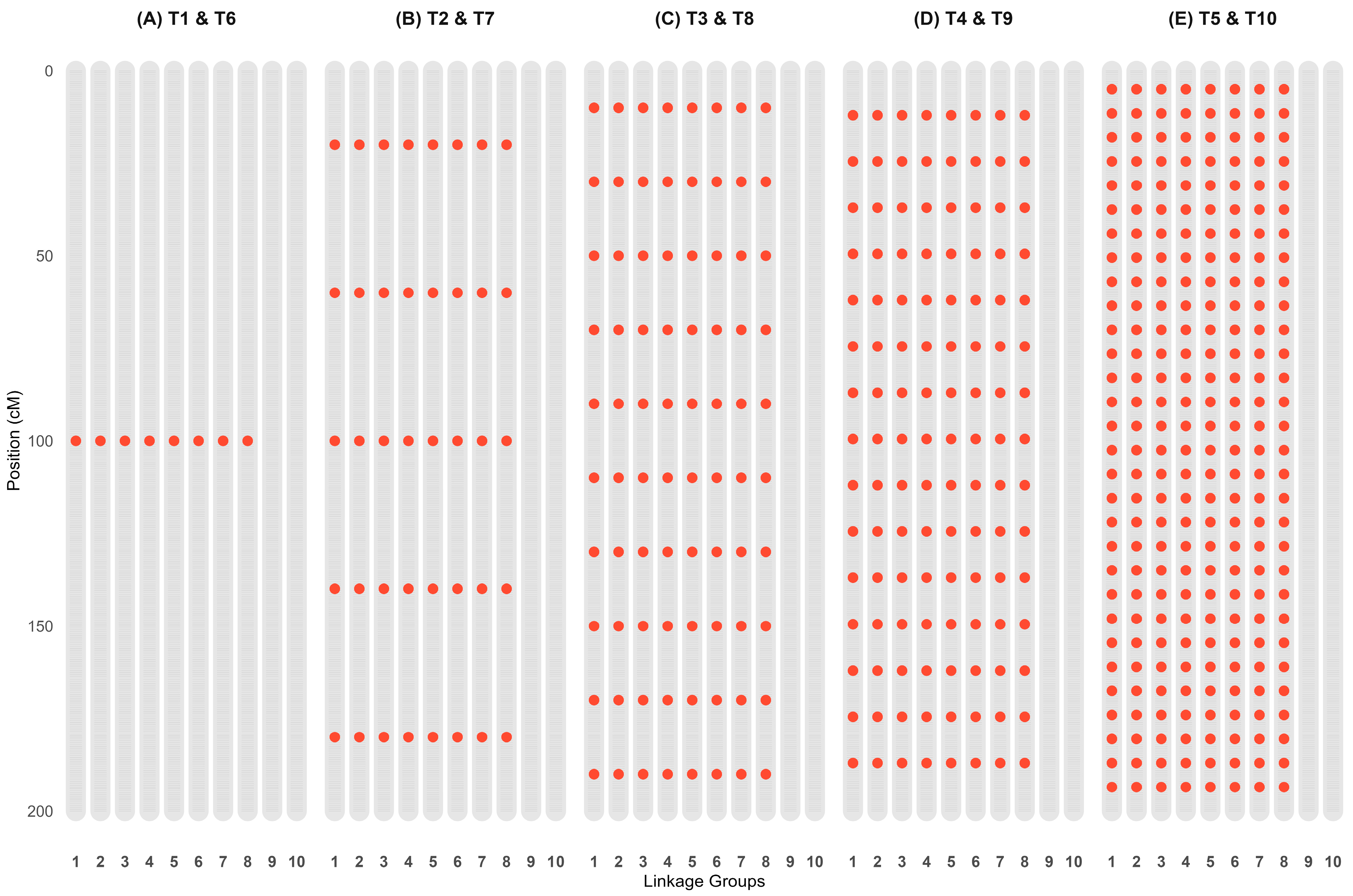
The controlling loci were equally distributed among the first eight LGs (Figure 1). Eight QTLs controlled traits T1 and T6 (Figure 1A), defined by the central markers of the first eight LGs (positions 201, 602, 1003, 1404, 1805, 2206, 2607, 3008, respectively). Whereas for traits T2 and T7 (Figure 1B), in addition to these central markers, other loci were incorporated by distributing QTLs equidistantly along these LGs. This design, although resulting in an overlap of some marker IDs, intentionally reflects contrasting genetic architectures between the trait sets. For traits T3 and T8 (Figure 1C), T4 and T9 (Figure 1D), and T5 and T10 (Figure 1E), QTLs were allocated across the first eight linkage groups with consistently spaced intervals between them, as illustrated in Figure 1. The distribution of QTLs was restricted to the first eight linkage groups. Linkage groups 9 and 10 were intentionally kept free of QTLs to serve as negative control regions (null chromosomes). This design was implemented to rigorously assess the Type I error rate (False Positives); any marker identified in these regions acts as a specific indicator of the method’s propensity to detect spurious associations in the absence of true genetic effect.

The total phenotypic values expressed by a given individual for the 10 traits were simulated, considering a mean of 100 and a coefficient of variation of 12%, with an average mean dominance degree of 0.5. An additive-epistatic model was adopted, and the phenotypic value ($Y_i$) of observation $i$ was modeled as follows [23]:

$$Y_i=\mu +\sum _j{\alpha }_j+\sum _j{\alpha }_j{\alpha }_{j+1}+e_i$$

(1)

where $\mu$ represents the population mean, and ${\alpha }_j$ denotes the additive effect of the favorable allele at locus $j$ for individual $i$. The genotypic values for homozygous dominant (AA), heterozygous (Aa), and homozygous recessive (aa) classes were assigned values of $u+a_i$, $u+d_i$ and $u-a_i$, respectively. Here, $u$ corresponds to the midpoint between the dominant (AA) and recessive (aa) homozygote means, with genotypic classes numerically coded as 1, 0, and −1. The term ${\alpha }_{ji}{\alpha }_{ji+1}$ quantifies epistatic interactions between alleles at distinct loci. Residual effects ($e$) followed a normal distribution $e~N\left(0,V_e\right)$, where residual variance $V_e$ was computed as $V_e=\left(\left(1-h^2\right)V_g\right)/h^2$, with $V_g$ denoting genotypic variance and $h^2$ the heritability.

2.2. Real Dataset

The genetic material comprised 195 Coffea arabica genotypes derived from crosses between the Catuaí group (susceptible) and the Timor Hybrid (HdT, resistant). The population included generations of Resistant Backcross ($B{C}_r$), Susceptible Backcross ($B{C}_s$), and $F_2$. The experiment was established in 2011 at the Experimental Station of the Federal University of Viçosa (Viçosa, MG, Brazil). Phenotypic evaluations were conducted in 2014, 2015, and 2016 for yield, measured as the volume of fresh coffee cherries (in liters) harvested per plant.

Genotyping of the 195 individuals was performed by RAPiD Genomics, Gainesville, FL, USA, using the Capture-Seq methodology. A set of 10,000 polymorphic probes, designed based on C. canephora genomic information and C. arabica EST sequences [24], was used, yielding 21,211 raw SNPs. To ensure data quality, rigorous filtering criteria were applied: Call Rate (CR) $\ge$ 90%, Minor Allele Frequency (MAF) $\ge$ 0.05, and the removal of SNPs with 100% observed heterozygosity, which indicate potential genotyping errors or paralogous sequences.

LD decay analysis was performed to define the genomic windows for QTL annotation. The squared correlation coefficient ($r^2$) between marker pairs was estimated using the LD.decay function from the sommer package [25]. A non-linear regression model was fitted to the data to determine the average distance at which $r^2$ decays to baseline thresholds. The analysis indicated that $r^2$ decayed to 0.8 at an average distance of 205 kb, which was subsequently used to define the QTL windows (Supplementary Figure S1).

For functional validation and gene annotation, the Coffea canephora reference genome [26] was used as a baseline, given its annotation quality and phylogenetic proximity as an ancestral subgenome of C. arabica. The gene annotation file (.gff3) was retrieved from the Coffee Genome Hub https://coffee-genome.org (accessed on 11 December 2025).

Gene mining was performed in the R environment using the Bioconductor suite, specifically the GenomicFeatures, rtracklayer, and GenomicRanges packages [27]. For each consensus genomic region identified by Machine Learning models, a search interval was defined based on the population’s estimated LD decay ($\pm$205 kb around the lead marker or spanning the clustered region). The coordinates of these regions were overlapped with annotated gene models to catalog all genes and their respective putative functions (gene products) located within the intervals of interest.

2.3. Formation of Regions

To define the regions associated with QTLs, a linkage disequilibrium (LD) analysis was conducted. Initially, the pattern of LD decay was assessed by plotting r² values as a function of genetic distance (in cM). Based on the average LD values among SNPs, the markers were grouped into non-overlapping genomic regions with specific sizes for each chromosome. Pairwise r² estimates for 4010 SNPs, derived from the squared correlation of allele frequencies, provided support for determining the appropriate length of each region.

The delimitation of the association window was performed by intersecting the curve fitted by LOESS with a horizontal line, thus defining which markers would be associated with a QTL. Therefore, markers located within the stipulated distance for the window, varying according to the evaluated scenario, were considered associated with the QTLs.

LD decay was quantified by computing the squared correlation coefficient (r²) via the LD.decay function within the sommer package [25]. The decay pattern was modeled using a nonlinear polynomial regression, and the resulting LD decay plot was generated using the R statistical software v. 4.5.1 to ensure reproducibility and visualization clarity.

2.4. Machine Learning (ML) Methods

All ML models were implemented in the R statistical environment. To ensure reproducibility, detailed mathematical formulations for the standard tree-based algorithms (Decision Trees—DT; Bagging—BA; Random Forest—RF; Boosting—BO) are in Supplementary Methods S1, while the specific implementation details and hyperparameters are described below.

2.4.1. Multivariate Adaptive Regression Splines (MARS)

The MARS algorithm [18] employs piecewise linear splines, termed basis functions (BFs), defined as

$${\left(x-t\right)}_{+}=\left\{\begin{array}{c}x-t,ifx>t,\\ 0,otherwise.\end{array}\right.$$

(2)

$${\left(t-x\right)}_{+}=\left\{\begin{array}{c}t-x,ifx<t,\\ 0,otherwise.\end{array}\right.$$

(3)

Each BF incorporates a knot at value t, with pairs of these functions (termed reflexive pairs) generated for each input marker $X_j$, using knots at observed values $X_{ij}$. The model construction follows a forward stepwise approach, iteratively selecting BFs or their interactions from the set $C={{\left(X_j-t\right)}_{+},{\left(t-X_j\right)}_{+}}_{t\in x_{1j},x_{2j},\dots ,x_{Nj}j=\mathrm{1,2},\dots ,p}$ to minimize residual error. The MARS model, a linear combination of BFs, is expressed as follows [28]:

$$f\left(X\right)={\beta }_0+\sum _{m=1}^M{\beta }_m{h}_m\left(X\right)$$

(4)

where ${\beta }_0$ is the intercept, ${\beta }_m$ are coefficients, and $h_m\left(X\right)$ represents BFs or their products.

The forward phase begins with $h_0\left(X\right)=1$, the algorithm adds the BF pair that maximally reduces training error. For a model with M terms, the added pair is [28]

$${\widehat{\beta }}_{M+1}{h}_l\left(X\right){\left(X_j-t\right)}_{+}+{\widehat{\beta }}_{M+2}{h}_l\left(X\right){\left(t-X_j\right)}_{+},h_l\in M$$

(5)

where ${\widehat{\beta }}_{M+1}$ and ${\widehat{\beta }}_{M+2}$ are estimated via least squares. This continues until a predefined maximum (e.g., 200 terms), often resulting in overfitting [29].

In the backward, insignificant terms are pruned using Generalized Cross-Validation (GCV), which balances fit and complexity [26]:

$$GCV\left(\lambda \right)={\displaystyle \frac{\frac{1}{N}{\sum }_{i=1}^N{\left[y_i-{\widehat{f}}_{\lambda }\left(x_i\right)\right]}^2}{{\left[1-\frac{C\left(M\right)}{N}\right]}^2}}$$

(6)

where $C\left(M\right)=3$ (default) penalizes model complexity [18], N is the sample size, and ${\widehat{f}}_{\lambda }\left(x_i\right)$ denotes the predictions.

Models were trained using three distinct configurations of interaction degrees: 1 (additive effects only), 2 (pairwise interactions), and 3 (three-way interactions). The forward phase was terminated when the maximum number of terms was reached (default limit of 200) or if the improvement in the model’s goodness-of-fit fell below the default forward stepping threshold (‘thresh = 0.001’). This parameter was maintained at the default value to prioritize model convergence across high-dimensional genomic datasets, ensuring that the final model selection relied primarily on the GCV criterion during the backward pruning phase.

2.4.2. Decision Tree (DT)

The DT architecture was constructed by iteratively partitioning the dataset into maximally homogeneous subgroups using recursive binary splitting. The selection criterion prioritizes splits that achieve the maximal reduction in the Residual Sum of Squares (RSS). To balance model complexity and interpretability, the maximum depth was set to 30, and the minimum leaf size was set to 6 (calculated as the rounded minimum number of observations required for a split divided by 3).

2.4.3. Bagging (BA)

The BA algorithm [30,31] enhances the stability of regression trees by generating multiple bootstrapped datasets through resampling. For each dataset, an unpruned regression tree is trained, and the final ensemble prediction is derived by averaging the outputs of all trees. In this study, the algorithm was configured with 500 decision trees to ensure robust estimation stability.

2.4.4. Random Forest (RF)

RF [32] extends the bagging approach by introducing stochasticity at the node level. While it also utilizes bootstrapped datasets to construct an ensemble, RF restricts each split to a randomly selected subset of predictors ($m\approx p/3$, where $p=4010$ markers). This decorrelates the trees and mitigates overfitting. We utilized an ensemble size of 500 trees, a parameter empirically validated for stability in high-dimensional genomic contexts.

2.4.5. Boosting (BO)

The BO algorithm iteratively constructs an ensemble where each new tree focuses on correcting the residuals (errors) of the previous iterations [33]. Unlike parallel methods (BA/RF), BO operates sequentially within a gradient-based optimization framework. Key hyperparameters included 500 trees, a learning rate (shrinkage) of 0.01, and an interaction depth of 2 to restrict model complexity. Default regularization settings were maintained (bag fraction = 0.5, minimum observations in node = 10) to prevent overfitting.

2.5. Genome-Wide Association Study (GWAS) Models

To establish a robust baseline for comparison against ML methods, we employed a comprehensive suite of GWAS algorithms implemented in the GAPIT package (v3.5.0) [34]. Instead of relying on a single model, we evaluated seven distinct statistical frameworks, ranging from traditional single-locus models to state-of-the-art multi-locus methods:

GLM (General Linear Model): A naive baseline fitting markers as fixed effects with Principal Component Analysis (PCA) as covariates to account for population structure.

MLM (Mixed Linear Model): Incorporates both PCA (fixed effects) and a Kinship matrix (random effects) to control for cryptic relatedness and population stratification [35].

CMLM (Compressed Mixed Linear Model): Groups individuals into clusters to reduce the effective sample size of the random effect, improving statistical power [35].

MLMM (Multi-Locus Mixed Model): Uses a stepwise forward–backward regression approach to include significant markers as covariates [36].

SUPER (Settlement of MLM Under Progressively Exclusive Relationship): A method that increases statistical power by extracting a subset of pseudo-QTNs to use as covariates in a mixed model framework, effectively separating true genetic signals from confounding population structure [37].

FarmCPU (Fixed and random model Circulating Probability Unification): An iterative method that alternates between a fixed-effect model (testing markers) and a random-effect model (using significant markers to define kinship), effectively controlling false positives while maintaining high power [38].

BLINK (Bayesian-information and Linkage-disequilibrium Iteratively Nested Key): An evolution of FarmCPU that eliminates the requirement for the computationally expensive kinship matrix, replacing it with a Bayesian Information Criterion (BIC) and LD-based pruning to select covariates. It is currently considered one of the state-of-the-art methods for large datasets [39].

For all models, population structure was corrected using the first three Principal Components (PCs) derived from the genomic relatedness matrix. The significance threshold for marker-trait associations was determined using the Bonferroni correction ($\alpha =0.05$).

2.6. Statistical Evaluation and Performance Metrics

2.6.1. Cross-Validation Scheme

To ensure the statistical robustness of the results and mitigate sampling bias, a rigorous nested cross-validation scheme was implemented. The experimental design consisted of 10 independent replicates, each subjected to a 5-fold cross-validation, totaling 50 independent evaluation cycles per genetic scenario.

To guarantee a fair comparison, we employed a paired experimental design: for every fold, the datasets were pre-partitioned into fixed training (80%, $n=800$) and validation (20%, $n=200$) sets. These identical file sets were fed into all ML methods (MARS, DT, BA, RF, BO) and the multi-locus GWAS pipeline (GLM, MLM, CMLM, MLMM, SUPER, FarmCPU, BLINK). This approach eliminates sampling variance between methods, ensuring that performance differences are solely due to algorithmic capability [40]. Additionally, a random seed, set.seed (123), was enforced within the computational scripts to ensure the exact reproducibility of stochastic learning processes.

2.6.2. Marker Importance and Selection Thresholds

Marker importance for MARS was determined by quantifying the reduction in RSS across all subsets where a marker is present. The algorithm sums these cumulative RSS reductions, with larger reductions indicating greater marker importance [41]. This quantification was performed using the varImp function from the caret package in the R software. In summary, MARS establishes its optimal model structure through an iterative two-step process: it first employs forward selection to add candidate basis functions that capture non-linear relationships and interactions, and then applies backward pruning, guided by GVC, to eliminate redundant terms.

In DT, variable importance is assessed by the frequency with which each variable is used to split the tree’s nodes, weighted by the improvement in accuracy that each split provides. In RF, BA, BO the importance was calculated by averaging the decrease in the RSS. The varImp function from the caret package of the R software was used. These methods evaluate variable importance by looking at how often and effectively a variable contributes to reducing prediction errors. In DT, this is through the weighted frequency of splits, while in ensemble methods like RF, BA, BO, it is quantified by the average reduction in residual errors.

To ensure comparability across algorithms, all importance scores were normalized to a common scale ranging from 0 to 10. To classify a marker as associated or not associated in ML models, we applied a dynamic empirical threshold on these normalized scores: markers with an importance score above the mean importance of that replicate were considered selected. This data-driven approach allows for fair comparisons across methods with different importance scales.

For the GWAS modeling the individual marker, effects on phenotype values were estimated, and statistical significance was determined through multiple hypothesis testing. Bonferroni-corrected ${-log}_{10}\left(P\right)$ thresholds identified significant SNPs at 5%.

To ensure the robustness of the findings in the real data analysis, a consensus calling criterion was established. A genomic region was classified as a high-confidence candidate only if it was independently identified by at least two distinct model configurations (e.g., different ML algorithms).

2.6.3. Performance Metrics

The performance of each method was evaluated by calculating the Mean and Standard Deviation (SD) of the metrics across the 50 independent runs. The SD served as the primary proxy for algorithmic stability. Methods with lower SD values were considered more robust to variations in the training data partition and stochastic initialization, regardless of slight fluctuations in mean values.

• Detection Power (DP): Represents the proportion of windows or regions, previously defined through LD analysis, that contain at least one marker identified as significant. This metric evaluates the method’s effectiveness in detecting true signals within the regions of interest.
• False Positive Rate (FPR): Quantifies the proportion of non-associated SNPs incorrectly flagged as significant, defined as the fraction of markers falsely linked to the trait relative to the total non-causal SNPs. This metric reflects the statistical noise in association mapping.
• Precision: Evaluates the method’s specificity in detecting true QTLs. High precision indicates robust discrimination between true associations and genomic background noise, critical for prioritizing candidate loci in downstream analyses.
• Specificity: Evaluates the method’s ability to correctly recognize markers that are not associated with the trait, that is, the true negatives. High specificity indicates that the method avoids incorrectly classifying markers without effect associated.

2.7. Computational Resources

Population genetic simulations were implemented in the Genes software [22]. DT, RF, BA, BO, and MARS were executed within the R computational environment. For GWAS model parameterization, marker effect coefficients were estimated through ordinary least squares (OLS) regression, minimizing the residual sum of squares using the GAPIT package in R [34].

All statistical and ML analyses were performed on a Windows 11 Home Single Language (×64) platform, utilizing a notebook equipped with an Intel^® Core™ Ultra 7 155H processor (3.80 GHz), Intel Corporation, Mountain View, CA, USA, and 32 GB of RAM. To optimize performance, the computationally intensive tasks, specifically the cross-validation folds for ML and the multi-model GWAS scans, were executed using parallel processing implemented via the doParallel and foreach packages in R. The reproducibility of the analysis is ensured by the use of specific R package versions, including earth (v5.3.4) for MARS, randomForest (v4.7–1.2), gbm (v2.2.2), and GAPIT (v3.5.0). A complete list of all package versions and detailed hyperparameter settings is provided in Supplementary Table S1.

3. Results

3.1. Simulated Data Analysis

3.1.1. Linkage Disequilibrium

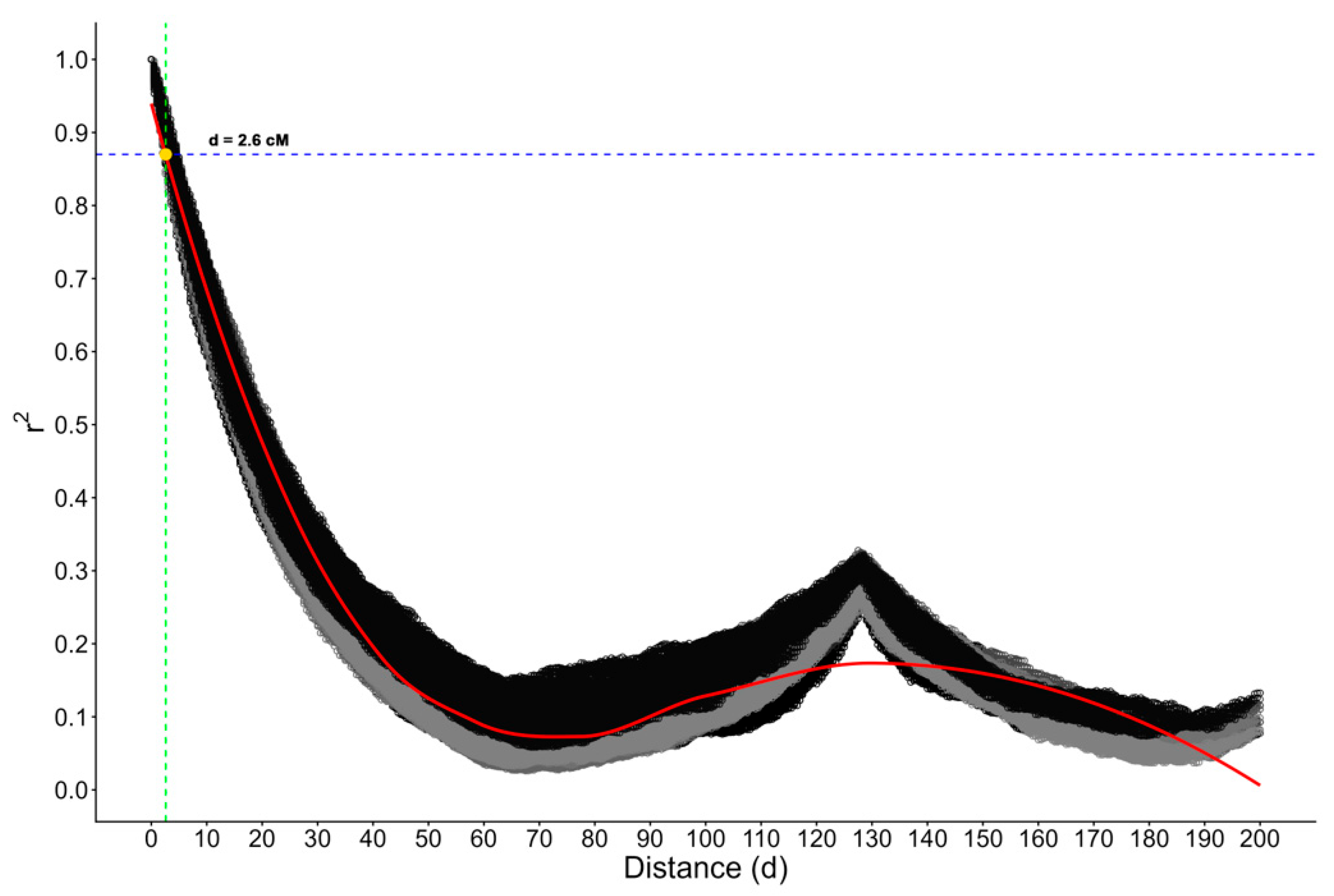
Due to the high marker saturation (4010 markers every 0.50 cM in each GL of 200 cM), an LD value of 0.87 was considered as the threshold for determining the size of the regions. This value corresponds to a genetic distance (d) of 2.6 cM (Figure 2), as also adopted by [42]. Thus, the region considered as the QTL would be represented by the five markers before and after the QTL, encompassing a window of approximately 5 cM and covering eleven markers, with the central marker corresponding exactly to the QTL of interest.

3.1.2. Detection Power (DP)

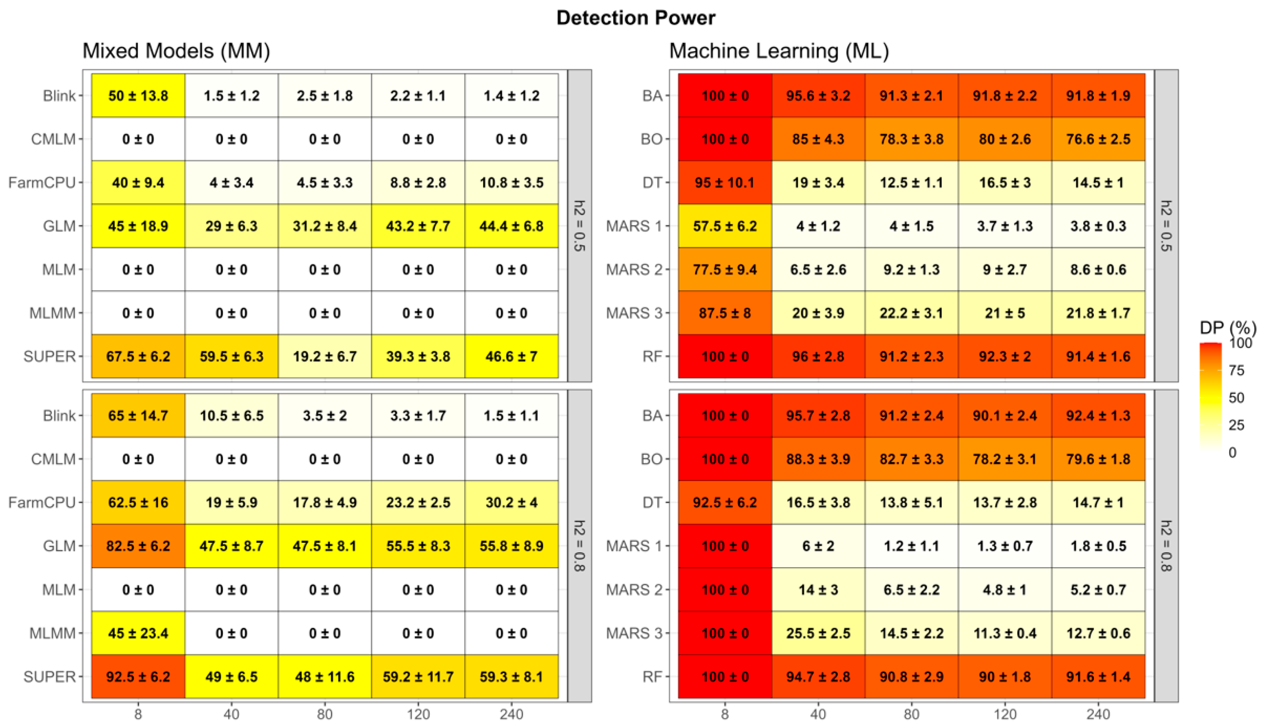
The sensitivity of the methods was evaluated via DP across genetic architectures ranging from oligogenic (8 QTLs) to highly polygenic (240 QTLs). The analysis revealed a stark contrast between ML ensembles and statistical LMMs (Figure 3).

Ensemble methods demonstrated remarkable stability and superior sensitivity. In oligogenic traits ($n_{genes}=8$), BA, BO, and RF consistently achieved 100% DP, effectively capturing all simulated causal variants regardless of heritability. Notably, this robustness persisted in high-complexity scenarios. For instance, in the most polygenic scenario evaluated (240 genes, $h^2=0.8$), BA and RF maintained mean DP values of 92.4% (±1.3) and 91.6% (±1.4), respectively. This confirms that tree-based ensembles are highly effective at minimizing false negatives, successfully recovering the vast majority of genetic signals even in the presence of extensive epistasis.

In contrast, traditional statistical frameworks exhibited severe limitations in these epistatic scenarios. Standard MLM and CMLM suffered a complete collapse in sensitivity, yielding 0% DP across almost all scenarios (e.g., traits with 8 to 120 genes under moderate heritability $h^2=0.5$). This highlights that the standard interaction of polygenic background correction with stringent Bonferroni thresholds renders these methods overly conservative for the specific genetic architectures simulated here.

However, among the multi-locus methods, SUPER demonstrated exceptional performance, establishing itself as the most sensitive GWAS algorithm. In oligogenic scenarios characterized by high heritability ($n_{genes}=8$, $h^2=0.8$), SUPER achieved a Detection Power (DP) of 92.5% (±6.2), outperforming the naive GLM (82.5%) and significantly surpassing BLINK (65.0%) and FarmCPU (62.5%). Furthermore, as complexity increased to polygenic architectures (240 genes, $h^2=0.8$), SUPER maintained a robust DP of 59.3% (±8.1). This represents a substantial improvement over FarmCPU, which dropped to 30.2% (±4.0), and BLINK, which captured only 1.5% (±1.1) of the signals.

While SUPER significantly narrowed the gap between statistical methods and Machine Learning, a “sensitivity gap” remains. In the most complex scenario (240 genes, $h^2=0.8$), the best ML method (BA) still detected considerably more QTLs than the best GWAS method (SUPER) (~92% vs. 59.3%). This confirms that while SUPER is highly effective compared to its statistical peers, Ensemble methods provide the maximal recovery of missing heritability in complex epistatic traits.

The GLM showed high sensitivity (e.g., 82.5% in the 8-gene, $h^2=0.8$ scenario and 55.8% in the 240-gene, $h^2=0.8$ scenario), often surpassing advanced models. However, as discussed in the subsequent sections, this high detection power is typically inflated by the lack of kinship correction, leading to a higher rate of spurious associations.

3.1.3. Precision

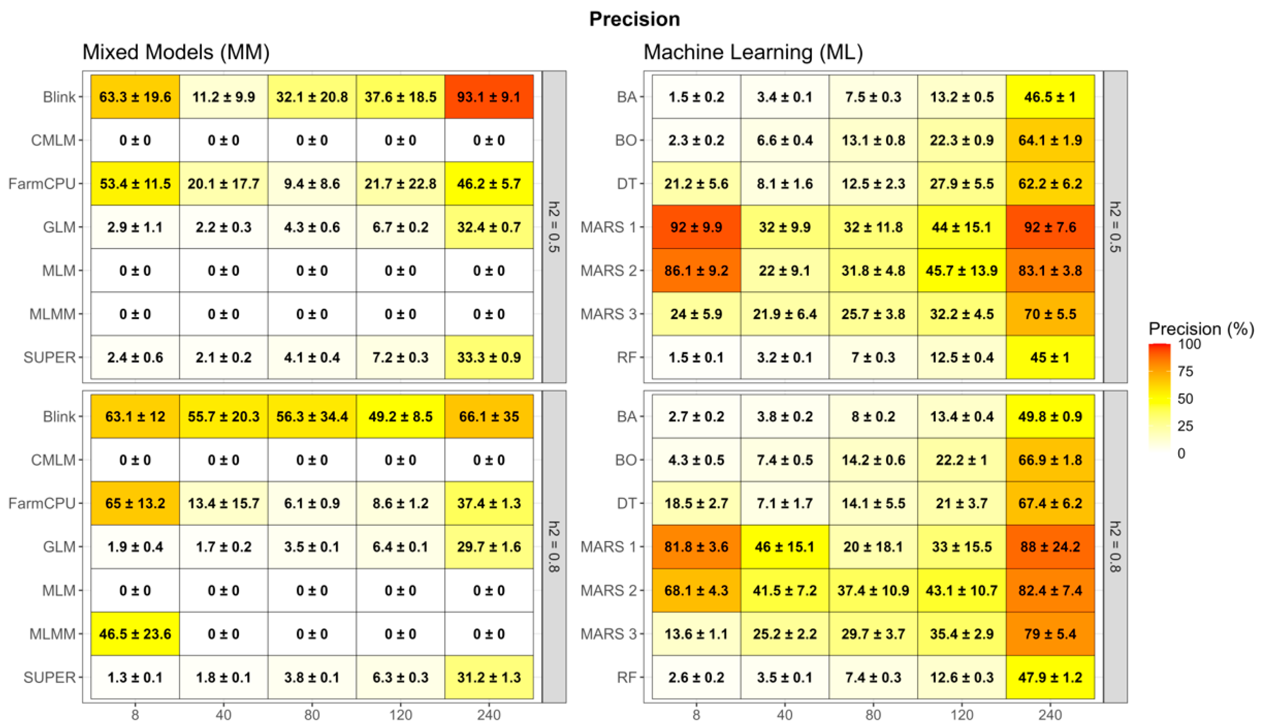
Precision consistently improved as the number of QTLs increased, revealing a fundamental dynamic in marker prioritization: as the density of true causal variants rises within the genome, the probability of a selected marker being a True Positive increases. While ensemble methods excelled in broad detection, the analysis of Precision highlighted the inherent trade-off between sensitivity and signal reliability (Figure 4).

In scenarios characterized by simple genetic architectures ($n_{genes}=8$), tree-based ensembles (BA, RF) exhibited low precision. For instance, in the moderate heritability scenario ($h^2=0.5$), BA achieved a precision of only 1.5% (±0.2). This is a direct mathematical consequence of their broad capture strategy: to achieve 100% detection power, these algorithms selected a large number of correlated markers, thereby diluting the proportion of true positives. However, in highly polygenic scenarios (240 genes, $h^2=0.8$), their precision improved significantly to 49.8% (±0.9) for BA, confirming their utility for genomic screening in complex traits where the signal density is higher.

In stark contrast, MARS-based methods (specifically Degree 1) acted as highly conservative filters. Although MARS 1 presented lower sensitivity in complex traits compared to RF, its precision was exceptional. In the moderate heritability polygenic scenario (240 genes, $h^2=0.5$), MARS 1 achieved a precision of 92.0% (±7.6). This indicates that when the additive MARS algorithm identifies a marker, there is a very high probability that it is a true causal variant. Notably, increasing the model complexity to Degree 3 (MARS 3) reduced precision (dropping to 70.0% in the same scenario), suggesting that modeling higher-order interactions without strict regularization introduces significant false positive noise compared to the additive baseline.

Among the GWAS frameworks, the comparison between SUPER and BLINK reveals a critical methodological divergence. While SUPER dominated in detection power (Section 3.2), this came at a severe cost to precision. In the high-heritability oligogenic scenario (8 genes, $h^2=0.8$), SUPER achieved a precision of only 1.3% (±0.1), comparable to the naive GLM (1.9%). This suggests that SUPER achieves high sensitivity by relaxing the filtering of population structure, resulting in a “noisy” selection similar to fixed-effect models.

Conversely, BLINK emerged as the undisputed leader in statistical precision. In the highly polygenic scenario (240 genes, $h^2=0.5$), BLINK achieved a precision of 93.1% (±9.1), drastically outperforming both FarmCPU (46.2% ± 5.7) and SUPER (33.3% ± 0.9). Even in the high heritability scenario ($h^2=0.8$) where noise is amplified, BLINK maintained 66.1% precision while SUPER dropped to 31.2%. This positions BLINK (alongside MARS 1) as the ideal tool for candidate gene validation, offering superior specificity, whereas SUPER serves better as a broad screening tool similar to Ensembles.

3.1.4. False Positive Rate (FPR) and Specificity

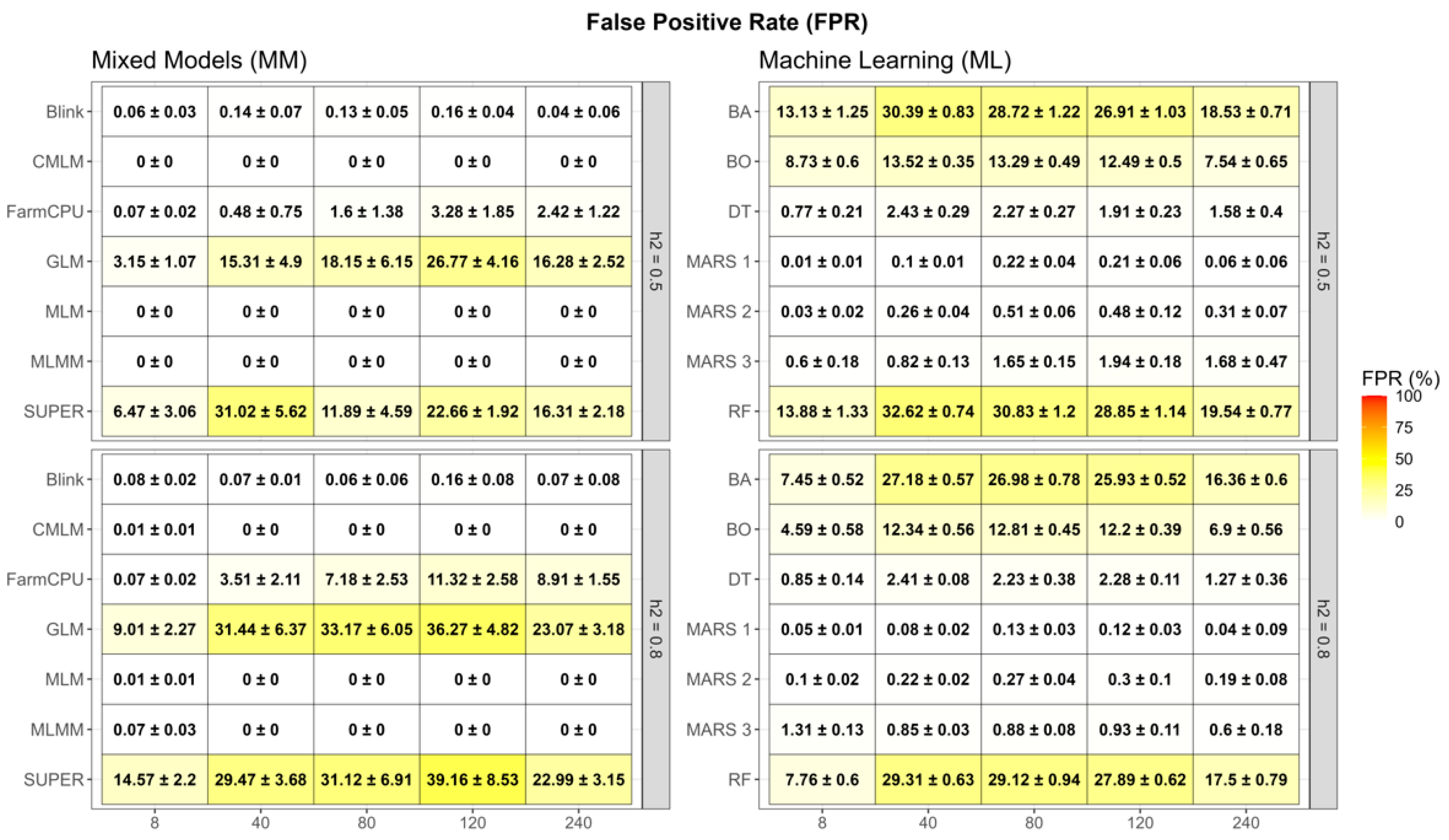
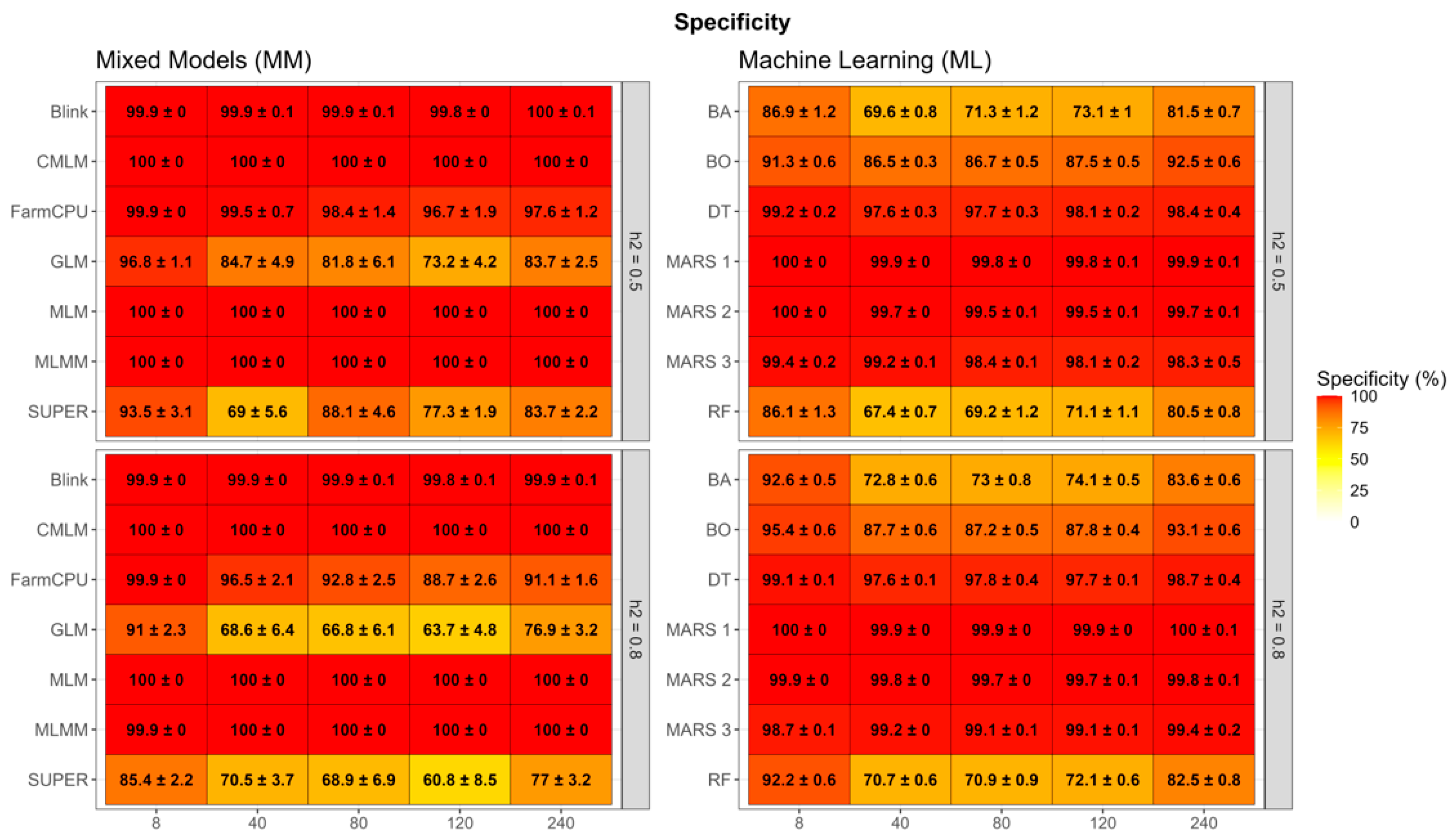
The assessment of Type I error control, measured via FPR and Specificity, revealed critical distinctions between methodologies (Figure 5 and Figure 6). While ensemble methods excelled in detection power, this sensitivity incurred a substantial cost in terms of signal purity compared to regression-based strategies.

A clear trade-off was observed within the ML category. Tree-based ensembles (BA, RF), which utilized a mean importance threshold, exhibited the lowest specificity across all evaluated scenarios. In scenarios with moderate complexity (e.g., 40 genes, $h^2=0.5$), RF achieved a specificity of only 67.4% (±0.7), corresponding to a high FPR of ~32.6%. BA followed a similar trend (69.6% ± 0.8). This confirms that these methods capture a wide genomic context, including markers in weak LD with causal variants, rather than pinpointing the exact QTNs. BO proved to be more efficient, maintaining higher specificity (e.g., 86.5% in the same scenario) due to its sequential learning process.

In stark contrast, MARS-based algorithms (specifically Degree 1) demonstrated near-perfect specificity, functioning as highly robust filters against noise. Even in highly polygenic traits (240 QTLs, $h^2=0.8$), MARS 1 achieved a specificity of 100% (±0.1), effectively reducing the FPR to negligible levels (0.04%). This explains its superior Precision (Section 3.1.3) but also accounts for its lower DP, as the algorithm aggressively prunes potential signals to satisfy the GCV criterion.

Among statistical models, the analysis revealed a distinct spectrum of error control. Standard mixed models (MLM, CMLM, MLMM) achieved 100% Specificity across virtually all scenarios, but as noted in Section 3.1.2, this came at the cost of zero detection power.

The advanced multi-locus methods diverged into two distinct performance profiles regarding error control. BLINK paralleled the ultra-high specificity of MARS 1, maintaining values exceeding 99.8% even in the most complex scenarios. It consistently minimized the False Positive Rate (FPR), limiting it to just 0.04% in the 240-gene, $h^2=0.5$ scenario, thereby proving to be the most robust statistical filter among the evaluated frameworks. Conversely, SUPER, consistent with its prioritized detection power, exhibited significantly higher error rates. In high-complexity scenarios (120 genes, $h^2=0.8$), the specificity of SUPER dropped to 60.8% (±8.5), corresponding to an FPR of 39.1%. This performance mirrors the “noisy” profile of the naive GLM (Specificity ~63.7% in the same scenario), indicating that SUPER’s algorithmic strategy of selecting pseudo-QTNs, while effective for signal capture, simultaneously admits a substantial amount of background noise.

FarmCPU occupied a middle ground, maintaining good specificity (>88%) in most cases, but showing signs of inflation (FPR ~11.3%) in high-heritability complex traits. Thus, for applications prioritizing “clean” results, BLINK and MARS 1 are the optimal choices, while SUPER behaves more like an Ensemble method, prioritizing discovery over purity.

3.1.5. Computational Efficiency Analysis

In addition to detection accuracy, we evaluated the computational efficiency of each method (

Table 3. Computational efficiency of GWAS and Machine Learning methods. Values represent the mean processing time ($\pm$standard deviation) per replicate required to analyze a single trait with 4010 markers and 1000 individuals.

Method Category	Algorithm	Mean Time (s)	Minimum Time (s)	Maximum Time (s)
Mixed Models	BLINK	67.95 ± 13.64 s	41.28	155.18
	FarmCPU	83.17 ± 13.89 s	60.55	125.15
	SUPER	2185.82 ± 4194.49 s	230.15	18,071.06
	GLM	98.42 ± 16.34 s	49.48	140.37
	MLM	165.11 ± 19.97 s	141.23	205.31
	MLMM	318.53 ± 38.65 s	269.61	426.73
	CMLM	710.71 ± 70.33 s	610.82	837.20
Machine Learning	DT	12.6 ± 1.8 s	6.24	16.58
	MARS 1	32.36 ± 2.59 s	25.76	42.99
	MARS 2	81.66 ± 20.32 s	47.73	136.08
	MARS 3	400.67 ± 130.23 s	160.14	692.06
	BA	663.24 ± 61.22 s	384.35	762.91
	BO	50.4 ± 5.11 s	27.29	61.49
	RF	243.04 ± 22.76 s	145.84	290.64

). The LMMs demonstrated heterogeneous performance: state-of-the-art multi-locus methods were highly efficient, with BLINK and FarmCPU requiring on average 67.9 s and 83.2 s per replicate, respectively. However, the SUPER algorithm proved to be computationally prohibitive and highly unstable. It required an average of 2185.8 s per replicate, with extreme variability (SD ± 4194.5 s) and peak times exceeding 5 h (18,071 s), identifying it as the most resource-intensive method overall. Traditional iterative approaches like CMLM were also demanding (710.7 s), surpassing most ML models.

Among ML approaches, DT was the fastest algorithm overall (12.6 s), followed by MARS 1 (32.4 s) and BO (50.4 s), which proved to be surprisingly competitive with fast GWAS methods. In contrast, ensemble methods reliant on bagging mechanisms exhibited higher costs: RF averaged 243.0 s, and BA required 663.2 s.

In summary, a critical trade-off emerges. Adopting a robust ensemble strategy like BA entails a ~10-fold increase in time compared to fast methods like BLINK. However, BA is approximately 3× faster than the SUPER model, while providing significantly higher detection power. This suggests that for complex traits, Machine Learning ensembles offer a more favorable balance between computational cost and discovery potential than complex parameterized GWAS models.

3.2. Real Data Analysis

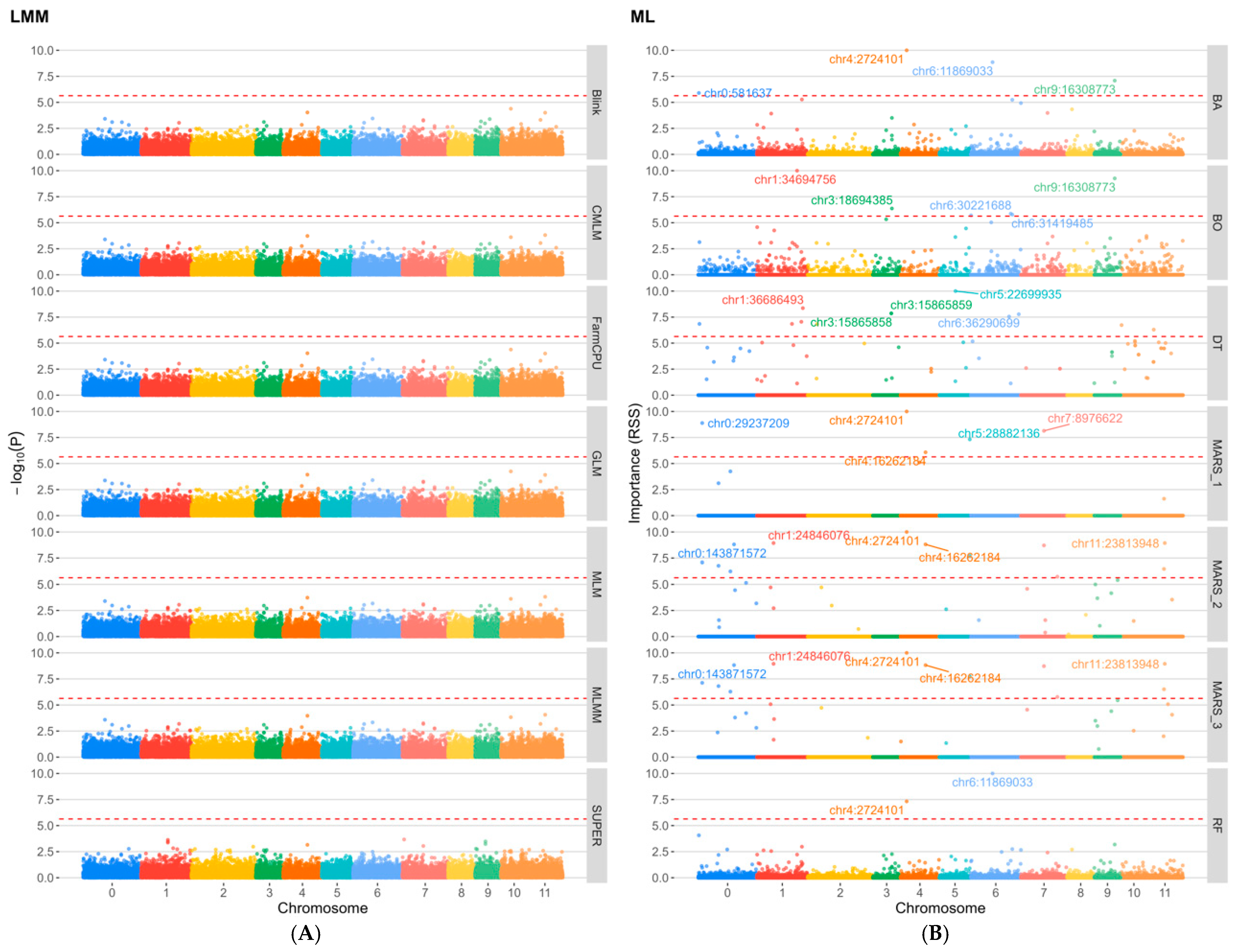
While the standard GWAS models failed to detect significant associations after Bonferroni correction ($\mathrm{\alpha }=0.05$), likely due to the highly polygenic architecture of coffee yield and the strict penalty on false positives, the ML framework successfully prioritized 53 SNP markers with importance scores exceeding the significance threshold (Figure 7).

Among the ML-selected markers, SNP chr4:2724101 (Chromosome 4) emerged as the most robust candidate, being independently identified by five different algorithms. Other highly recurrent markers included chr0:29237209 (unanchored scaffold), chr4:16262184, chr5:28882136, and chr7:8976622, each detected by three distinct models. Regarding model performance, non-parametric methods such as DT and MARS (degree 2 and 3) demonstrated higher sensitivity, selecting 12 markers each, whereas RF was the most conservative, selecting only 2 markers (Figure 7).

To facilitate biological interpretation, the 53 significant SNPs were grouped into genomic regions based on the previously determined LD decay window of 205 kb. This resulted in 30 distinct regions associated with yield (Table S2). Notably, regions Chr11_R2 (Chr 11: 23.63–23.81 Mb) and Chr3_R1 (Chr 3: 15.86 Mb) were highlighted as high-confidence QTLs, containing multiple significant hits clustered within the linkage block (Table S2). To provide a clearer biological context for the peaks observed in Figure 7, we summarized the highest-confidence findings in Supplementary Table S3. This table details the top 5 genomic regions identified by the consensus of machine learning models, highlighting key candidate genes and their functional categories, such as stress response regulators and metabolic enzymes, which are relevant for coffee breeding.

4. Discussion

The accuracy of QTL detection via LD between marker loci and causal variants is contingent upon both the magnitude of LD and its decay rate across the genomic interval separating markers and causal loci within a population [43]. To achieve a single-gene level resolution in determining the association between a marker and the phenotype, the linkage block size must be extremely reduced. Consequently, the minimal genomic interval yielding the predefined LD threshold can delineate chromosomal LG regions, thereby establishing the critical LD threshold for downstream statistical analyses [44].

In an F₂ population, where LD arises solely from factorial linkage [23], the genetic correlation between loci is determined by recombination frequency (r). Thus, loci separated by 2.5 cM have a recombination rate of 0.025 (2.5%). In this case, considering r = 0.025, the genetic correlation given by [44]: $r^2=\sqrt{\left(1-2r\right)}$ will be approximately 0.98, indicating that close markers are strongly associated with the QTL due to the high level of LD resulting from genetic proximity. This demonstrates that an LD value of 0.87 corresponds to a strong association between the marker and the QTL present in the defined 5 cM window, with the central marker corresponding to the simulated QTL. Previous studies [42] adopted association windows of different sizes, ranging from 1 to 5 cM. Analysis of the simulated traits revealed epistatic interactions, as evidenced by a secondary elevation in LD (r²) between markers spaced ~130 cM apart within the same LG. This bimodal LD pattern underscores the contribution of non-additive genetic architecture to trait variation.

4.1. Performance of ML Methods in Complex Scenarios

Our results demonstrate a clear dichotomy in method performance driven by the complexity of the genetic architecture. While traditional LMM-based GWAS proved adequate for simple traits, their performance degraded severely as genetic complexity increased. The substantial advantage of ML methods in these high-complexity scenarios (e.g., 240 QTLs) can be attributed to their fundamental algorithmic structures, which differ radically from the linear additivity assumed by mixed models.

The specific advantage of MARS lies in its non-parametric approach using hinge functions (basis functions) and knot optimization. By explicitly modeling interactions as products of these basis functions (e.g., $max\left(0,x-t\right)\times max\left(0,z-k\right)$), MARS can map the non-linear response surfaces generated by epistasis without requiring the user to specify interaction terms a priori [18]. This adaptive approach allows MARS to automatically detect and model higher-order interactions, which are crucial for identifying epistatic effects [13]. Similarly, BO constructs an ensemble of weak learners that sequentially focus on difficult-to-predict instances (residuals), effectively learning the complex genetic architecture that linear models treat as noise.

Ensemble learning methods (BA, RF) demonstrated robust DP, reaching 100% in oligogenic scenarios and maintaining levels above 90% even in highly polygenic traits (240 genes, $h^2=0.8$). This significantly outperformed state-of-the-art GWAS methods like FarmCPU, which plateaued at approximately 30.6% sensitivity in the same complex scenarios. While the SUPER algorithm bridged the sensitivity gap (reaching ~60% DP), it mirrored the behavior of the naive GLM by inflating False Positive Rates (~39%), confirming that its strategy of selecting pseudo-QTNs captures true signals but fails to filter background noise effectively. The divergent performance of the SUPER algorithm, displaying relatively high Detection Power but lower Precision, can be attributed to its methodological design. SUPER employs a pre-selection strategy using a FaST-LMM approach to retain a subset of ‘pseudo-QTNs’ as covariates [37]. While this aggressive inclusion enhances sensitivity by effectively reducing residual variance, in complex epistatic scenarios, it appears to increase the risk of overfitting. This often leads to the retention of false positives or markers that are merely in linkage disequilibrium with the true signals, unlike BLINK, which employs a stricter exclusion criterion.

Regarding computational efficiency, it is noteworthy that the SUPER algorithm exhibited a remarkably high standard deviation in runtime (±4194 s). This extreme variability stems from the iterative nature of the aforementioned pseudo-QTN selection process. In simulation replicates with complex genetic architectures or high marker density, the optimization of the kinship matrix requires significantly more cycles to converge compared to simpler scenarios. This leads to occasional extreme runtimes, in sharp contrast to the stable computational costs demonstrated by ML ensembles and other GWAS models.

Consequently, sensitivity in Ensembles came at a cost in specificity. RF and BA exhibited FPR reaching ~30–32% in moderate complexity scenarios, confirming that these methods prioritize minimizing False Negatives by capturing a broad genomic context, often including markers in weak LD. This behavior aligns with findings in genomic prediction, where ensembles consistently outperform linear kernels by capturing global epistatic variance [45,46].

MARS Degree 1 (additive) functioned as a highly precise filter. While its detection power was lower in complex traits compared to Ensembles, its Precision was exceptional. In the polygenic scenario with moderate heritability (240 genes, $h^2=0.5$), MARS 1 achieved a precision of 92.0% and a specificity of 100%, effectively reducing the FPR to negligible levels (0.04%). This leverages the algorithm’s capacity to rigorously prune variables during the backward selection phase based on GCV [18]. Interestingly, increasing complexity to MARS 3 (Degree 3) improved detection power but reduced precision, illustrating how modeling higher-order interactions introduces noise if not strictly regularized.

The enhanced detection power of ML methods relative to conventional GWAS is significant for the missing heritability problem. While the naive GLM and SUPER showed high detection power, they suffered from inflated FPR comparable to noisy ensembles. Advanced methods like BLINK and FarmCPU excelled at controlling FPR (Specificity > 99%), matching the clean profile of MARS 1. However, they missed a substantial portion of the heritability in complex scenarios (DP ~30–34% vs. ML’s ~92%), rendering them overly conservative for traits where the primary goal is to uncover the complete genetic architecture. This behavior is typical of linear models in data with high multicollinearity, where spurious effects are inflated [47]. Several studies have further highlighted that GLM and MLM-based methods tend to produce high FP rates [48,49], with some reports indicating FPR exceeding 40% [50], a limitation confirmed here by the performance of SUPER and GLM and frequently reported when linear models face high multicollinearity and cryptic population structure [50,51].

Methods such as MARS 1 and BLINK are therefore recommended for scenarios requiring high specificity (candidate gene validation), while Ensemble methods are ideal for maximizing signal recovery. As reported in [47], there is no golden rule for variable selection; the model selection must be aligned with the breeding objective, whether it be precise gene identification or comprehensive genomic prediction.

4.2. Practical Implications: A Decision Framework

When selecting a GWAS method, researchers must navigate the trade-off between computational cost, detection sensitivity, and signal precision. Based on our findings, we propose a decision framework where the choice is guided by the complexity of the phenotype and the specific goals of the breeding program.

For traits hypothesized to be governed by major genes with additive effects, such as qualitative resistance to pathogens, and where heritability is high, standard LMM-based GWAS or fast multi-locus methods like BLINK remain the preferred choice. These models offer significantly lower computational costs, direct interpretability of p-values, and rely on established software ecosystems [52]. Since our simulations demonstrated that advanced GWAS methods perform comparably to ML in simple architectures, the additional computational effort required by complex algorithms is unnecessary in these specific scenarios.

In contrast, for quantitative traits where epistasis is suspected, such as yield or drought tolerance, or where standard GWAS fails to explain a significant portion of the genetic variance, Ensemble ML methods, specifically BA and RF, should be prioritized. The trade-off here is quantitative and justified: while these methods required approximately 10 times more computational time than optimized GWAS frameworks in our experimental setup (Section 3.1.5), they were approximately 3× faster than the SUPER model, the only statistical method that approached their sensitivity levels. In complex scenarios involving 240 QTLs, the detection power of FarmCPU dropped to approximately 30%, whereas BA and RF maintained power above 90%. This confirms that for exploratory screenings where minimizing False Negatives is the priority, Ensembles are the most viable option to recover missing heritability [53], offering a better balance of speed and power than complex parameterized LMMs.

Furthermore, the choice of algorithm must align with the specific stage of the breeding pipeline. Our results highlight a distinct role for MARS (Degree 1) compared to Ensembles. Unlike Bagging, which maximizes discovery at the cost of higher FPR, MARS 1 functions as a conservative filter, achieving precision and specificity (>99%) comparable to BLINK. Therefore, if the breeder’s goal is candidate gene validation, where false positives result in costly downstream errors, MARS 1 or BLINK are recommended. Conversely, if the goal is broad genomic screening, Ensembles provide the necessary coverage. To balance these competing demands in large-scale programs, we recommend a two-step hybrid strategy: employing BLINK for an initial, rapid genome-wide screening to capture major additive loci, followed by the application of BA or RF on the subset of promising chromosomal regions or residual phenotypic variance. This workflow focuses computational resources where they are most needed, identifying cryptic epistatic interactions that linear models would otherwise miss [54].

4.3. Functional Validation and Gene Annotation

The integration of ML with functional annotation provided biological insights that standard GWAS models failed to capture. While linear models were limited by the polygenic nature of the trait, non-parametric algorithms (MARS, DT, GBM) successfully prioritized genomic regions enriched with genes crucial for coffee physiology. The annotation of the top consensus regions (Table S2) against the Coffea canephora reference genome [26] revealed a complex network involving signal transduction, hormonal regulation, and carbohydrate metabolism.

A striking feature of the annotated candidate genes was the predominance of signaling and protein turnover regulators. The high frequency of Protein Kinase domain-containing proteins (27 hits) and Ubiquitin-related proteins (RING-type and F-box domains; 13 hits combined) suggests that yield variation in this population is largely driven by post-translational modifications. F-box proteins are essential components of the SCF complex, which regulates the degradation of repressors in auxin and gibberellin signaling pathways [24]. This implies that the ML models detected subtle variations in the plant’s ability to fine-tune growth responses to environmental stimuli, a critical factor for yield stability.

Regarding grain filling, we identified key genes involved in source-sink dynamics within the highly significant region on Chromosome 11 (Chr11). The detection of a Bidirectional Sugar Transporter SWEET and Hexosyltransferases supports the hypothesis that the efficiency of photoassimilate partitioning, from leaves (source) to developing cherries (sink), is a major genetic constraint for yield in C. arabica. Furthermore, the co-localization of NAC domain-containing transcription factors in these regions is biologically consistent. NAC proteins are known master regulators of leaf senescence; their modulation can induce a “stay-green” phenotype, extending the photosynthetic period and maximizing grain accumulation [7].

Finally, the presence of Fe2OG dioxygenase domain-containing proteins (8 hits) and NB-ARC domains (putative R-genes) highlights the trade-off between growth and defense. Fe2OG enzymes are key catalysts in the biosynthesis of Gibberellins and Ethylene, hormones that directly control fruit expansion and maturation. Simultaneously, the abundance of defense-related genes (NB-ARC, Peroxidases) suggests that the productive potential of these genotypes, derived from the Timor Hybrid, relies on a robust immune system to minimize metabolic losses to biotic stress. This aligns with recent findings that link metabolic costs of resistance to pleiotropic effects on production traits in coffee.

4.4. Limitations and Future Directions

The benchmarking of marker discovery methods presents the unique challenge of requiring a Ground Truth to accurately estimate DP and FPR, necessitating the use of simulation. In empirical populations, true causal variants remain unknown, making it mathematically impossible to definitively distinguish between true biological discoveries and statistical artifacts. Therefore, the exclusive use of simulation in this study was a strategic methodological choice designed to isolate and control specific factors, such as genetic architecture, heritability levels, and epistatic complexity, without the confounding effects of undefined population structure found in real datasets. While seminal works [38,51] and recent reviews [55,56] validate simulation as the standard approach for dissecting the mechanistic performance of new algorithms, we acknowledge that it cannot fully capture the complexity of real genomic landscapes, such as intricate LD decay patterns, structural variants, and genotype-by-environment interactions. Thus, while simulation provides the necessary statistical proof-of-concept for these non-parametric methods, future studies must focus on validating these algorithms on empirical datasets to confirm their robustness within practical breeding pipelines [57].

Furthermore, our study was restricted to a single F2 population structure in Hardy–Weinberg equilibrium. This design was chosen because F2 populations maximize segregating genetic variance and exhibit extended LD blocks, providing an optimal theoretical framework for detecting QTLs with dominance and epistatic effects [58]. However, these findings may not be directly generalizable to other population types, such as diversity panels or multi-parental populations (e.g., MAGIC), which possess different LD decay rates and allele frequency spectrums. Consequently, future research should validate these methods across a wider range of population structures to confirm their transferability.

It is important to acknowledge that this study utilized a high-density map (~0.5 cM). In populations with lower marker density or faster LD decay (e.g., cross-pollinated crops with large effective population sizes), the relative advantage of ML methods may be modulated. ML algorithms, particularly tree-based ensembles, excel at exploiting the rich correlation structure (Linkage Disequilibrium) present in high-density maps to identify signals. In scenarios with sparse markers or rapid LD decay, where the correlation between markers and causal variants is weaker, the detection power of all methods is expected to decrease. However, ML approaches are likely to retain an edge in scenarios involving complex epistatic interactions, which single-marker GWAS models fail to capture, provided that sufficient LD exists to tag the functional variants.

Finally, the scope of this study focused on ‘classical’ non-parametric ML algorithms, such as Ensembles and MARS, rather than Deep Learning (DL) architectures like Convolutional Neural Networks. This choice was driven by the tabular nature of SNP data and the moderate sample size ($n=1000$), a scenario where tree-based models frequently exhibit superior performance and interpretability compared to deep neural networks [59]. While DL holds immense potential for capturing complex patterns, it often requires significantly larger datasets to avoid overfitting. Future studies should explore the application of DL frameworks in plant breeding GWAS, provided that sufficient sample sizes are available to justify their model complexity.

5. Conclusions

This study demonstrates a fundamental trade-off between detection sensitivity and signal precision in genomic association studies. Ensemble methods, specifically BA and RF, yielded the highest Detection Power (>90%) in complex epistatic scenarios. While the SUPER algorithm improved GWAS sensitivity (~59%) compared to FarmCPU (~30%) and traditional LMMs, it remained significantly below the recovery rates of Machine Learning ensembles. Crucially, this sensitivity advantage in Machine Learning was achieved with superior computational efficiency compared to the most sensitive statistical alternative; BA was approximately three times faster than the SUPER model.

Conversely, MARS (Degree 1) and BLINK prioritized signal reliability, achieving Specificity > 99% and minimizing False Positive Rates across all simulated architectures. Consequently, method selection relies on the specific breeding objective: Ensembles are indicated for broad exploratory screenings to recover missing heritability, whereas MARS and BLINK are suited for precision-critical tasks such as candidate gene validation. The findings support the implementation of sequential strategies that combine high-sensitivity Machine Learning screenings with high-specificity filtering to dissect complex genetic architectures.

The practical value of these findings was corroborated by the analysis of real Coffea arabica data. While standard GWAS models failed to detect significant associations for yield due to the trait’s polygenic complexity, the ML framework successfully prioritized consensus genomic regions. Functional annotation of these regions revealed biologically relevant candidate genes, including sugar transporters (SWEET) and transcription factors (NAC), confirming that non-parametric models can effectively uncover cryptic genetic variation often overlooked by linear approaches.

References

1. Wong, C.K.; Bernardo, R. Genomewide Selection in Oil Palm: Increasing Selection Gain per Unit Time and Cost with Small Populations. Theor. Appl. Genet. 2008, 116, 815–824. [Google Scholar] [CrossRef]
2. Xu, Y.Y.; Liu, S.R.; Gan, Z.M.; Zeng, R.F.; Zhang, J.Z.; Hu, C.G. High-Density Genetic Map Construction and Identification of Qtls Controlling Leaf Abscission Trait in Poncirus Trifoliata. Int. J. Mol. Sci. 2021, 22, 5723. [Google Scholar] [CrossRef]
3. Mwando, E.; Han, Y.; Angessa, T.T.; Zhou, G.; Hill, C.B.; Zhang, X.-Q.; Li, C. Genome-Wide Association Study of Salinity Tolerance During Germination in Barley (Hordeum vulgare L.). Front. Plant Sci. 2020, 11, 118. [Google Scholar] [CrossRef]
4. Jaiswal, V.; Bandyopadhyay, T.; Gahlaut, V.; Gupta, S.; Dhaka, A.; Ramchiary, N.; Prasad, M. Genome-Wide Association Study (GWAS) Delineates Genomic Loci for Ten Nutritional Elements in Foxtail Millet (Setaria italica L.). J. Cereal Sci. 2019, 85, 48–55. [Google Scholar] [CrossRef]
5. Zhang, W.; Xu, W.; Zhang, H.; Liu, X.; Cui, X.; Li, S.; Song, L.; Zhu, Y.; Chen, X.; Chen, H. Comparative Selective Signature Analysis and High-Resolution GWAS Reveal a New Candidate Gene Controlling Seed Weight in Soybean. Theor. Appl. Genet. 2021, 134, 1329–1341. [Google Scholar] [CrossRef] [PubMed]
6. Suela, M.M.; Azevedo, C.F.; Nascimento, M.; Nascimento, A.C.C.; de Resende, M.D.V. Regional Heritability Mapping and Genome-wide Association Identify Loci for Rice Traits. Crop Sci. 2022, 62, 839–858. [Google Scholar] [CrossRef]
7. Suela, M.M.; Azevedo, C.F.; Nascimento, A.C.C.; Momen, M.; de Oliveira, A.C.B.; Caixeta, E.T.; Morota, G.; Nascimento, M. Genome-Wide Association Study for Morphological, Physiological, and Productive Traits in Coffea Arabica Using Structural Equation Models. Tree Genet. Genomes 2023, 19, 23. [Google Scholar] [CrossRef]
8. Li, Y.; Ruperao, P.; Batley, J.; Edwards, D.; Khan, T.; Colmer, T.D.; Pang, J.; Siddique, K.H.M.; Sutton, T. Investigating Drought Tolerance in Chickpea Using Genome-Wide Association Mapping and Genomic Selection Based on Whole-Genome Resequencing Data. Front. Plant Sci. 2018, 9, 190. [Google Scholar] [CrossRef]
9. Akond, Z.; Ahsan, M.A.; Alam, M.; Mollah, M.N.H. Robustification of GWAS to Explore Effective SNPs Addressing the Challenges of Hidden Population Stratification and Polygenic Effects. Sci. Rep. 2021, 11, 13060. [Google Scholar] [CrossRef]
10. Johnson, R.C.; Nelson, G.W.; Troyer, J.L.; Lautenberger, J.A.; Kessing, B.D.; Winkler, C.A.; O’Brien, S.J. Accounting for Multiple Comparisons in a Genome-Wide Association Study (GWAS). BMC Genom. 2010, 11, 724. [Google Scholar] [CrossRef]
11. Yang, J.; Benyamin, B.; McEvoy, B.P.; Gordon, S.; Henders, A.K.; Nyholt, D.R.; Madden, P.A.; Heath, A.C.; Martin, N.G.; Montgomery, G.W.; et al. Common SNPs Explain a Large Proportion of the Heritability for Human Height. Nat. Genet. 2010, 42, 565–569. [Google Scholar] [CrossRef] [PubMed]
12. Lin, H.-Y.; Wang, W.; Liu, Y.-H.; Soong, S.-J.; York, T.P.; Myers, L.; Hu, J.J. Comparison of Multivariate Adaptive Regression Splines and Logistic Regression in Detecting SNP–SNP Interactions and Their Application in Prostate Cancer. J. Hum. Genet. 2008, 53, 802–811. [Google Scholar] [CrossRef] [PubMed]
13. Li, B.; Zhang, N.; Wang, Y.-G.; George, A.W.; Reverter, A.; Li, Y. Genomic Prediction of Breeding Values Using a Subset of SNPs Identified by Three Machine Learning Methods. Front. Genet. 2018, 9, 237. [Google Scholar] [CrossRef] [PubMed]
14. de Sousa, I.C.; Nascimento, M.; Silva, G.N.; Nascimento, A.C.C.; Cruz, C.D.; e Silva, F.F.; de Almeida, D.P.; Pestana, K.N.; Azevedo, C.F.; Zambolim, L.; et al. Genomic Prediction of Leaf Rust Resistance to Arabica Coffee Using Machine Learning Algorithms. Sci. Agric. 2021, 78, e20200021. [Google Scholar] [CrossRef]
15. da Costa, W.G.; Celeri, M.d.O.; Barbosa, I.d.P.; Silva, G.N.; Azevedo, C.F.; Borem, A.; Nascimento, M.; Cruz, C.D. Genomic Prediction through Machine Learning and Neural Networks for Traits with Epistasis. Comput. Struct. Biotechnol. J. 2022, 20, 5490–5499. [Google Scholar] [CrossRef]
16. Chafai, N.; Hayah, I.; Houaga, I.; Badaoui, B. A Review of Machine Learning Models Applied to Genomic Prediction in Animal Breeding. Front. Genet. 2023, 14, 1150596. [Google Scholar] [CrossRef]
17. Zuk, O.; Hechter, E.; Sunyaev, S.R.; Lander, E.S. The Mystery of Missing Heritability: Genetic Interactions Create Phantom Heritability. Proc. Natl. Acad. Sci. USA 2012, 109, 1193–1198. [Google Scholar] [CrossRef]
18. Friedman, J.H. Multivariate Adaptive Regression Splines. Ann. Stat. 1991, 19, 1–67. [Google Scholar] [CrossRef]
19. de Oliveira Celeri, M.; da Costa, W.G.; Nascimento, A.C.C.; Azevedo, C.F.; Cruz, C.D.; Sagae, V.S.; Nascimento, M. Multivariate Adaptive Regression Splines Enhance Genomic Prediction of Non-Additive Traits. Agronomy 2024, 14, 2234. [Google Scholar] [CrossRef]
20. Zheng, G.; Zhang, W.; Zhou, H.; Yang, P. Multivariate Adaptive Regression Splines Model for Prediction of the Liquefaction-Induced Settlement of Shallow Foundations. Soil Dyn. Earthq. Eng. 2020, 132, 106097. [Google Scholar] [CrossRef]
21. Cook, N.R.; Zee, R.Y.L.; Ridker, P.M. Tree and Spline Based Association Analysis of Gene-Gene Interaction Models for Ischemic Stroke. Stat. Med. 2004, 23, 1439–1453. [Google Scholar] [CrossRef]
22. Cruz, C.D. Genes Software—Extended and Integrated with the R, Matlab and Selegen. Acta Sci. Agron. 2016, 38, 547–552. [Google Scholar] [CrossRef]
23. Falconer, S.D.; Mackay, T.F.C. Introduction to Quantitative Genetics; Addison Wesley Longman: Edinburgh, UK, 1996. [Google Scholar]
24. da Silva, R.A.; Caixeta, E.T.; Silva, L.d.F.; Sousa, T.V.; Barreiros, P.R.R.M.; de Oliveira, A.C.B.; Pereira, A.A.; Barreto, C.A.V.; Nascimento, M. Identification of SNP Markers and Candidate Genes Associated with Major Agronomic Traits in Coffea Arabica. Plants 2024, 13, 1876. [Google Scholar] [CrossRef]
25. Covarrubias-Pazaran, G. Genome-Assisted Prediction of Quantitative Traits Using the r Package Sommer. PLoS ONE 2016, 11, e0156744. [Google Scholar] [CrossRef]
26. Denoeud, F.; Carretero-Paulet, L.; Dereeper, A.; Droc, G.; Guyot, R.; Pietrella, M.; Zheng, C.; Alberti, A.; Anthony, F.; Aprea, G.; et al. The coffee genome provides insight into the convergent evolution of caffeine biosynthesis. Science 2014, 345, 1181–1184. [Google Scholar] [CrossRef] [PubMed]
27. Lawrence, M.; Huber, W.; Pagès, H.; Aboyoun, P.; Carlson, M.; Gentleman, R.; Morgan, M.T.; Carey, V.J. Software for Computing and Annotating Genomic Ranges. PLoS Comput. Biol. 2013, 9, e1003118. [Google Scholar] [CrossRef] [PubMed]
28. Hastie, T.; Tibshirani, R.; Friedman, J. The Elements of Statistical Learning; Springer Series in Statistics; Springer: New York, NY, USA, 2009; ISBN 978-0-387-84857-0. [Google Scholar]
29. Zhang, W.; Goh, A.T.C. Multivariate Adaptive Regression Splines and Neural Network Models for Prediction of Pile Drivability. Geosci. Front. 2016, 7, 45–52. [Google Scholar] [CrossRef]
30. Prasad, A.M.; Iverson, L.R.; Liaw, A. Newer Classification and Regression Tree Techniques: Bagging and Random Forests for Ecological Prediction. Ecosystems 2006, 9, 181–199. [Google Scholar] [CrossRef]
31. Breiman, L. Bagging Predictors. Mach. Learn. 1996, 24, 123–140. [Google Scholar] [CrossRef]
32. Breiman, L. Random Forests. Mach. Learn. 2001, 45, 5–32. [Google Scholar] [CrossRef]
33. James, G.; Witten, D.; Hastie, T.; Tibshirani, R. An Introduction to Statistical Learning; Springer Texts in Statistics; Springer: New York, NY, USA, 2021; ISBN 978-1-0716-1417-4. [Google Scholar]
34. Wang, J.; Zhang, Z. GAPIT Version 3: Boosting Power and Accuracy for Genomic Association and Prediction. Genom. Proteom. Bioinform. 2021, 19, 629–640. [Google Scholar] [CrossRef]
35. Zhang, Z.; Ersoz, E.; Lai, C.Q.; Todhunter, R.J.; Tiwari, H.K.; Gore, M.A.; Bradbury, P.J.; Yu, J.; Arnett, D.K.; Ordovas, J.M.; et al. Mixed Linear Model Approach Adapted for Genome-Wide Association Studies. Nat. Genet. 2010, 42, 355–360. [Google Scholar] [CrossRef]
36. Segura, V.; Vilhjálmsson, B.J.; Platt, A.; Korte, A.; Seren, Ü.; Long, Q.; Nordborg, M. An Efficient Multi-Locus Mixed-Model Approach for Genome-Wide Association Studies in Structured Populations. Nat. Genet. 2012, 44, 825–830. [Google Scholar] [CrossRef] [PubMed]
37. Wang, Q.; Tian, F.; Pan, Y.; Buckler, E.S.; Zhang, Z. A SUPER Powerful Method for Genome Wide Association Study. PLoS ONE 2014, 9, e107684. [Google Scholar] [CrossRef]
38. Liu, X.; Huang, M.; Fan, B.; Buckler, E.S.; Zhang, Z. Iterative Usage of Fixed and Random Effect Models for Powerful and Efficient Genome-Wide Association Studies. PLoS Genet. 2016, 12, e1005767. [Google Scholar] [CrossRef] [PubMed]
39. Huang, M.; Liu, X.; Zhou, Y.; Summers, R.M.; Zhang, Z. BLINK: A Package for the next Level of Genome-Wide Association Studies with Both Individuals and Markers in the Millions. Gigascience 2019, 8, giy154. [Google Scholar] [CrossRef]
40. Kohavi, R. A Study of Cross-Validation and Bootstrap for Accuracy Estimation and Model Selection; Morgan Kaufmann Publishers Inc.: San Francisco, CA, USA, 1995. [Google Scholar]
41. Milborrow, S. Notes on the Earth Package; Package Vignette; CRAN: Vienna, Austria, 2019; pp. 1–68. Available online: http://www.milbo.org/doc/earth-notes.pdf (accessed on 11 December 2025).
42. Lima, L.P.; Azevedo, C.F.; de Resende, M.D.V.; Nascimento, M.; Fonseca E Silva, F. Evaluation of Bayesian Methods of Genomic Association via Chromosomic Regions Using Simulated Data. Sci. Agric. 2022, 79, e20200202. [Google Scholar] [CrossRef]
43. Viana, J.M.S.; Piepho, H.P.; e Silva, F.F. Quantitative Genetics Theory for Genomic Selection and Efficiency of Breeding Value Prediction in Open-Pollinated Populations. Sci. Agric. 2016, 73, 243–251. [Google Scholar] [CrossRef]
44. Resende, M.F.R., Jr.; Alvez, A.A.; Sánches, C.F.B.; Resende, M.D.V.; Cruz, C.D. Seleção Genômica Ampla. In Genômica Aplicada; Cruz, C.D., Salgado, C.C., Bhering, L.L., Eds.; Suprema: Visconde do Rio Branco, MG, Brazil, 2013; p. 424. [Google Scholar]
45. Gianola, D.; De Los Campos, G.; Hill, W.G.; Manfredi, E.; Fernando, R. Additive Genetic Variability and the Bayesian Alphabet. Genetics 2009, 183, 347–363. [Google Scholar] [CrossRef] [PubMed]
46. Crossa, J.; Pérez-Rodríguez, P.; Cuevas, J.; Montesinos-López, O.; Jarquín, D.; de los Campos, G.; Burgueño, J.; González-Camacho, J.M.; Pérez-Elizalde, S.; Beyene, Y.; et al. Genomic Selection in Plant Breeding: Methods, Models, and Perspectives. Trends Plant Sci. 2017, 22, 961–975. [Google Scholar] [CrossRef]
47. Walters, R.; Laurin, C.; Lubke, G.H. An Integrated Approach to Reduce the Impact of Minor Allele Frequency and Linkage Disequilibrium on Variable Importance Measures for Genome-Wide Data. Bioinformatics 2012, 28, 2615–2623. [Google Scholar] [CrossRef] [PubMed]
48. Sesia, M.; Bates, S.; Candès, E.; Candès, C.; Marchini, J.; Sabatti, C. False Discovery Rate Control in Genome-Wide Association Studies with Population Structure. Proc. Natl. Acad. Sci. USA 2021, 118, e2105841118. [Google Scholar] [CrossRef]
49. Cebeci, Z.; Bayraktar, M.; Gökçe, G. Comparison of the Statistical Methods for Genome-Wide Association Studies on Simulated Quantitative Traits of Domesticated Goats (Capra hircus L.). Small Rumin. Res. 2023, 227, 107053. [Google Scholar] [CrossRef]
50. Zhou, W.; Nielsen, J.B.; Fritsche, L.G.; Dey, R.; Gabrielsen, M.E.; Wolford, B.N.; LeFaive, J.; VandeHaar, P.; Gagliano, S.A.; Gifford, A.; et al. Efficiently Controlling for Case-Control Imbalance and Sample Relatedness in Large-Scale Genetic Association Studies. Nat. Genet. 2018, 50, 1335–1341. [Google Scholar] [CrossRef]
51. Brzyski, D.; Peterson, C.B.; Sobczyk, P.; Candès, E.J.; Bogdan, M.; Sabatti, C. Controlling the Rate of GWAS False Discoveries. Genetics 2017, 205, 61–75. [Google Scholar] [CrossRef] [PubMed]
52. Yu, J.; Pressoir, G.; Briggs, W.H.; Bi, I.V.; Yamasaki, M.; Doebley, J.F.; McMullen, M.D.; Gaut, B.S.; Nielsen, D.M.; Holland, J.B.; et al. A Unified Mixed-Model Method for Association Mapping That Accounts for Multiple Levels of Relatedness. Nat. Genet. 2006, 38, 203–208. [Google Scholar] [CrossRef]
53. Manolio, T.A.; Collins, F.S.; Cox, N.J.; Goldstein, D.B.; Hindorff, L.A.; Hunter, D.J.; McCarthy, M.I.; Ramos, E.M.; Cardon, L.R.; Chakravarti, A.; et al. Finding the Missing Heritability of Complex Diseases. Nature 2009, 461, 747–753. [Google Scholar] [CrossRef] [PubMed]
54. Slim, L.; Chatelain, C.; Azencott, C.A.; Vert, J.P. Novel Methods for Epistasis Detection in Genome-Wide Association Studies. PLoS ONE 2020, 15, e0242927. [Google Scholar] [CrossRef] [PubMed]
55. Shang, J.; Xu, A.; Bi, M.; Zhang, Y.; Li, F.; Liu, J.X. A Review: Simulation Tools for Genome-Wide Interaction Studies. Brief. Funct. Genom. 2024, 23, 745–753. [Google Scholar] [CrossRef] [PubMed]
56. Hamazaki, K.; Iwata, H.; Mary-Huard, T. A Novel Genome-Wide Association Study Method for Detecting Quantitative Trait Loci Interacting with Complex Population Structures in Plant Genetics. Genetics 2025, 229, iyaf038. [Google Scholar] [CrossRef]
57. Qian, G.; Sun, P.Y. Association Rule Mining for Genome-Wide Association Studies through Gibbs Sampling. Int. J. Data Sci. Anal. 2025, 20, 699–712. [Google Scholar] [CrossRef]
58. Lynch, M.; Walsh, B. Genetics and Analysis of Quantitative Traits (Michael Lynch, Bruce Walsh); Oxford University Press: Oxford, UK, 1998; ISBN 978-0878934812. [Google Scholar]
59. Grinsztajn, L.; Oyallon, E.; Varoquaux, G. Why Do Tree-Based Models Still Outperform Deep Learning on Tabular Data? Adv. Neural Inf. Process. Syst. 2022, 35, 507–520. [Google Scholar]
Figure 1. The spatial distribution of loci across linkage groups (LG) for the 10 simulated traits is illustrated as follows: For traits T1 and T6 (A), central markers were positioned within the first eight LG. In T2 and T7 (B), QTLs were allocated at evenly spaced intervals across the same eight LG. Traits T3 and T8 (C) exhibited QTLs systematically distributed with uniform spacing. For T4 and T9 (D), loci were arranged equidistantly along the initial LG. Finally, T5 and T10 (E) featured 40, 80, 120, and 240 QTLs, respectively, uniformly distributed within the first eight LG. The orange points and their corresponding numbers indicate the specific positions of the QTL markers within each linkage group.
Ijpb 17 00006 g001
Figure 2. Decay of linkage disequilibrium (r2) as a function of genetic distance in the 10 linkage groups. The red lines represent the fitted spline.
Ijpb 17 00006 g002
Figure 3. Detection Power (DP) representing the proportion of ground-truth QTL regions (previously defined through LD analysis) that contain at least one marker identified as significant. The analysis compares Machine Learning (ML) methods, namely Bagging (BA), Boosting (BO), Decision Tree (DT), Random Forest (RF), and Multivariate Adaptive Regression Splines with degrees 1, 2, and 3 (MARS 1, MARS 2, MARS 3), against Mixed/Statistical Models (MM): Bayesian-information and Linkage-disequilibrium Iteratively Nested Key (BLINK), Compressed Mixed Linear Model (CMLM), Fixed and Random Model Circulating Probability Unification (FarmCPU), Settlement of MLM Under Progressively Exclusive Relationship (SUPER), General Linear Model (GLM), Mixed Linear Model (MLM), and Multi-Locus Mixed Model (MLMM). The color intensity indicates the values from lowest (white) to highest (red).
Ijpb 17 00006 g003
Figure 4. Precision heatmap illustrating the proportion of true positive markers among all markers selected as significant (reflecting the method’s ability to minimize false positives). The analysis evaluates Machine Learning (ML) methods, namely Bagging (BA), Boosting (BO), Decision Tree (DT), Random Forest (RF), and Multivariate Adaptive Regression Splines with degrees 1, 2, and 3 (MARS 1, MARS 2, MARS 3), and Mixed/Statistical Models (MM): Bayesian-information and Linkage-disequilibrium Iteratively Nested Key (BLINK), Compressed Mixed Linear Model (CMLM), Fixed and Random Model Circulating Probability Unification (FarmCPU), Settlement of MLM Under Progressively Exclusive Relationship (SUPER), General Linear Model (GLM), Mixed Linear Model (MLM), and Multi-Locus Mixed Model (MLMM). The color intensity ranges from lowest (white) to highest (red) precision values.
Ijpb 17 00006 g004
Figure 5. False Positive Rate (FPR) heatmap representing the proportion of markers erroneously classified as associated (noise) relative to the total number of non-QTL markers. The analysis compares Machine Learning (ML) methods, namely Bagging (BA), Boosting (BO), Decision Tree (DT), Random Forest (RF), and Multivariate Adaptive Regression Splines with degrees 1, 2, and 3 (MARS 1, MARS 2, MARS 3), against Mixed/Statistical Models (MM): Bayesian-information and Linkage-disequilibrium Iteratively Nested Key (BLINK), Compressed Mixed Linear Model (CMLM), Fixed and Random Model Circulating Probability Unification (FarmCPU), Settlement of MLM Under Progressively Exclusive Relationship (SUPER), General Linear Model (GLM), Mixed Linear Model (MLM), and Multi-Locus Mixed Model (MLMM). The color intensity indicates values from lowest (white) to highest (red).
Ijpb 17 00006 g005
Figure 6. Specificity heatmap illustrating the method’s ability to correctly recognize markers that are not associated with the trait (True Negatives). The analysis compares Machine Learning (ML) methods, namely Bagging (BA), Boosting (BO), Decision Tree (DT), Random Forest (RF), and Multivariate Adaptive Regression Splines with degrees 1, 2, and 3 (MARS 1, MARS 2, MARS 3), against Mixed/Statistical Models (MM): Bayesian-information and Linkage-disequilibrium Iteratively Nested Key (BLINK), Compressed Mixed Linear Model (CMLM), Fixed and Random Model Circulating Probability Unification (FarmCPU), Settlement of MLM Under Progressively Exclusive Relationship (SUPER), General Linear Model (GLM), Mixed Linear Model (MLM), and Multi-Locus Mixed Model (MLMM). The color intensity ranges from lowest (white) to highest (red) specificity values.
Ijpb 17 00006 g006
Figure 7. Comparative Manhattan plots identifying genomic regions associated with coffee yield. (A) Linear Mixed Models (LMM). Association results from standard LMM algorithms. The y-axis represents the log 10 p - value . The horizontal red dashed line indicates the strict Bonferroni significance threshold ( α =   0.05 ). (B) Machine Learning (ML). Feature selection results from predictive algorithms. The y-axis represents the variable importance score (Effect). The horizontal red dashed line indicates the empirical significance threshold determined for ML models. In both panels, the x-axis represents the genomic distribution across the 11 chromosomes of C. arabica and unanchored scaffolds (Chr 0), distinguished by colors. The top candidate SNP markers are labeled with their respective IDs.
Ijpb 17 00006 g007