
Assessing Local Climate Change by Spatiotemporal Seasonal LST and Six Land Indices, and Their Interrelationships with SUHI and Hot–Spot Dynamics: A Case Study of Prayagraj City, India (1987–2018)


Abstract
:1. Introduction
2. Materials and Methods
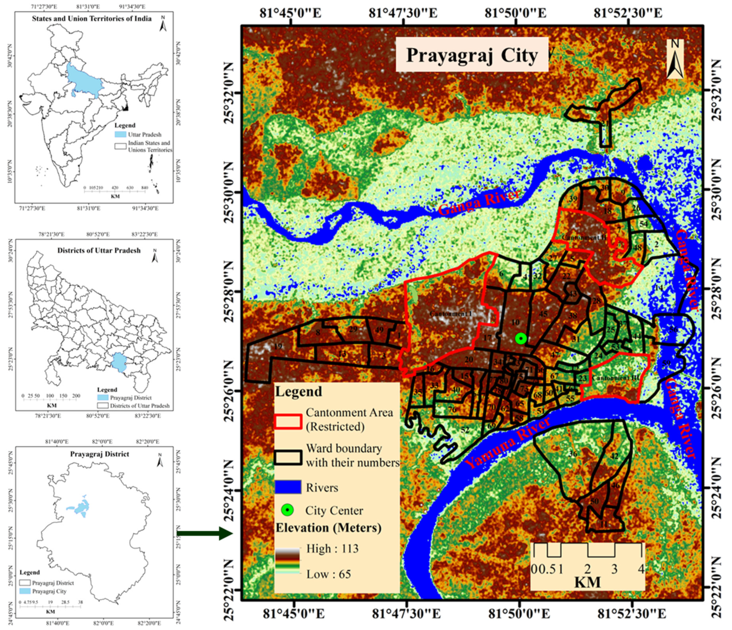
2.1. Study Area
2.2. Data Used
2.3. Methods
2.3.1. Land Indices
NDBI
EBBI
NDMI
NDVI
NDWI
SAVI
2.3.2. LST Retrieval
Landsat-Based LST Calculation
MODIS-Based Night-Time LST Calculation
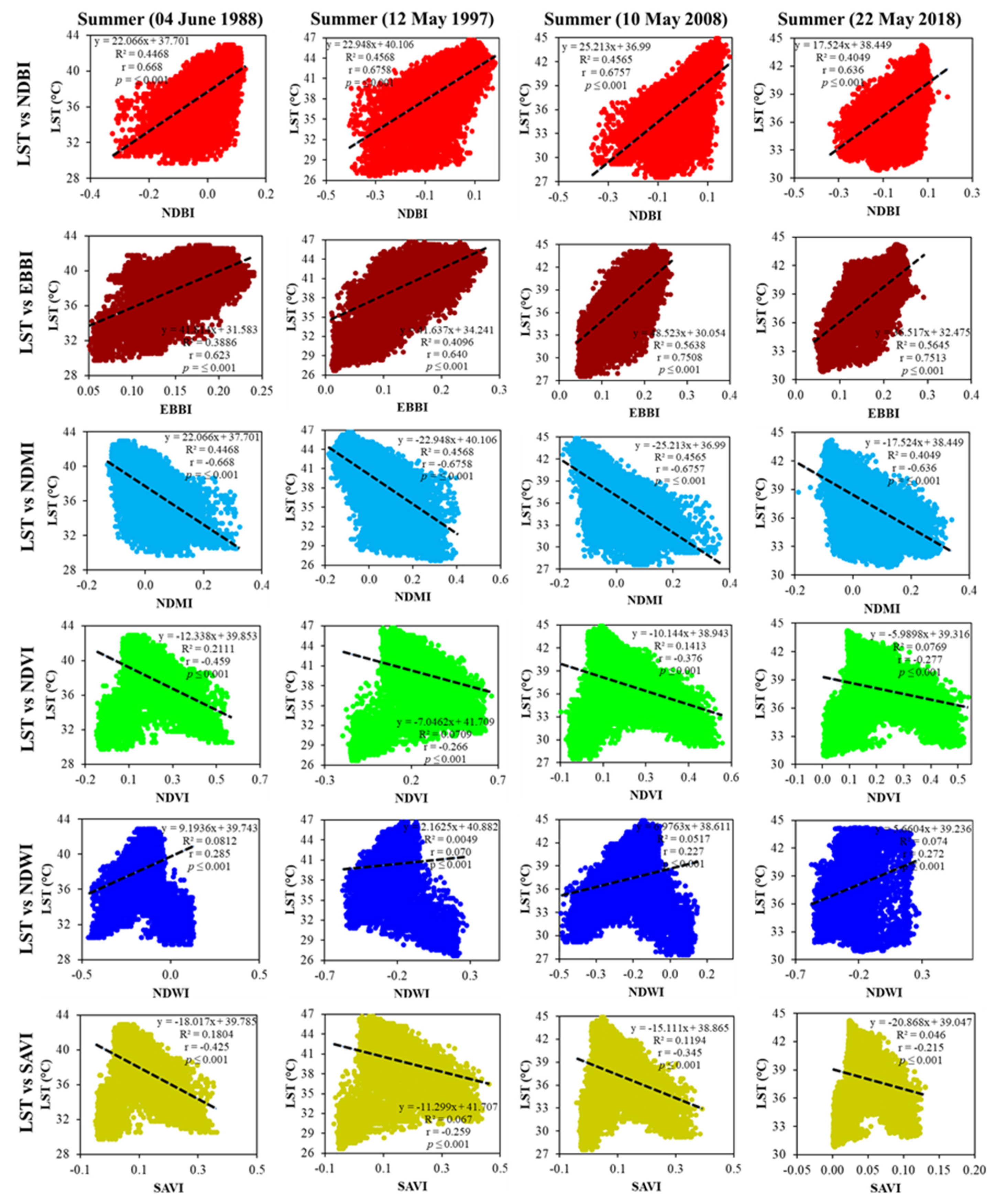
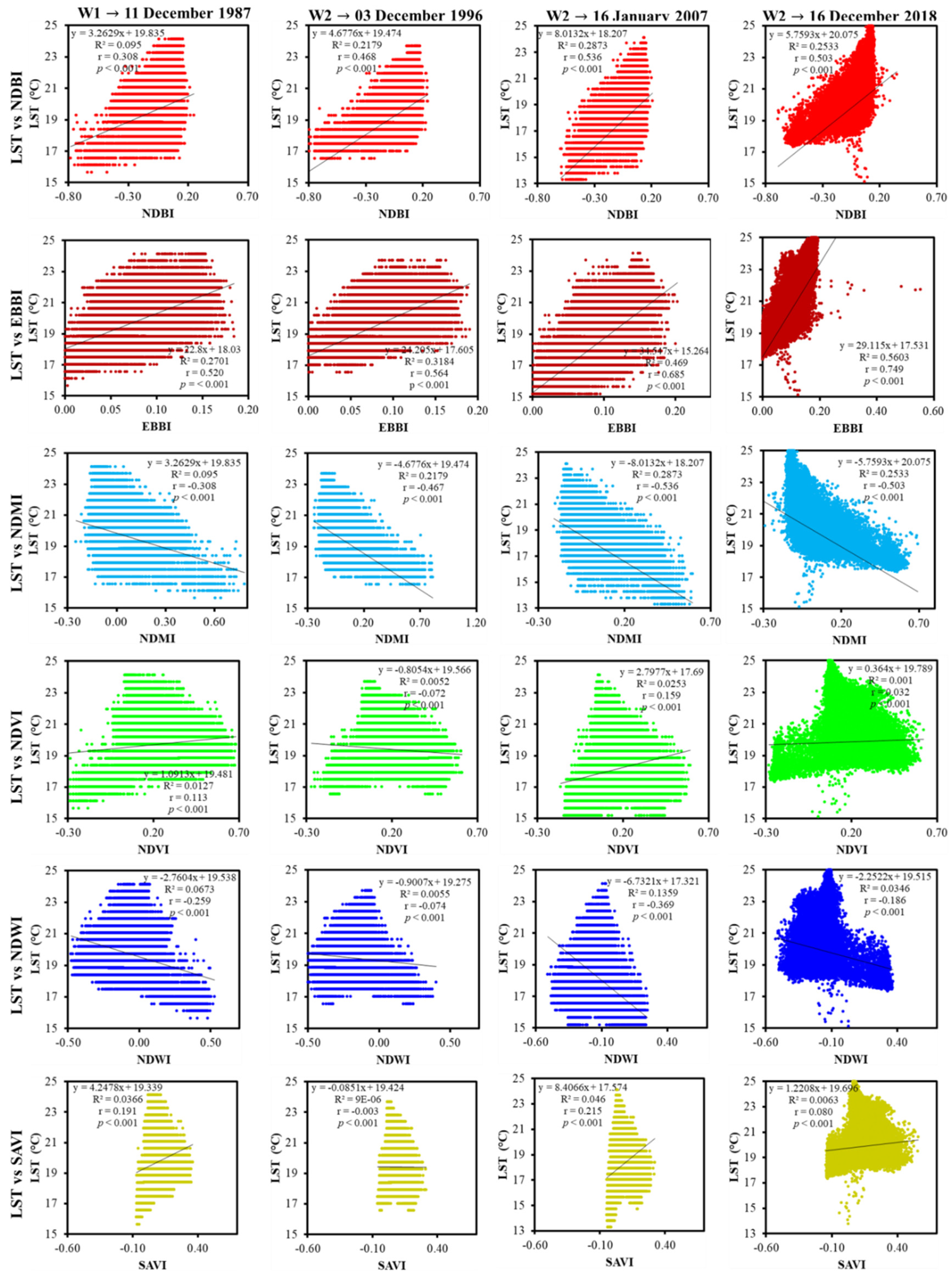
2.3.3. Influence of Land Indices on LST
2.3.4. Intensity of SUHI Calculation
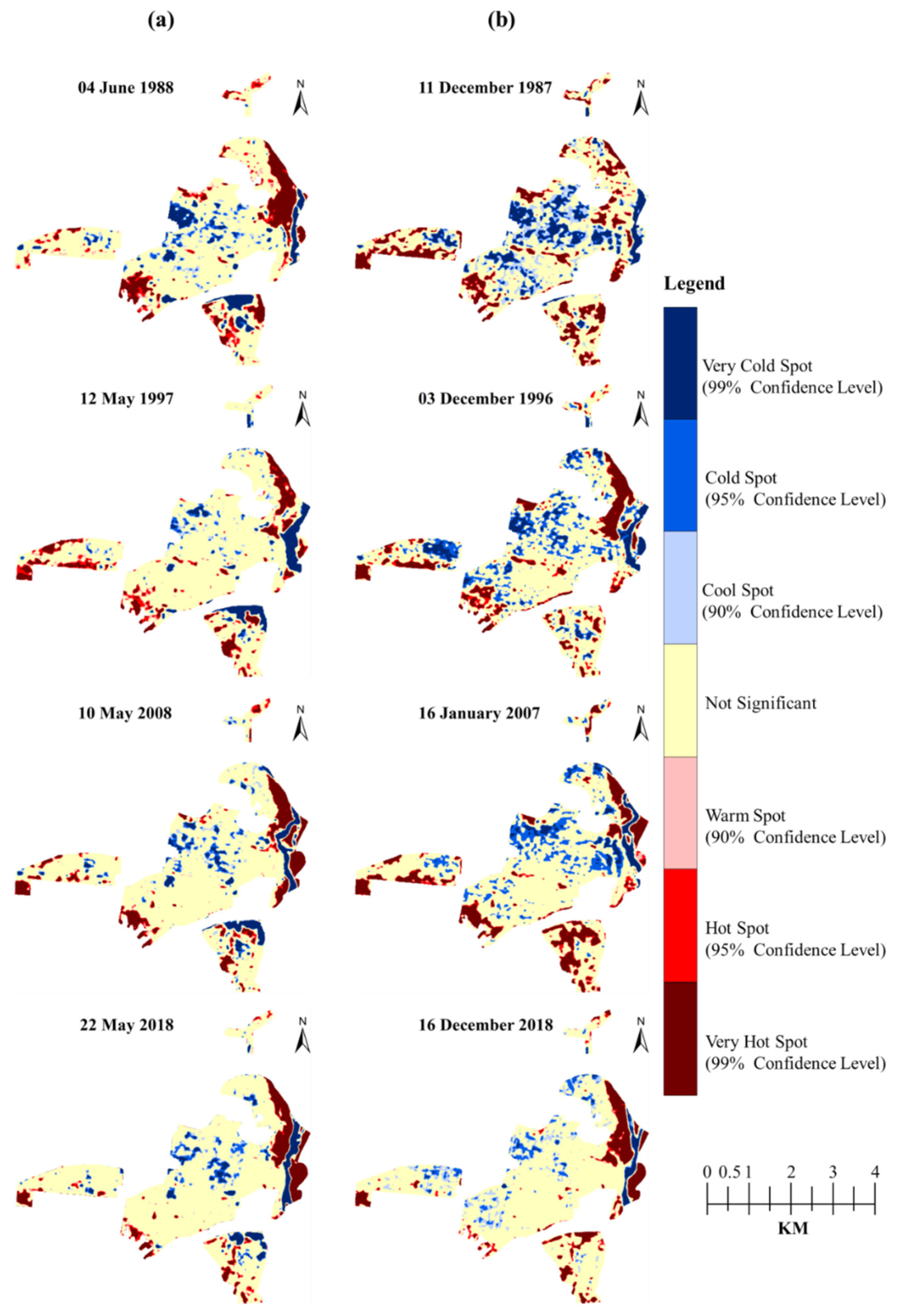
2.3.5. Hotspot Analysis (Getis–Ord Gi*)
3. Results
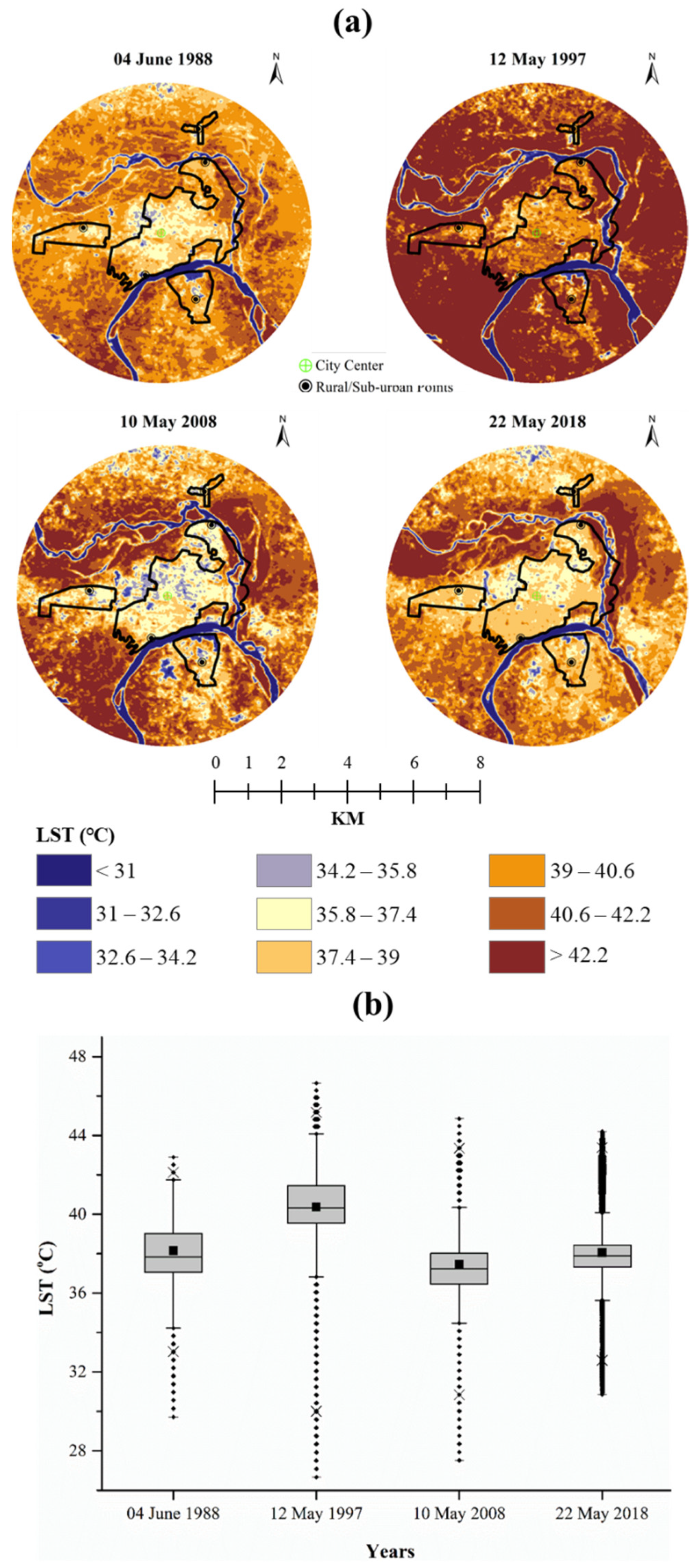
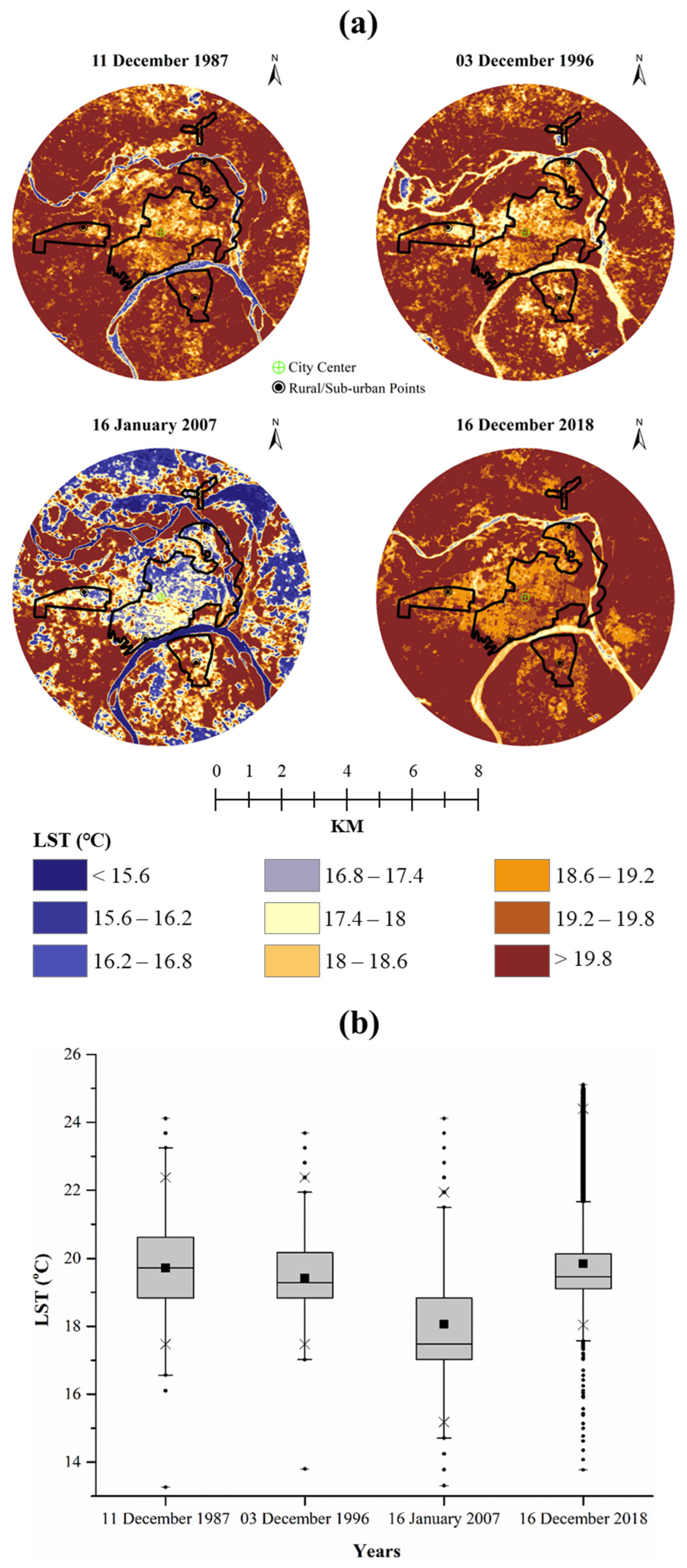
3.1. Seasonal Spatiotemporal LST Dynamics
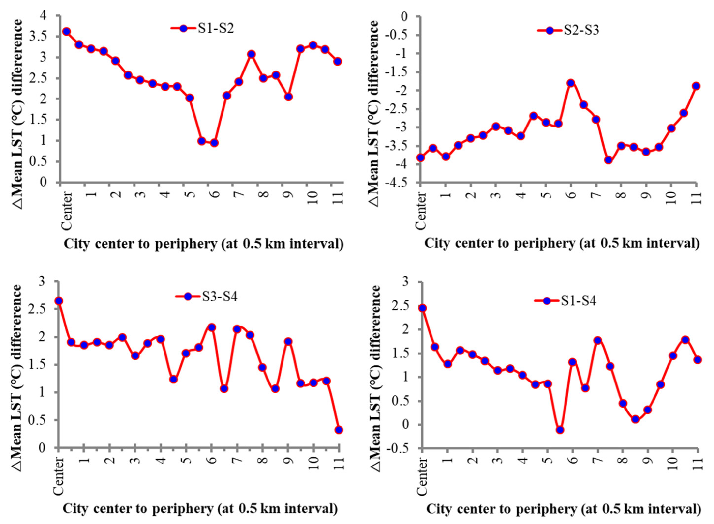
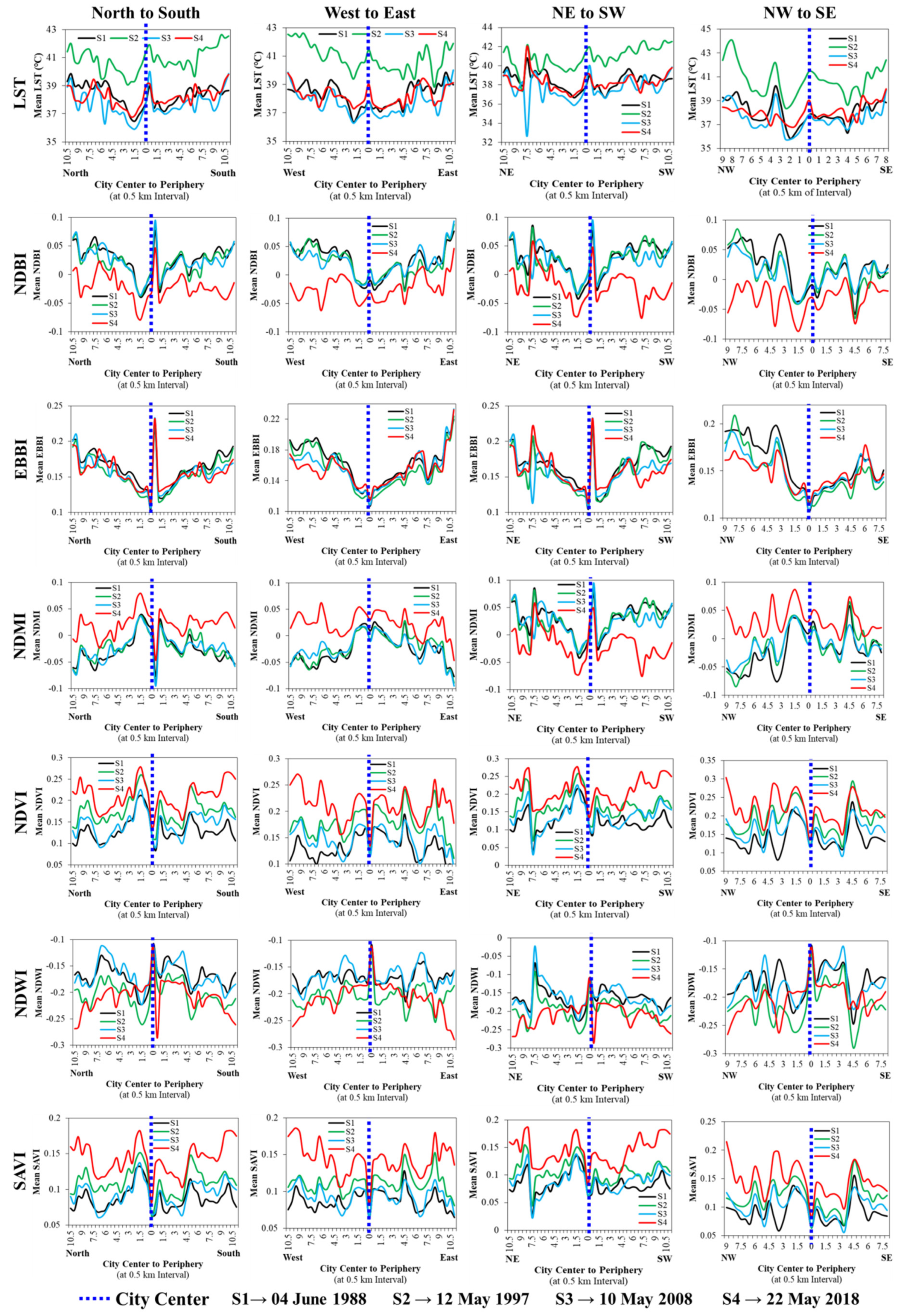
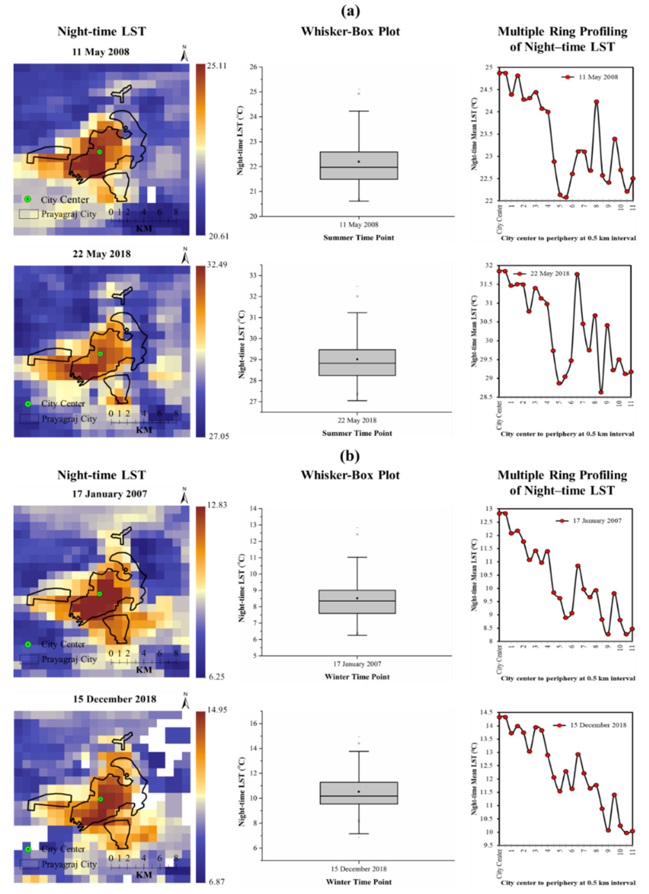
3.2. Seasonal Magnitude of LST Based on Multiple Ring Profiling
3.3. Spatiotemporal Dynamics of Land Indices and LST, and Their Relationships
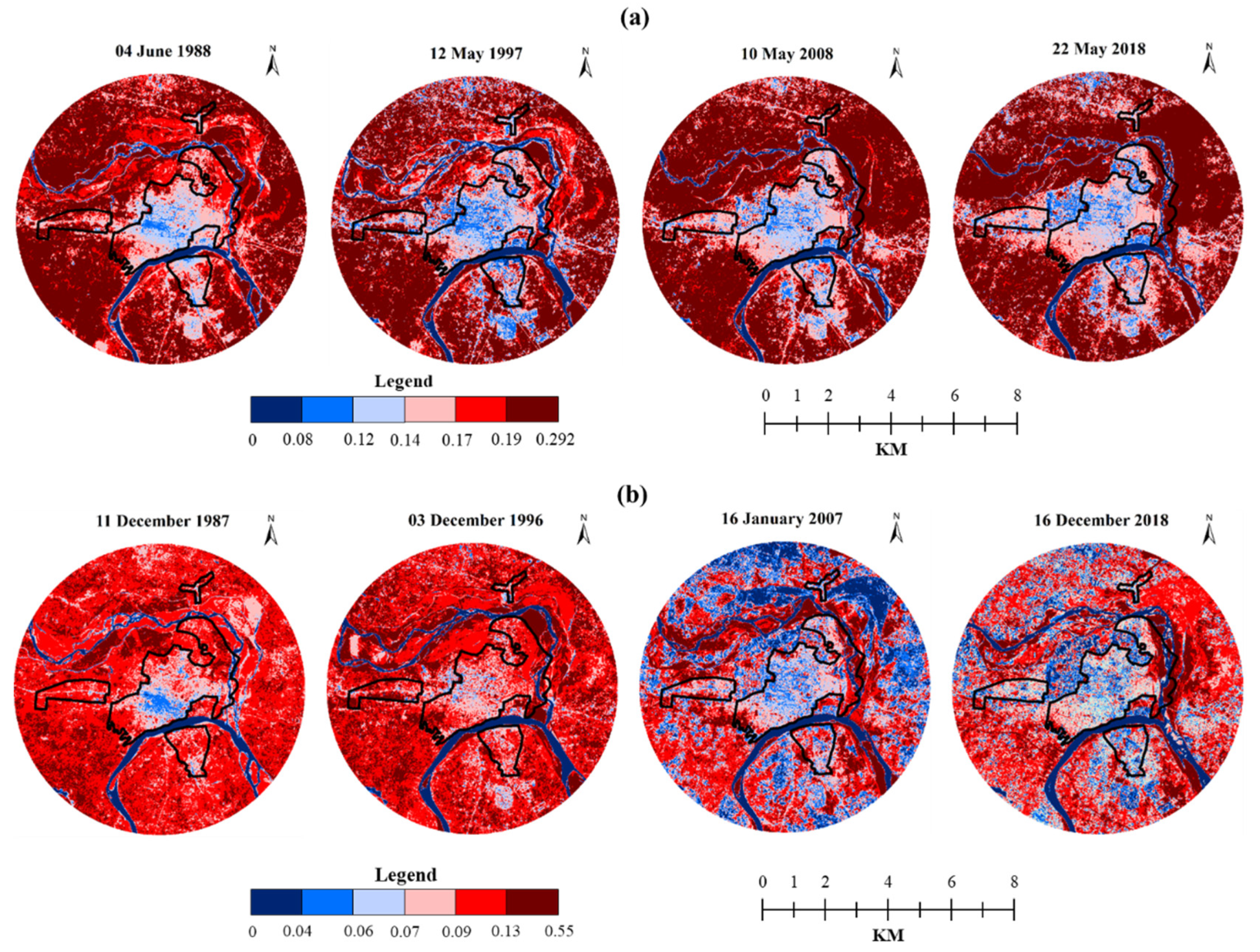
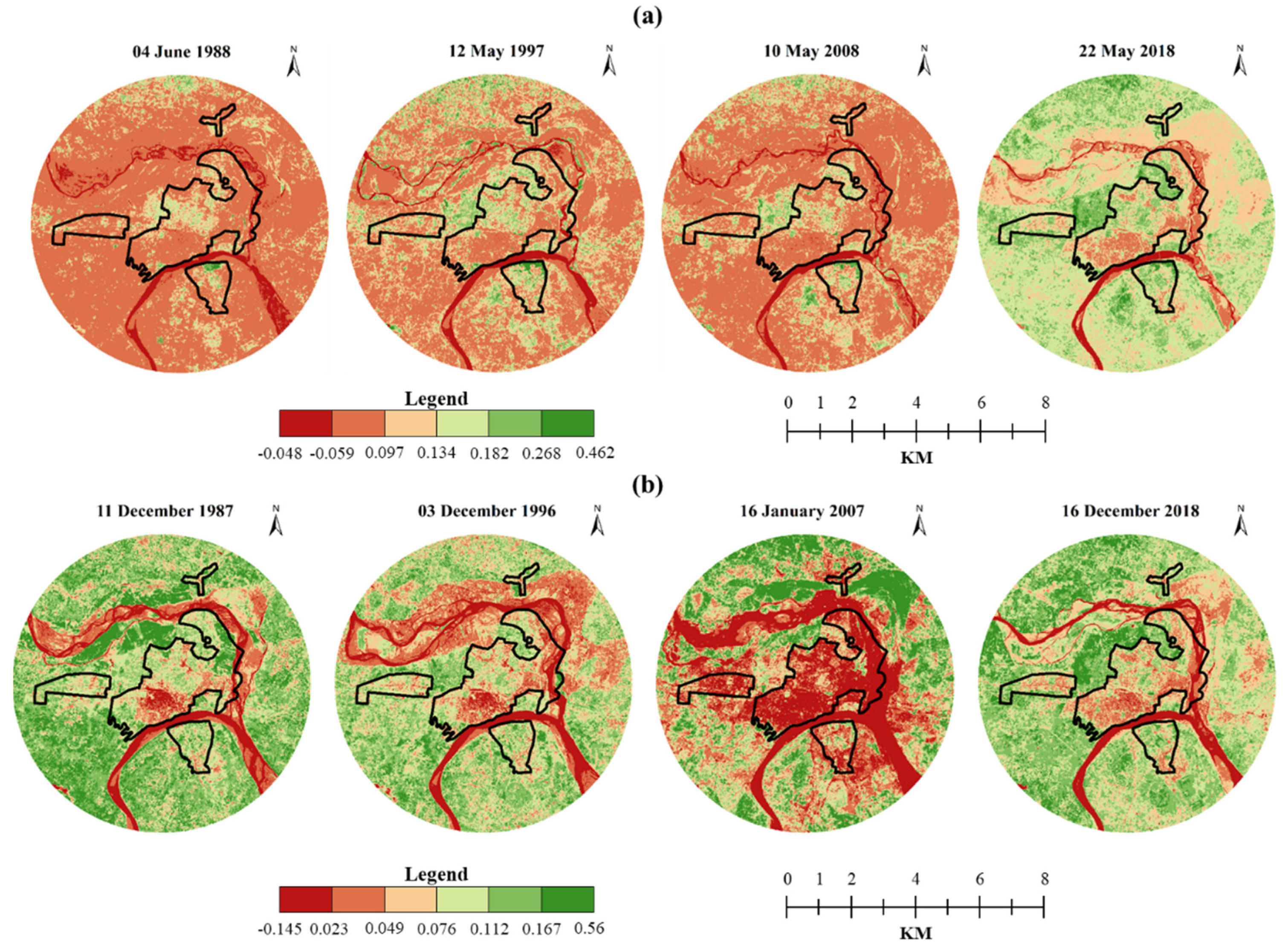
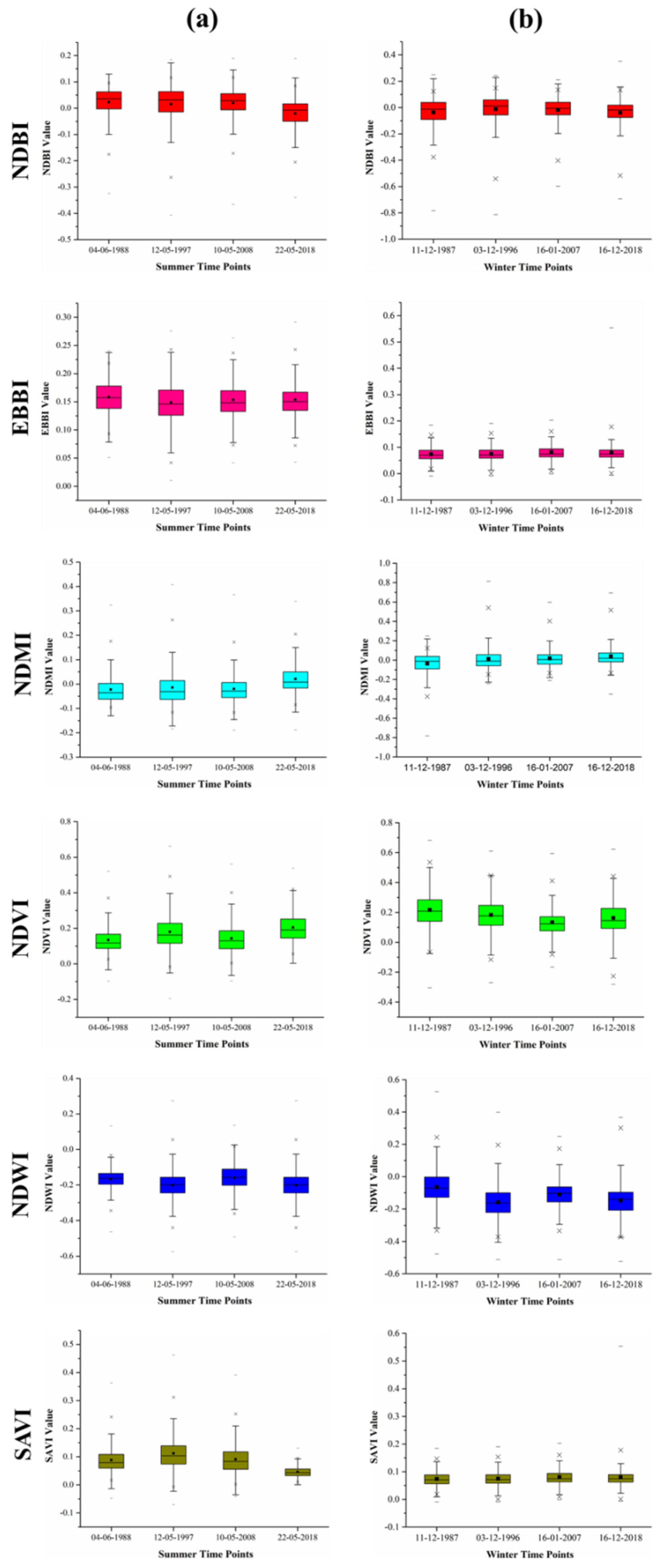
3.3.1. NDBI Dynamics and Its Connection with LST
3.3.2. EBBI Dynamics and Its Connection with LST
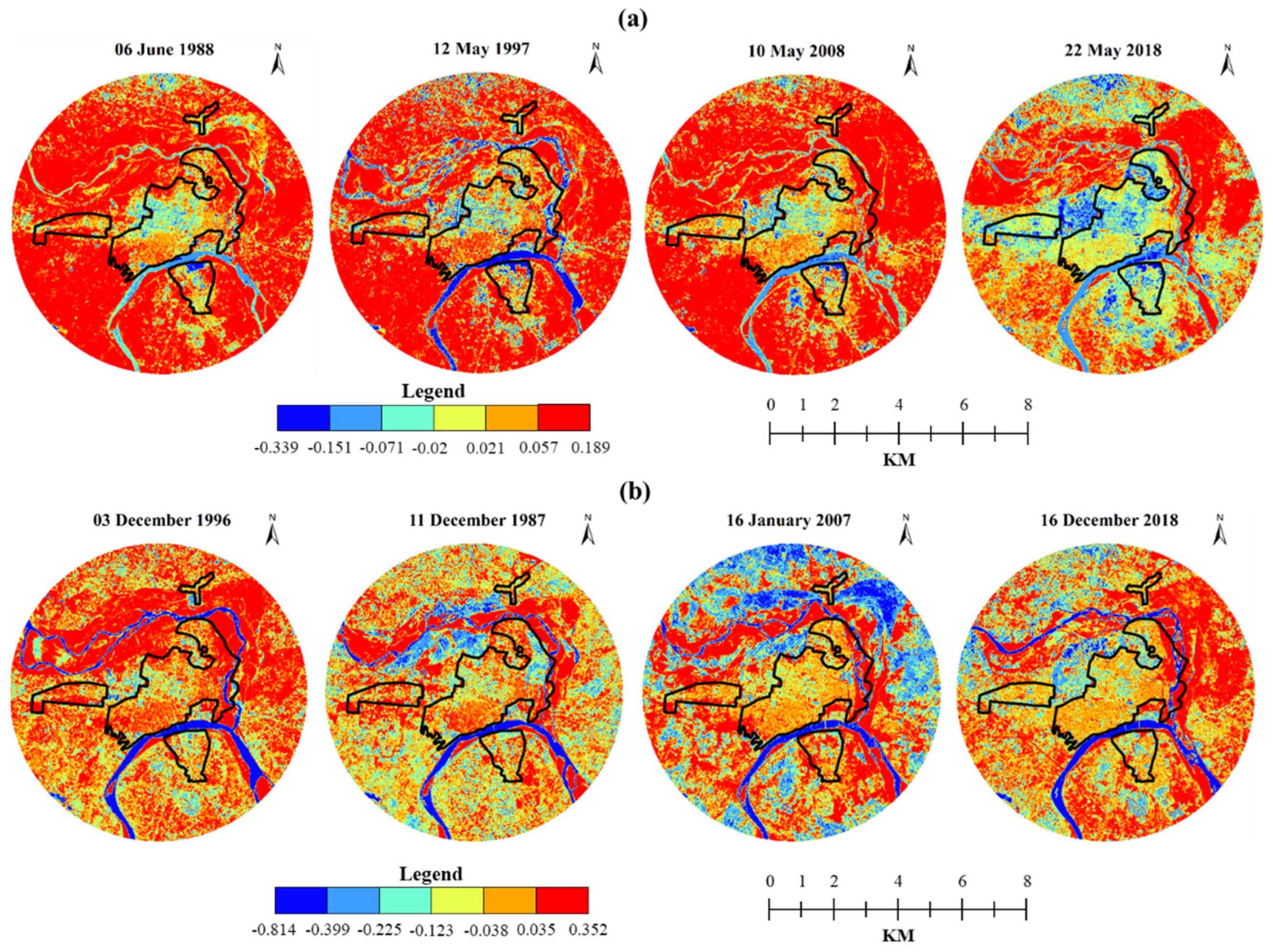
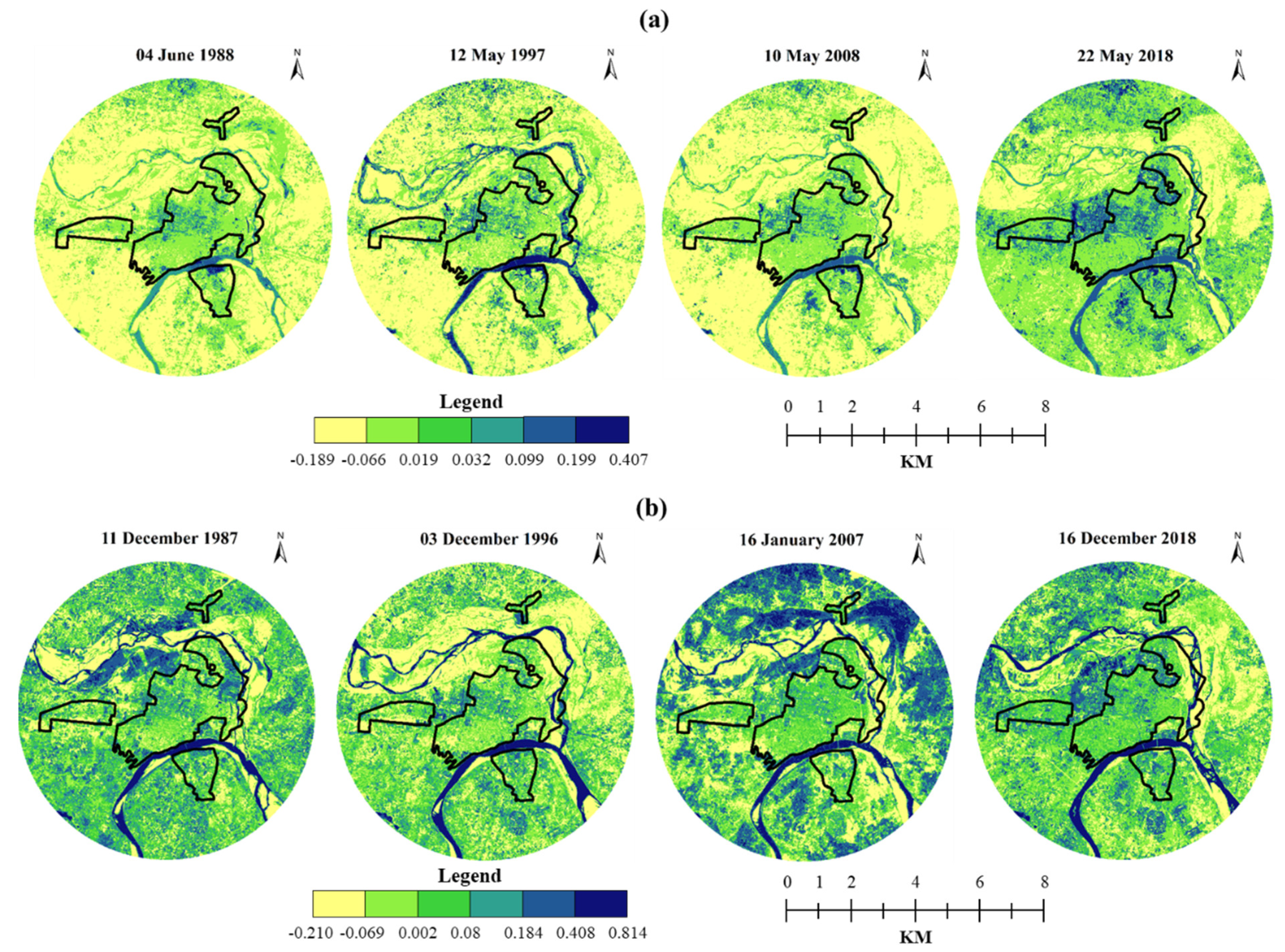
3.3.3. NDMI Dynamics and Its Relationship with LST
3.3.4. NDVI Dynamics and Its Relationship with LST
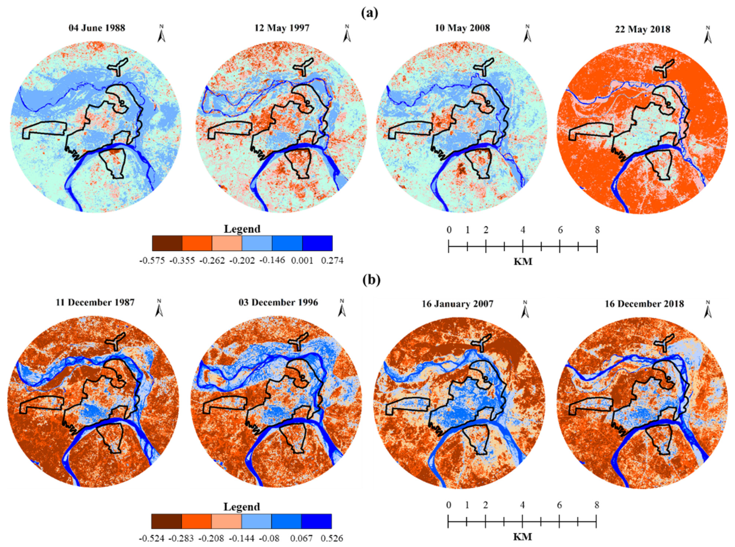
3.3.5. NDWI Dynamics and Its Relationship with LST
3.3.6. SAVI Dynamics and Its Relationship with LST
3.4. Effects of Land Indices on LST Distribution
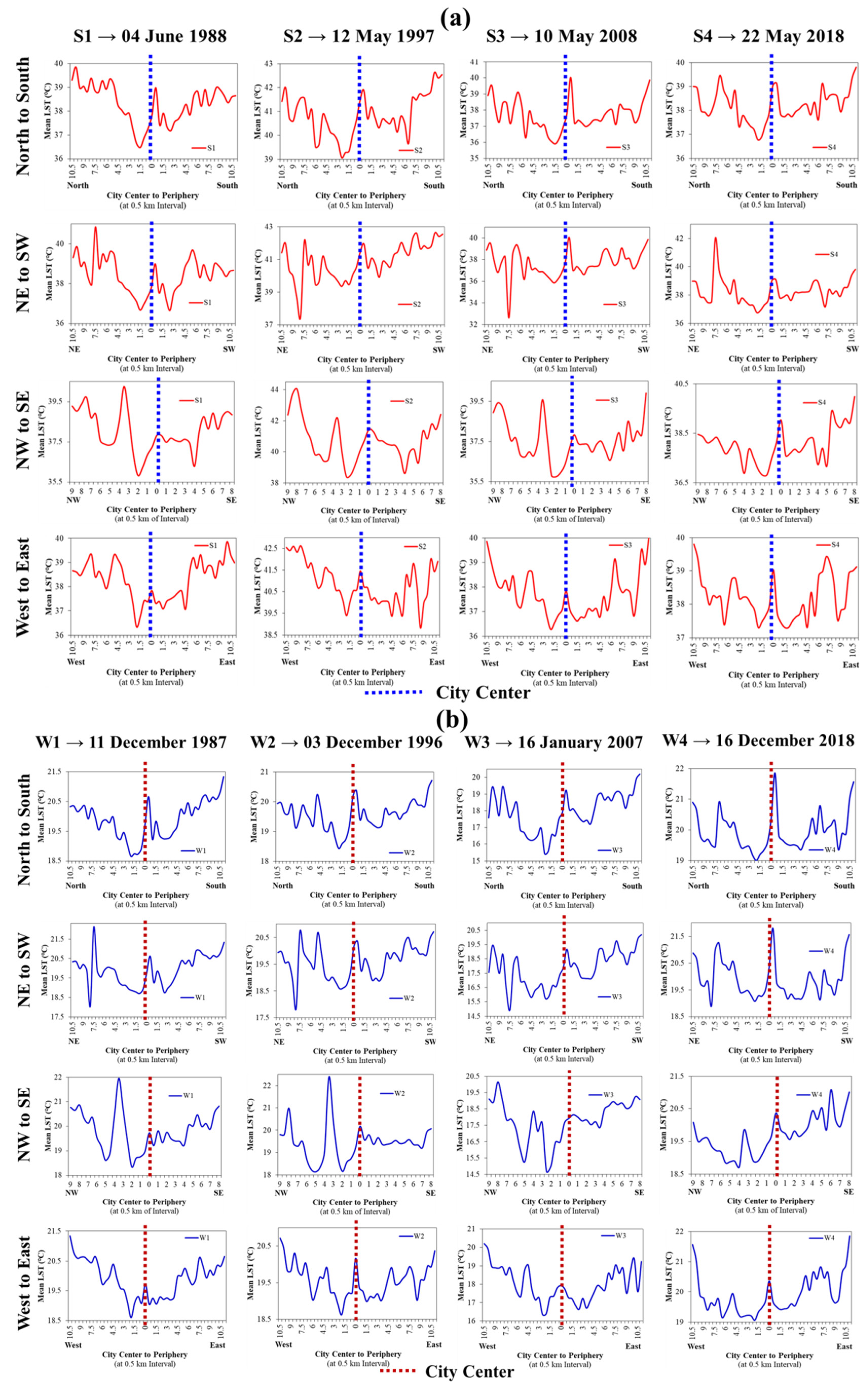
3.4.1. North to South
3.4.2. Northeast (NE) to Southwest (SW)
3.4.3. Northwest (NW) to Southeast (SE)
3.4.4. West to East
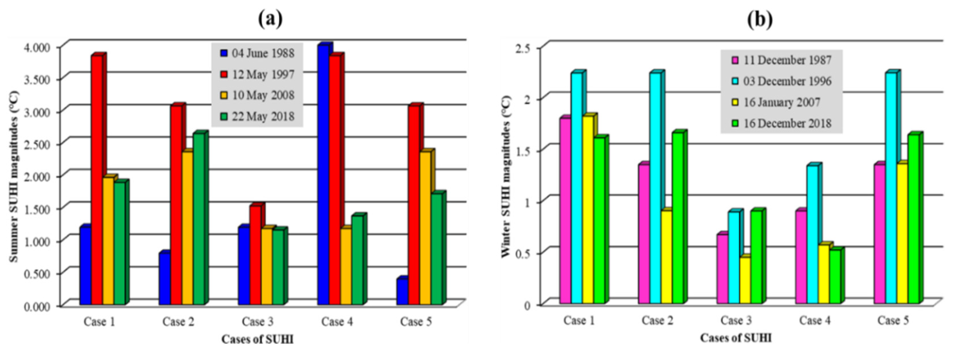
3.5. SUHI Dynamics
3.5.1. Urban and Rural/Suburban Point Location-Based SUHI
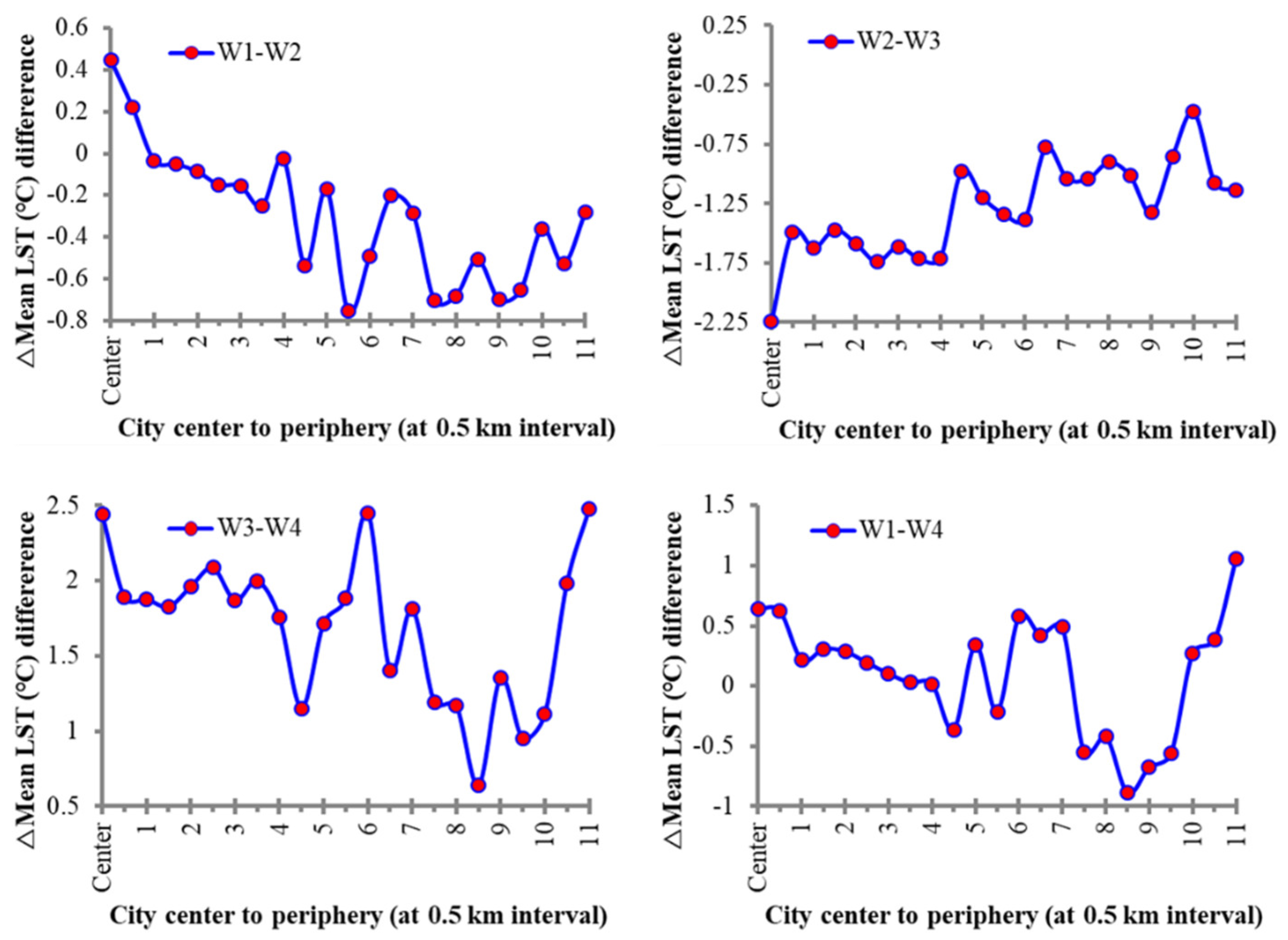
3.5.2. Directional Ring Profiling of LST for Investigation of SUHI
North to South
NE to SE
NW to SE
West to East
3.6. Hotspot Identification
4. Discussion
4.1. Urbanization: An Assessment for Effective Urban Planning
4.2. An Overview of Night-Time LST for SUHI Exploration
5. Conclusions
Supplementary Materials
Author Contributions
Funding
Data Availability Statement
Acknowledgments
Conflicts of Interest
Appendix A


References
- United Nations. The World’s Cities in 2018—Data Booklet (ST/ESA/SER.A/417); Department of Economic and Social Affairs, Population Division: New York, NY, USA, 2018; pp. 1–34. [Google Scholar]
- IPCC. Climate Change and Land. An IPCC Special Report on Climate Change, Desertification, Land Degradation, Sustainable Land Management, Food Security, and Greenhouse Gas Fluxes in Terrestrial Ecosystems. Summary for Policymakers; IPCC: Geneva, Switzerland, 2019. [Google Scholar]
- Rosa, A.; de Oliveira, F.S.; Gomes, A.; Gleriani, J.M.; Gonçalves, W.; Moreira, G.L.; Silva, F.G.; Ricardo, E.; Branco, F.; Moura, M.M.; et al. Spatial and Temporal Distribution of Urban Heat Islands. Sci. Total Environ. 2017, 605–606, 946–956. [Google Scholar] [CrossRef]
- Thomas, G.; Sherin, A.P.; Ansar, S.; Zachariah, E.J. Analysis of Urban Heat Island in Kochi, India, Using a Modified Local Climate Zone Classification. Procedia Environ. Sci. 2014, 21, 3–13. [Google Scholar] [CrossRef] [Green Version]
- IPCC. Climate Change 2021: The Physical Science Basis; IPCC: Geneva, Switzerland, 2021. [Google Scholar]
- Ranagalage, M.; Estoque, R.C.; Murayama, Y. An Urban Heat Island Study of the Colombo Metropolitan Area, Sri Lanka, Based on Landsat Data (1997–2017). ISPRS Int. J. Geo-Inf. 2017, 6, 189. [Google Scholar] [CrossRef] [Green Version]
- Son, N.T.; Chen, C.F.; Chen, C.R.; Thanh, B.X.; Vuong, T.H. Assessment of Urbanization and Urban Heat Islands in Ho Chi Minh City, Vietnam Using Landsat Data. Sustain. Cities Soc. 2017, 30, 150–161. [Google Scholar] [CrossRef]
- Liu, H.; Weng, Q. Seasonal Variations in the Relationship between Landscape Pattern and Land Surface Temperature in Indianapolis, USA. Environ. Monit. Assess. 2008, 144, 199–219. [Google Scholar] [CrossRef]
- Sultana, S.; Satyanarayana, A.N. V Urban Heat Island Intensity during Winter over Metropolitan Cities of India Using Remote-Sensing Techniques: Impact of Urbanization. Int. J. Remote Sens. 2018, 39, 6692–6730. [Google Scholar] [CrossRef]
- He, Y.; Lin, E.S.; Zhang, W.; Tan, C.L.; Tan, P.Y.; Wong, N.H. Local Microclimate above Shrub and Grass in Tropical City: A Case Study in Singapore. Urban Clim. 2022, 43, 101142. [Google Scholar] [CrossRef]
- Estoque, R.C.; Murayama, Y. Quantifying Landscape Pattern and Ecosystem Service Value Changes in Four Rapidly Urbanizing Hill Stations of Southeast Asia. Landsc. Ecol. 2016, 31, 1481–1507. [Google Scholar] [CrossRef]
- Dissanayake, D.; Morimoto, T.; Murayama, Y.; Ranagalage, M. Impact of Landscape Structure on the Variation of Land Surface Temperature in Sub-Saharan Region: A Case Study of Addis Ababa Using Landsat Data. Sustainability 2019, 11, 2257. [Google Scholar] [CrossRef] [Green Version]
- Rousta, I.; Sarif, M.O.; Gupta, R.D.; Olafsson, H.; Ranagalage, M.; Murayama, Y.; Zhang, H.; Mushore, T.D. Spatiotemporal Analysis of Land Use/Land Cover and Its Effects on Surface Urban Heat Island Using Landsat Data: A Case Study of Metropolitan City Tehran (1988–2018). Sustainability 2018, 10, 4433. [Google Scholar] [CrossRef]
- Sharma, R.; Chakraborty, A.; Joshi, P.K. Geospatial Quantification and Analysis of Environmental Changes in Urbanizing City of Kolkata (India). Environ. Monit. Assess. 2015, 187, 4206. [Google Scholar] [CrossRef] [PubMed]
- Chen, T.L.; Lin, Z.H. Impact of Land Use Types on the Spatial Heterogeneity of Extreme Heat Environments in a Metropolitan Area. Sustain. Cities Soc. 2021, 72, 103005. [Google Scholar] [CrossRef]
- Myint, S.W.; Brazel, A.; Okin, G.; Buyantuyev, A. Combined Effects of Impervious Surface and Vegetation Cover on Air Temperature Variations in a Rapidly Expanding Desert City. GIScience Remote Sens. 2010, 47, 301–320. [Google Scholar] [CrossRef]
- Faisal, A.A.; Kafy, A.-A.; Al Rakib, A.; Akter, K.S.; Jahir, D.M.A.; Sikdar, M.S.; Ashrafi, T.J.; Mallik, S.; Rahman, M.M. Assessing and Predicting Land Use/Land Cover, Land Surface Temperature and Urban Thermal Field Variance Index Using Landsat Imagery for Dhaka Metropolitan Area. Environ. Challenges 2021, 4, 100192. [Google Scholar] [CrossRef]
- Sarif, M.O.; Rimal, B.; Stork, N.E. Assessment of Changes in Land Use/Land Cover and Land Surface Temperatures and Their Impact on Surface Urban Heat Island Phenomena in the Kathmandu Valley (1988–2018). ISPRS Int. J. Geo-Inf. 2020, 9, 726. [Google Scholar] [CrossRef]
- Kong, F.; Yin, H.; James, P.; Hutyra, L.R.; He, H.S. Effects of Spatial Pattern of Greenspace on Urban Cooling in a Large Metropolitan Area of Eastern China. Landsc. Urban Plan. 2014, 128, 35–47. [Google Scholar] [CrossRef]
- Li, L.; Zha, Y.; Zhang, J. Spatial and Dynamic Perspectives on Surface Urban Heat Island and Their Relationships with Vegetation Activity in Beijing, China, Based on Moderate Resolution Imaging Spectroradiometer Data. Int. J. Remote Sens. 2020, 41, 882–896. [Google Scholar] [CrossRef]
- Wang, R.; Derdouri, A.; Murayama, Y. Spatiotemporal Simulation of Future Land Use/Cover Change Scenarios in the Tokyo Metropolitan Area. Sustainability 2018, 10, 2056. [Google Scholar] [CrossRef] [Green Version]
- Ward, K.; Lauf, S.; Kleinschmit, B.; Endlicher, W. Heat Waves and Urban Heat Islands in Europe: A Review of Relevant Drivers. Sci. Total Environ. 2016, 569–570, 527–539. [Google Scholar] [CrossRef]
- Liu, L.; Zhang, Y. Urban Heat Island Analysis Using the Landsat TM Data and ASTER Data: A Case Study in Hong Kong. Remote Sens. 2011, 3, 1535–1552. [Google Scholar] [CrossRef]
- Tang, J.; Di, L.; Xiao, J.; Lu, D.; Zhou, Y. Impacts of Land Use and Socioeconomic Patterns on Urban Heat Island. Int. J. Remote Sens. 2017, 38, 3445–3465. [Google Scholar] [CrossRef]
- Abutaleb, K.; Ngie, A.; Darwish, A.; Ahmed, M.; Arafat, S.; Ahmed, F. Assessment of Urban Heat Island Using Remotely Sensed Imagery over Greater Cairo, Egypt. Adv. Remote Sens. 2015, 4, 35–47. [Google Scholar] [CrossRef] [Green Version]
- Ghosh, S.; Chatterjee, N.D.; Dinda, S. Relation between Urban Biophysical Composition and Dynamics of Land Surface Temperature in the Kolkata Metropolitan Area: A GIS and Statistical Based Analysis for Sustainable Planning. Model. Earth Syst. Environ. 2018, 5, 307–329. [Google Scholar] [CrossRef]
- Grover, A.; Singh, R.B. Analysis of Urban Heat Island (UHI) in Relation to Normalized Difference Vegetation Index (NDVI): A Comparative Study of Delhi and Mumbai. Environments 2015, 2, 125–138. [Google Scholar] [CrossRef] [Green Version]
- Sultana, S.; Satyanarayana, A.N.V. Assessment of Urbanisation and Urban Heat Island Intensities Using Landsat Imageries during 2000–2018 over a Sub-Tropical Indian City. Sustain. Cities Soc. 2020, 52, 101846. [Google Scholar] [CrossRef]
- Chakraborti, S.; Banerjee, A.; Sannigrahi, S.; Pramanik, S.; Maiti, A.; Jha, S. Assessing the Dynamic Relationship among Land Use Pattern and Land Surface Temperature: A Spatial Regression Approach. Asian Geogr. 2019, 36, 93–116. [Google Scholar] [CrossRef]
- Singh, P.; Kikon, N.; Verma, P. Impact of Land Use Change and Urbanization on Urban Heat Island in Lucknow City, Central India: A Remote Sensing Based Estimate. Sustain. Cities Soc. 2017, 32, 100–114. [Google Scholar] [CrossRef]
- Sarif, M.O.; Gupta, R.D. Land Surface Temperature Profiling and Its Relationships with Land Indices: A Case Study on Lucknow City. In ISPRS Annals of Photogrammetry, Remote Sensing and Spatial Information Sciences; Copernicus Publications: Dhulikhel, Nepal, 2019; Volume IV-5/W2, pp. 89–96. [Google Scholar]
- Guha, S.; Govil, H.; Mukherjee, S. Dynamic Analysis and Ecological Evaluation of Urban Heat Islands in Raipur City, India. J. Appl. Remote Sens. 2017, 11, 036020. [Google Scholar] [CrossRef]
- Mal, S.; Rani, S.; Maharana, P. Estimation of Spatio-Temporal Variability in Land Surface Temperature over the Ganga River Basin Using MODIS Data. Geocarto Int. 2020, 37, 3817–3839. [Google Scholar] [CrossRef]
- Shahfahad; Naikoo, M.W.; Islam, A.R.M.T.; Mallick, J.; Rahman, A. Land Use/Land Cover Change and Its Impact on Surface Urban Heat Island and Urban Thermal Comfort in a Metropolitan City. Urban Clim. 2022, 41, 101052. [Google Scholar] [CrossRef]
- Mandal, J.; Patel, P.P.; Samanta, S. Examining the Expansion of Urban Heat Island Effect in the Kolkata Metropolitan Area and Its Vicinity Using Multi-Temporal MODIS Satellite Data. Adv. Sp. Res. 2022, 69, 1960–1977. [Google Scholar] [CrossRef]
- Barat, A.; Parth Sarthi, P.; Kumar, S.; Kumar, P.; Sinha, A.K. Surface Urban Heat Island (SUHI) Over Riverside Cities Along the Gangetic Plain of India. Pure Appl. Geophys. 2021, 178, 1477–1497. [Google Scholar] [CrossRef]
- UN-Habitat. Tracking Progress Towards Inclusive, Safe, Resilient and Sustainable Cities and Human Settlements; United Nations: New York, NY, USA, 2018. [Google Scholar]
- Fonji, S.F.; Taff, G.N. Using Satellite Data to Monitor Land-Use Land-Cover Change in North-Eastern Latvia. Springerplus 2014, 3, 61. [Google Scholar] [CrossRef] [PubMed] [Green Version]
- MoHUA. Smart Citie: Ministry of Housing and Urban Affairs Reports, Government of India; MoHUA: New Delhi, India, 2015. [Google Scholar]
- PNN. Prayag Kumbh. Prayagraj Nagar Nigam, Government of Uttar Pradesh. Available online: allahabadmc.gov.in/kumbh_mela.html (accessed on 22 October 2019).
- Singh, S.K.; Mustak, S.; Srivastava, P.K.; Szabó, S.; Islam, T. Predicting Spatial and Decadal LULC Changes Through Cellular Automata Markov Chain Models Using Earth Observation Datasets and Geo-Information. Environ. Process. 2015, 2, 61–78. [Google Scholar] [CrossRef] [Green Version]
- Chaturvedi, R. Application of Remote Sensing and GIS in Land Use/Land Covers Mapping in Allahabad District. Int. J. Adv. Inf. Eng. Technol. 2014, 4, 1–9. [Google Scholar]
- Nanda, M.K. Climatic Classification. In Environmental Science; Khan, D.K., Ed.; e-Pathsala: New Delhi, India, 2018; pp. 1–16. [Google Scholar]
- IMD. Allahabad Climatological Table (Period: 1981–2010). Indian Meteorological Department, Government of India. Available online: http://www.imd.gov.in/section/climate/extreme/allahabad2.htm (accessed on 22 October 2019).
- Sobrino, J.A.; Jiménez-Muñoz, J.C.; Paolini, L. Land Surface Temperature Retrieval from LANDSAT TM 5. Remote Sens. Environ. 2004, 90, 434–440. [Google Scholar] [CrossRef]
- Lu, Y.; He, T.; Xu, X.; Qiao, Z. Investigation the Robustness of Standard Classification Methods for Defining Urban Heat Islands. IEEE J. Sel. Top. Appl. Earth Obs. Remote Sens. 2021, 14, 11386–11394. [Google Scholar] [CrossRef]
- Renard, F.; Alonso, L.; Fitts, Y.; Hadjiosif, A.; Comby, J. Evaluation of the Effect of Urban Redevelopment on Surface Urban Heat Islands. Remote Sens. 2019, 11, 299. [Google Scholar] [CrossRef] [Green Version]
- Haque, M.I.; Basak, R. Land Cover Change Detection Using GIS and Remote Sensing Techniques: A Spatio-Temporal Study on Tanguar Haor, Sunamganj, Bangladesh. Egypt. J. Remote Sens. Sp. Sci. 2017, 20, 251–263. [Google Scholar] [CrossRef]
- Hasanlou, M.; Mostofi, N. Investigating Urban Heat Island Estimation and Relation between Various Land Cover Indices in Tehran City Using Landsat 8 Imagery. In Proceedings of the 1st International Electronic Conference on Remote sensing, Basel, Switzerland, 22 June–5 July 2015; MDPI: Basel, Switzerland, 2015; pp. 1–11. [Google Scholar]
- Qin, Z.; Karnieli, A.; Berliner, P. A Mono-Window Algorithm for Retrieving Land Surface Temperature from Landsat TM Data and Its Application to the Israel-Egypt Border Region. Int. J. Remote Sens. 2001, 22, 3719–3746. [Google Scholar] [CrossRef]
- Zhu, X.; Duan, S.B.; Li, Z.L.; Zhao, W.; Wu, H.; Leng, P.; Gao, M.; Zhou, X. Retrieval of Land Surface Temperature with Topographic Effect Correction from Landsat 8 Thermal Infrared Data in Mountainous Areas. IEEE Trans. Geosci. Remote Sens. 2021, 59, 6674–6687. [Google Scholar] [CrossRef]
- Yang, L.; Cao, Y.; Zhu, X.; Zeng, S.; Yang, G.; He, J.; Yang, X. Land Surface Temperature Retrieval for Arid Regions Based on Landsat-8 TIRS Data: A Case Study in Shihezi, Northwest China. J. Arid Land 2014, 6, 704–716. [Google Scholar] [CrossRef] [Green Version]
- Shahfahad; Kumari, B.; Tayyab, M.; Ahmed, I.A.; Baig, M.R.I.; Khan, M.F.; Rahman, A. Longitudinal Study of Land Surface Temperature (LST) Using Mono- and Split-Window Algorithms and Its Relationship with NDVI and NDBI over Selected Metro Cities of India. Arab. J. Geosci. 2020, 13, 1040. [Google Scholar] [CrossRef]
- Wang, L.; Lu, Y.; Yao, Y. Comparison of Three Algorithms for the Retrieval of Land Surface Temperature from Landsat 8 Images. Sensors 2019, 19, 5049. [Google Scholar] [CrossRef] [PubMed] [Green Version]
- Jiménez-Munoz, J.C.; Sobrino, J.A. A Generalized Single-Channel Method for Retrieving Land Surface Temperature from Remote Sensing Data. J. Geophys. Res. Atmos. 2004, 108, 1–9. [Google Scholar] [CrossRef] [Green Version]
- Rozenstein, O.; Qin, Z.; Derimian, Y.; Karnieli, A. Derivation of Land Surface Temperature for Landsat-8 TIRS Using a Split Window Algorithm. Sensors 2014, 14, 5768–5780. [Google Scholar] [CrossRef]
- Guha, S.; Govil, H. Annual Assessment on the Relationship between Land Surface Temperature and Six Remote Sensing Indices Using Landsat Data from 1988 to 2019. Geocarto Int. 2021, 37, 4292–4311. [Google Scholar] [CrossRef]
- Majumder, A.; Setia, R.; Kingra, P.K.; Sembhi, H.; Singh, S.P.; Pateriya, B. Estimation of Land Surface Temperature Using Different Retrieval Methods for Studying the Spatiotemporal Variations of Surface Urban Heat and Cold Islands in Indian Punjab. Environ. Dev. Sustain. 2021, 23, 15921–15942. [Google Scholar] [CrossRef]
- Guha, S.; Govil, H. An Assessment on the Relationship between Land Surface Temperature and Normalized Difference Vegetation Index. Environ. Dev. Sustain. 2021, 23, 1944–1963. [Google Scholar] [CrossRef]
- Nimish, G.; Bharath, H.A.; Lalitha, A. Exploring Temperature Indices by Deriving Relationship between Land Surface Temperature and Urban Landscape. Remote Sens. Appl. Soc. Environ. 2020, 18, 100299. [Google Scholar] [CrossRef]
- Sekertekin, A.; Bonafoni, S. Land Surface Temperature Retrieval from Landsat 5, 7, and 8 over Rural Areas: Assessment of Different Retrieval Algorithms and Emissivity Models and Toolbox Implementation. Remote Sens. 2020, 12, 294. [Google Scholar] [CrossRef]
- Kikon, N.; Singh, P.; Singh, S.K.; Vyas, A. Assessment of Urban Heat Islands (UHI) of Noida City, India Using Multi-Temporal Satellite Data. Sustain. Cities Soc. 2016, 22, 19–28. [Google Scholar] [CrossRef]
- Ziaul, S.; Pal, S. Image Based Surface Temperature Extraction and Trend Detection in an Urban Area of West Bengal, India. J. Environ. Geogr. 2016, 9, 13–25. [Google Scholar] [CrossRef] [Green Version]
- Oke, T.R.; East, C. The Urban Boundary Layer in Montreal. Bound.-Lay. Meteorol. 1971, 1, 411–437. [Google Scholar] [CrossRef]
- Oke, T.R. City Size and the Urban Heat Island. Atmos. Environ. 1973, 7, 769–779. [Google Scholar] [CrossRef]
- Tran, D.X.; Pla, F.; Latorre-Carmona, P.; Myint, S.W.; Caetano, M.; Kieu, H.V. Characterizing the Relationship between Land Use Land Cover Change and Land Surface Temperature. ISPRS J. Photogramm. Remote Sens. 2017, 124, 119–132. [Google Scholar] [CrossRef] [Green Version]
- Sarif, M.O.; Gupta, R.D. Spatiotemporal Mapping of Land Use/Land Cover Dynamics Using Remote Sensing and GIS Approach: A Case Study of Prayagraj City, India (1988–2018). Environ. Dev. Sustain. 2022, 24, 888–920. [Google Scholar] [CrossRef]
- Karakuş, C.B. The Impact of Land Use/Land Cover (LULC) Changes on Land Surface Temperature in Sivas City Center and Its Surroundings and Assessment of Urban Heat Island. Asia-Pac. J. Atmos. Sci. 2019, 55, 669–684. [Google Scholar] [CrossRef]
- Barat, A.; Kumar, S.; Kumar, P.; Sarthi, P.P. Characteristics of Surface Urban Heat Island (SUHI) over the Gangetic Plain of Bihar, India. Asia-Pacific J. Atmos. Sci. 2018, 54, 205–214. [Google Scholar] [CrossRef]
- Chen, R.; You, X. Reduction of Urban Heat Island and Associated Greenhouse Gas Emissions. Mitig. Adapt. Strateg. Glob. Chang. 2019, 25, 689–711. [Google Scholar] [CrossRef]
- Hien, W.N.; Tan, P.Y.; Yu, C. Study of Thermal Performance of Extensive Rooftop Greenery Systems in the Tropical Climate. Build. Environ. 2007, 42, 25–54. [Google Scholar] [CrossRef]
- Sen, S.; Roesler, J.; Ruddell, B.; Middel, A. Cool Pavement Strategies for Urban Heat Island Mitigation in Suburban Phoenix, Arizona. Sustainability 2019, 11, 4452. [Google Scholar] [CrossRef] [Green Version]
- Estoque, R.C.; Estoque, R.S.; Murayama, Y. Prioritizing Areas for Rehabilitation by Monitoring Change in Barangay-Based Vegetation Cover. ISPRS Int. J. Geo-Inf. 2012, 1, 46–68. [Google Scholar] [CrossRef] [Green Version]
- Simwanda, M.; Ranagalage, M.; Estoque, R.C.; Murayama, Y. Spatial Analysis of Surface Urban Heat Islands in Four Rapidly Growing African Cities. Remote Sens. 2019, 11, 1645. [Google Scholar] [CrossRef]


| Satellite (Sensor)/Ancillary Data | Path/Row | Resolution/Scale | Season | Acquisition Date | Time (GMT) | Constants of Thermal Conversion | Source | |
|---|---|---|---|---|---|---|---|---|
| K1 | K2 | |||||||
| Landsat-5 (TM) | 143/42 | 30 m | Summer | 04-06-1988 | 04:31:36 | 607.76 (Band 6) | 1260.56 (Band 6) | United States Geological Survey (USGS) web portal (https://earthexplorer.usgs.gov/, accessed on 15 January 2019) |
| 12-05-1997 | 04:29:21 | 607.76 (Band 6) | 1260.56 (Band 6) | |||||
| 10-05-2008 | 04:49:45 | 607.76 (Band 6) | 1260.56 (Band 6) | |||||
| Landsat-8 (OLI/TIRS) | 22-05-2018 | 05:00:01 | 774.8853 (Band 10) | 1321.0789 (Band 10) | ||||
| Landsat-5 (TM) | 143/42 | 30 m | Winter | 11-12-1987 | 04:29:34 | 607.76 (Band 6) | 1260.56 (Band 6) | |
| 03-12-1996 | 04:22:45 | 607.76 (Band 6) | 1260.56 (Band 6) | |||||
| 16-01-2007 | 04:55:59 | 607.76 (Band 6) | 1260.56 (Band 6) | |||||
| Landsat-8 (OLI/TIRS) | 16-12-2018 | 05:00:58 | 480.8883 (Band 11) | 1201.1442 (Band 11) | ||||
| MODIS (Terra) | - | 1 km | Summer | 11-05-2008 | Night–time | - | - | |
| - | 22-05-2018 | - | - | |||||
| - | 1 km | Winter | 17-01-2007 | - | - | |||
| - | 15-12-2018 | - | - | |||||
| ASTER | - | 30 m | - | 13-09-2017 | - | - | - | |
| Ward boundary map | - | 1:21,600 | - | - | - | - | - | Prayagraj Nagar Nigam |
| Political map | - | 1:4 M | - | 2014 | - | - | - | Survey of India |
| Atmospheric Profile | Water Vapor (w) (g/cm2) | Equation for Transmittance Estimation | Squared Correlation (R2) | Standard Error |
|---|---|---|---|---|
| High air temperature (summer) | 0.4–1.6 | τ = 0.974290 − 0.08007w | 0.99611 | 0.002368 |
| High air temperature (summer) | 1.6–3.0 | τ = 1.031412 − 0.11536w | 0.99827 | 0.002539 |
| Low air temperature (winter) | 0.4–1.6 | τ = 0.982007 − 0.09611w | 0.99463 | 0.003340 |
| Low air temperature (winter) | 1.6–3.0 | τ = 1.053710 − 0.14142w | 0.99899 | 0.002375 |
| Standard Atmosphere | Estimation Equation (Kelvin) |
|---|---|
| For USA 1976 | Ta = 25.9396 + 0.88045T0 |
| For tropical | Ta = 17.9769 + 0.91715T0 |
| For mid-latitude summer | Ta = 16.0110 + 0.92621T0 |
| For mid-latitude winter | Ta = 19.2704 + 0.91118T0 |
| Summer LST Dynamics | ||||
| Date | Minimum (°C) | Maximum (°C) | Mean (°C) | Standard Deviation |
| 04-06-1988 | 29.72 | 42.90 | 38.20 | 1.83 |
| 12-05-1997 | 26.67 | 46.66 | 40.44 | 2.47 |
| 10-05-2008 | 27.52 | 44.85 | 37.49 | 2.15 |
| 22-05-2018 | 30.84 | 44.21 | 38.09 | 1.66 |
| Winter LST Dynamics | ||||
| Date | Minimum (°C) | Maximum (°C) | Mean (°C) | Standard Deviation |
| 11-12-1987 | 13.26 | 24.11 | 19.72 | 1.14 |
| 03-12-1996 | 13.80 | 23.68 | 19.41 | 1.15 |
| 16-01-2007 | 13.31 | 24.11 | 18.06 | 1.47 |
| 16-12-2018 | 13.77 | 25.11 | 19.84 | 1.24 |
| Zones | Distance from the City Center at 0.5 km of Interval | Periodical Difference of Mean LST (°C) | |||
|---|---|---|---|---|---|
| Summer Magnitude | S1–S2 | S2–S3 | S3–S4 | S1–S4 | |
| 0 | Center | 3.62 | −3.82 | 2.65 | 2.45 |
| 1 | 0.5 | 3.31 | −3.57 | 1.90 | 1.64 |
| 2 | 1 | 3.21 | −3.78 | 1.85 | 1.28 |
| 3 | 1.5 | 3.14 | −3.48 | 1.91 | 1.57 |
| 4 | 2 | 2.91 | −3.29 | 1.86 | 1.48 |
| 5 | 2.5 | 2.57 | −3.21 | 1.99 | 1.34 |
| 6 | 3 | 2.46 | −2.98 | 1.66 | 1.14 |
| 7 | 3.5 | 2.37 | −3.09 | 1.89 | 1.18 |
| 8 | 4 | 2.30 | −3.22 | 1.96 | 1.04 |
| 9 | 4.5 | 2.30 | −2.69 | 1.24 | 0.85 |
| 10 | 5 | 2.02 | −2.87 | 1.71 | 0.86 |
| 11 | 5.5 | 0.99 | −2.90 | 1.81 | −0.10 |
| 12 | 6 | 0.94 | −1.80 | 2.18 | 1.32 |
| 13 | 6.5 | 2.09 | −2.39 | 1.07 | 0.77 |
| 14 | 7 | 2.42 | −2.78 | 2.14 | 1.77 |
| 15 | 7.5 | 3.08 | −3.88 | 2.03 | 1.23 |
| 16 | 8 | 2.50 | −3.50 | 1.46 | 0.45 |
| 17 | 8.5 | 2.58 | −3.53 | 1.07 | 0.12 |
| 18 | 9 | 2.05 | −3.65 | 1.92 | 0.32 |
| 19 | 9.5 | 3.20 | −3.52 | 1.17 | 0.84 |
| 20 | 10 | 3.30 | −3.03 | 1.18 | 1.45 |
| 21 | 10.5 | 3.20 | −2.61 | 1.21 | 1.79 |
| 22 | 11 | 2.91 | −1.88 | 0.33 | 1.36 |
| Winter Magnitude | W1–W2 | W2–W3 | W3–W4 | W1–W4 | |
| 0 | Center | 0.45 | −2.24 | 2.44 | 0.64 |
| 1 | 0.5 | 0.22 | −1.49 | 1.89 | 0.62 |
| 2 | 1 | −0.03 | −1.62 | 1.88 | 0.22 |
| 3 | 1.5 | −0.05 | −1.47 | 1.83 | 0.31 |
| 4 | 2 | −0.09 | −1.59 | 1.96 | 0.29 |
| 5 | 2.5 | −0.15 | −1.74 | 2.09 | 0.20 |
| 6 | 3 | −0.16 | −1.61 | 1.87 | 0.10 |
| 7 | 3.5 | −0.25 | −1.72 | 2.00 | 0.03 |
| 8 | 4 | −0.03 | −1.71 | 1.76 | 0.02 |
| 9 | 4.5 | −0.54 | −0.98 | 1.15 | −0.36 |
| 10 | 5 | −0.17 | −1.20 | 1.72 | 0.34 |
| 11 | 5.5 | −0.76 | −1.34 | 1.88 | −0.21 |
| 12 | 6 | −0.49 | −1.38 | 2.45 | 0.58 |
| 13 | 6.5 | −0.20 | −0.78 | 1.41 | 0.42 |
| 14 | 7 | −0.28 | −1.04 | 1.81 | 0.49 |
| 15 | 7.5 | −0.71 | −1.04 | 1.20 | −0.55 |
| 16 | 8 | −0.68 | −0.90 | 1.17 | −0.42 |
| 17 | 8.5 | −0.51 | −1.02 | 0.64 | −0.89 |
| 18 | 9 | −0.70 | −1.33 | 1.35 | −0.67 |
| 19 | 9.5 | −0.65 | −0.86 | 0.95 | −0.56 |
| 20 | 10 | −0.36 | −0.48 | 1.11 | 0.27 |
| 21 | 10.5 | −0.53 | −1.07 | 1.99 | 0.38 |
| 22 | 11 | −0.28 | −1.14 | 2.48 | 1.06 |
| Season | Time Points | Land Indices | Minimum | Maximum | Mean | Standard Deviation | Correlation with LST ® | Significance (p) |
|---|---|---|---|---|---|---|---|---|
| Summer | S1 | NDBI | −0.324 | 0.130 | −0.023 | 0.055 | 0.668 | <0.001 |
| EBBI | 0.051 | 0.240 | 0.158 | 0.027 | 0.623 | <0.001 | ||
| NDMI | −0.130 | 0.324 | −0.023 | 0.055 | −0.668 | <0.001 | ||
| NDVI | −0.098 | 0.521 | 0.134 | 0.068 | −0.459 | <0.001 | ||
| NDWI | −0.463 | 0.132 | −0.168 | 0.057 | 0.285 | <0.001 | ||
| SAVI | −0.048 | 0.363 | 0.088 | 0.043 | −0.425 | <0.001 | ||
| S2 | NDBI | −0.407 | 0.184 | −0.015 | 0.073 | 0.6758 | <0.001 | |
| EBBI | 0.010 | 0.276 | 0.149 | 0.038 | 0.640 | <0.001 | ||
| NDMI | −0.184 | 0.407 | −0.015 | 0.073 | −0.6758 | <0.001 | ||
| NDVI | −0.196 | 0.661 | 0.180 | 0.093 | −0.266 | <0.001 | ||
| NDWI | −0.575 | 0.274 | −0.202 | 0.080 | 0.070 | <0.001 | ||
| SAVI | −0.070 | 0.462 | 0.111 | 0.057 | −0.259 | <0.001 | ||
| S3 | NDBI | −0.366 | 0.189 | −0.020 | 0.058 | 0.6757 | <0.001 | |
| EBBI | 0.042 | 0.263 | 0.153 | 0.033 | 0.751 | <0.001 | ||
| NDMI | −0.189 | 0.366 | −0.020 | 0.058 | −0.6757 | <0.001 | ||
| NDVI | −0.096 | 0.562 | 0.143 | 0.080 | −0.376 | <0.001 | ||
| NDWI | −0.492 | 0.136 | −0.160 | 0.070 | 0.227 | <0.001 | ||
| SAVI | −0.041 | 0.391 | 0.091 | 0.049 | −0.345 | <0.001 | ||
| S4 | NDBI | −0.339 | 0.188 | 0.020 | 0.060 | 0.636 | <0.001 | |
| EBBI | 0.043 | 0.292 | 0.154 | 0.034 | 0.751 | <0.001 | ||
| NDMI | −0.188 | 0.339 | 0.020 | 0.060 | −0.636 | <0.001 | ||
| NDVI | 0.003 | 0.538 | 0.205 | 0.077 | −0.277 | <0.001 | ||
| NDWI | −0.445 | 0.215 | −0.202 | 0.056 | 0.272 | <0.001 | ||
| SAVI | 0.002 | 0.392 | 0.138 | 0.051 | −0.215 | <0.001 | ||
| Winter | W1 | NDBI | −0.783 | 0.249 | −0.036 | 0.107 | 0.308 | <0.001 |
| EBBI | 0.000 | 0.184 | 0.074 | 0.026 | 0.520 | <0.001 | ||
| NDMI | −0.249 | 0.783 | −0.036 | 0.107 | −0.308 | <0.001 | ||
| NDVI | −0.305 | 0.683 | 0.217 | 0.117 | 0.113 | <0.001 | ||
| NDWI | −0.477 | 0.526 | −0.065 | 0.107 | −0.259 | <0.001 | ||
| SAVI | −0.072 | 0.358 | 0.089 | 0.051 | 0.191 | <0.001 | ||
| W2 | NDBI | −0.814 | 0.243 | −0.012 | 0.115 | 0.467 | <0.001 | |
| EBBI | 0.000 | 0.190 | 0.075 | 0.027 | 0.564 | <0.001 | ||
| NDMI | −0.243 | 0.814 | −0.012 | 0.115 | −0.467 | <0.001 | ||
| NDVI | −0.271 | 0.611 | 0.183 | 0.103 | −0.072 | <0.001 | ||
| NDWI | −0.512 | 0.399 | −0.159 | 0.094 | −0.074 | <0.001 | ||
| SAVI | −0.060 | 0.314 | 0.072 | 0.041 | −0.003 | <0.001 | ||
| W3 | NDBI | −0.597 | 0.210 | −0.018 | 0.098 | 0.536 | <0.001 | |
| EBBI | 0.000 | 0.203 | 0.081 | 0.029 | 0.685 | <0.001 | ||
| NDMI | −0.210 | 0.597 | −0.018 | 0.098 | −0.536 | <0.001 | ||
| NDVI | −0.165 | 0.594 | 0.134 | 0.083 | 0.159 | <0.001 | ||
| NDWI | −0.512 | 0.249 | −0.110 | 0.080 | −0.369 | <0.001 | ||
| SAVI | −0.046 | 0.322 | 0.058 | 0.037 | 0.215 | <0.001 | ||
| W4 | NDBI | −0.694 | 0.352 | −0.039 | 0.108 | 0.503 | <0.001 | |
| EBBI | 0.000 | 0.554 | 0.079 | 0.032 | 0.749 | <0.001 | ||
| NDMI | −0.352 | 0.694 | −0.039 | 0.108 | −0.503 | <0.001 | ||
| NDVI | −0.282 | 0.623 | 0.163 | 0.110 | 0.032 | <0.001 | ||
| NDWI | −0.524 | 0.367 | −0.148 | 0.102 | −0.186 | <0.001 | ||
| SAVI | −0.145 | 0.560 | 0.125 | 0.081 | 0.080 | <0.001 |
| Season | LST (°C) Difference [TU–R] | |||
|---|---|---|---|---|
| Summer SUHI | S1 | S2 | S3 | S4 |
| Case Point 1 | 1.195 | 3.840 | 1.962 | 1.887 |
| Case Point 2 | 0.794 | 3.064 | 2.358 | 2.639 |
| Case Point 3 | 1.194 | 1.524 | 1.175 | 1.151 |
| Case Point 4 | 4.016 | 3.840 | 1.174 | 1.368 |
| Case Point 5 | 0.398 | 3.064 | 2.358 | 1.709 |
| Winter SUHI | W1 | W2 | W3 | W4 |
| Case Point 1 | 1.80 | 2.24 | 1.82 | 1.61 |
| Case Point 2 | 1.35 | 2.24 | 0.90 | 1.66 |
| Case Point 3 | 0.67 | 0.89 | 0.45 | 0.90 |
| Case Point 4 | 0.90 | 1.34 | 0.57 | 0.52 |
| Case Point 5 | 1.35 | 2.24 | 1.36 | 1.64 |
| Hot-Spot Classes Based on Getis–Ord Gi* Analysis | Area (km2) [Area (%)] | ||||
|---|---|---|---|---|---|
| Summer Time Points | S1 | S2 | S3 | S4 | Change during S1–S4 |
| Very cold spot (99% of confidence level) | 5.51 (7.55%) | 4.76 (6.52%) | 4.71 (6.45%) | 4.22 (5.78%) | −1.29 (−1.77%) |
| Cold spot (95% of confidence level) | 3.05 (4.18%) | 2.03 (2.78%) | 3.08 (4.22%) | 2.98 (4.08%) | −0.07 (−0.10%) |
| Cool spot (90% of confidence level) | 2.95 (4.04%) | 2.21 (3.03%) | 2.86 (3.92%) | 2.52 (3.45%) | −0.44 (−0.60%) |
| Not significant | 45.35 (62.14%) | 50.67 (69.43%) | 49.98 (68.48%) | 52.90 (72.49%) | 7.56 (10.36%) |
| Warm spot (90% of confidence level) | 3.17 (4.34%) | 2.62 (3.59%) | 1.63 (2.23%) | 1.36 (1.86%) | −1.81 (−2.48%) |
| Hot spot (95% of confidence level) | 4.00 (5.48%) | 3.96 (5.43%) | 2.65 (3.63%) | 1.94 (2.66%) | −2.06 (−2.82%) |
| Very hot spot (99% of confidence level) | 8.94 (12.25%) | 6.73 (9.22%) | 8.07 (11.06%) | 7.06 (9.67%) | −1.88 (−2.58%) |
| Winter Time Points | W1 | W2 | W3 | W4 | Change during W1–W4 |
| Very cold spot (99% of confidence level) | 7.97 (10.92%) | 5.40 (7.40%) | 3.35 (4.59%) | 1.49 (2.04%) | −6.49 (−8.89%) |
| Cold spot (95% of confidence level) | 4.16 (5.70%) | 7.83 (10.73%) | 7.67 (10.51%) | 3.36 (4.60%) | −0.80 (−1.10%) |
| Cool spot (90% of confidence level) | 7.44 (10.19%) | 4.31 (5.91%) | 2.94 (4.03%) | 5.36 (7.34%) | −2.08 (−2.85%) |
| Not significant | 36.32 (49.77%) | 41.30 (56.59%) | 43.62 (59.77%) | 51.32 (70.32%) | 15.00 (20.55%) |
| Warm spot (90% of confidence level) | 2.83 (3.88%) | 0.83 (1.14%) | 1.81 (2.48%) | 1.37 (1.88%) | −1.46 (−2.00%) |
| Hot spot (95% of confidence level) | 3.42 (4.69%) | 3.88 (5.32%) | 3.22 (4.41%) | 2.12 (2.90%) | −1.30 (−1.78%) |
| Very hot spot (99% of confidence level) | 10.82 (14.83%) | 9.42 (12.91%) | 10.35 (14.18%) | 7.95 (10.89%) | −2.87 (−3.93%) |
Disclaimer/Publisher’s Note: The statements, opinions and data contained in all publications are solely those of the individual author(s) and contributor(s) and not of MDPI and/or the editor(s). MDPI and/or the editor(s) disclaim responsibility for any injury to people or property resulting from any ideas, methods, instructions or products referred to in the content. |
© 2022 by the authors. Licensee MDPI, Basel, Switzerland. This article is an open access article distributed under the terms and conditions of the Creative Commons Attribution (CC BY) license (https://creativecommons.org/licenses/by/4.0/).
Share and Cite
Sarif, M.O.; Gupta, R.D.; Murayama, Y. Assessing Local Climate Change by Spatiotemporal Seasonal LST and Six Land Indices, and Their Interrelationships with SUHI and Hot–Spot Dynamics: A Case Study of Prayagraj City, India (1987–2018). Remote Sens. 2023, 15, 179. https://doi.org/10.3390/rs15010179
Sarif MO, Gupta RD, Murayama Y. Assessing Local Climate Change by Spatiotemporal Seasonal LST and Six Land Indices, and Their Interrelationships with SUHI and Hot–Spot Dynamics: A Case Study of Prayagraj City, India (1987–2018). Remote Sensing. 2023; 15(1):179. https://doi.org/10.3390/rs15010179
Chicago/Turabian StyleSarif, Md. Omar, Rajan Dev Gupta, and Yuji Murayama. 2023. "Assessing Local Climate Change by Spatiotemporal Seasonal LST and Six Land Indices, and Their Interrelationships with SUHI and Hot–Spot Dynamics: A Case Study of Prayagraj City, India (1987–2018)" Remote Sensing 15, no. 1: 179. https://doi.org/10.3390/rs15010179
APA StyleSarif, M. O., Gupta, R. D., & Murayama, Y. (2023). Assessing Local Climate Change by Spatiotemporal Seasonal LST and Six Land Indices, and Their Interrelationships with SUHI and Hot–Spot Dynamics: A Case Study of Prayagraj City, India (1987–2018). Remote Sensing, 15(1), 179. https://doi.org/10.3390/rs15010179