Article

Evolution of Battery Parameters, State of Charge, and State of Health in Aging Lithium Batteries Using a PSO Algorithm at High Temperature


EMIT Laboratory, Energy & Materials, Instrumentation & Telecom, Physics Department, Faculty of Sciences and Technologies FST-Settat, Hassan First University (UHP), Settat 26000, Morocco
*
Author to whom correspondence should be addressed.
World Electr. Veh. J. 2026, 17(8), 416; https://doi.org/10.3390/wevj17080416
Submission received: 5 July 2026 / Revised: 27 July 2026 / Accepted: 3 August 2026 / Published: 7 August 2026
(This article belongs to the Section Storage Systems)

Abstract

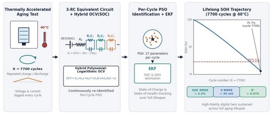
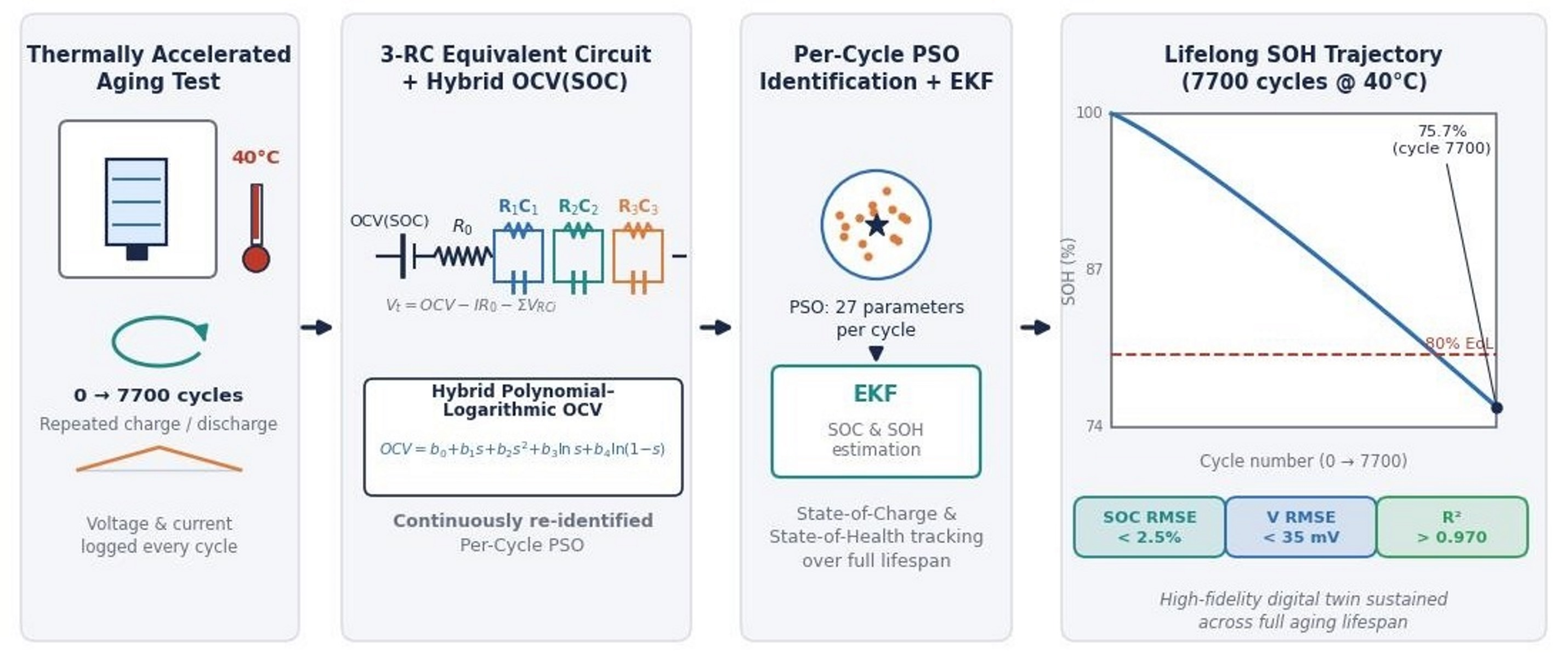
To encourage a wild spread of EVs, accurate SoC and SoH estimation under thermally accelerated aging is critical for advanced BMS systems. This study presents a lifelong degradation analysis of LiBs cells over a 7700 cycle at 40 °C. An adaptive third-order ECM, coupled with a hybrid polynomial–logarithmic OCV formulation, is continuously identified via PSO. The experimental data reveals a distinct degradation profile where the cell crosses the 80% SoH EoL threshold at cycle 5500, steadily declining to a terminal state of 75.7% SoH. Continuous parameter tracking isolates key electrochemical transitions: an initial kinetic stabilization phase is followed by a synchronized thermodynamic OCV realignment near cycle 2000, consistent with increasing LLI. Mid-life aging features a pronounced increase in the time constants, while a late-life degradation is characterized by increasing transport limitations, reflected in the evolution of the slow diffusion-related model parameters, inducing parameter boundary clipping in the slow diffusion branch. Despite these physical non-linearities, the proposed framework maintains high global fidelity throughout the 7700-cycle lifespan, strictly bounding the SoC RMSE below 2.5%, keeping Voltage RMSE under 35 mV, and preserving an R2 above 0.970. Comparative evaluations indicate that the proposed framework achieves a favorable balance between computational efficiency, tracking accuracy, and long-term diagnostic stability.

Graphical Abstract

1. Introduction

In this ever-evolving world, the EV has gained the most interest among recent technologies, due to the necessity for reliable, efficient, and safe energy-storage systems [1,2,3]. Thanks to the reliability, high thermal stability, and long cycle life of LiBs, Lithium became the default technology for EVs [4,5], especially since ambient temperatures and intensive duty cycles are common occurrences [6,7,8]. Even with all the battery advantages, it remains highly sensitive to operating conditions, such as temperature. The degradation phenomena such as SEI layer growth, electrolyte decomposition, and structural changes in electrode materials [9,10,11] are highly susceptible to high temperature, which is the main cause of capacity loss and internal resistance increase, affecting both the SoC and SoH [12,13,14,15].
To estimate SoC and SoH of a battery, BMS depend on mathematical models to infer them [16,17,18]. ECMs are such models used by BMS to represent the non-linearity of a battery for real-time application [19,20]. The accuracy of ECM is dependent on accurate parameter identification, which evolves over time due to aging and is significantly influenced by temperature variations [21,22]. Capturing this parameter evolution is particularly challenging under high-temperature conditions, where nonlinearities and accelerated degradation effects become more pronounced.
In the effort of identifying ECM parameters, a metaheuristic optimization is recommended. Among them, PSO is an optimization capable of solving nonlinear and multi-dimensional problems without finding its gradient. It can also help in tracking ECM parameters throughout the battery aging process, even under severe thermal conditions [23,24]. PSO can additionally be exploited in resolving machine learning and deep learning challenges [25,26,27], such as hyperparameter tuning, neural network training, and model architecture optimization [28,29].
There are various state estimation techniques, one of the most wildly adopted is KF, a recursive algorithm developed for linear dynamic systems, that combines model predictions with real-time measurements to minimize estimation errors [30,31], which provides an accurate system state even with measurement and process noises [32,33]. The KF is exploited in different fields such as aerospace [34], robotics [35], navigation [36], and energy systems [37]. However, LiBs exhibit nonlinear behavior due to the complex electrochemical reactions. To overcome this limitation, the EKF extends the KF framework by linearizing the nonlinear system around the current operating point through first-order Taylor series approximations [38,39]. In BMS, the EKF is applied to estimate critical variables such as the SoC and SoH that cannot be measured directly, and only be indirectly inferred from measurable current, voltage, and temperature.
Prior work has established the combination of an ECM, PSO for parameter identification, and an EKF for state estimation as an effective approach to SoC tracking under fixed or mildly varying operating conditions. What remains comparatively under-explored is the behavior of this pipeline under sustained, elevated-temperature cycling, and whether repeated, cycle-resolved parameter identification can itself serve as a diagnostic signal for state of health. In this work, we exploit the experimental data from Oxford battery dataset [40,41,42], to investigate the ECM-PSO-EKF framework not only for single-cycle SoC estimation, but also to independently re-identify the full parameter set at every aging cycle of a cell aged at 40 °C for approximately 7700 equivalent cycles using Nernst-like OCV polynomial equations [43,44] with hysteresis [45]. This allows us to track the evolution of ohmic resistance, the three RC time constants, and the OCV parameters directly against capacity fade, providing a physically interpretable, model-based alternative to purely data-driven SoH indicators.

2. Materials and Methods

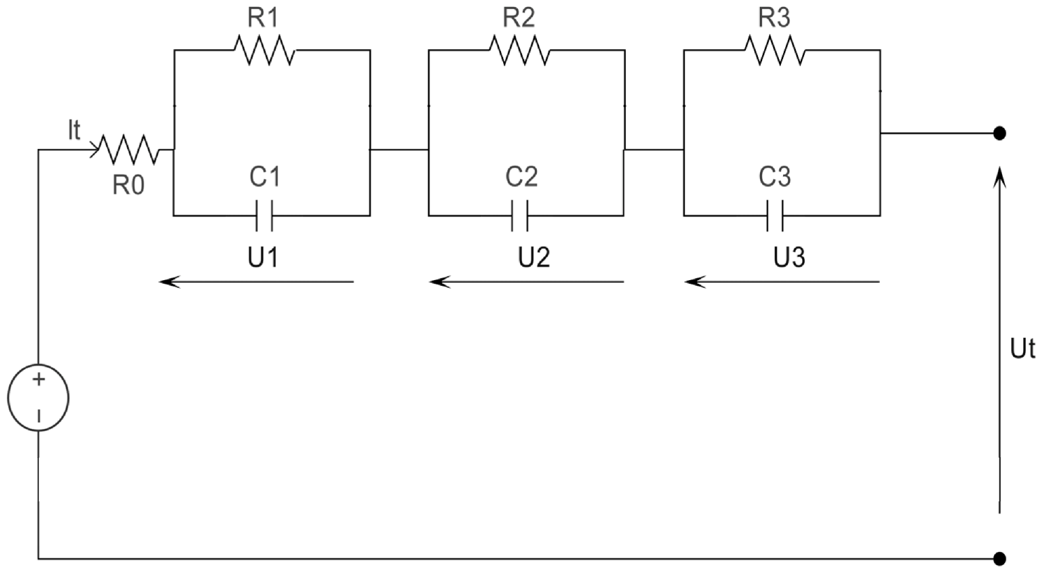
To accurately describe the dynamic behavior of the LiBs, a third-order ECM is adopted (Figure 1). The proposed ECM structure identifies 27 parameters per cycle. While this represents a high-dimensional search space for a stochastic optimizer, the parameters correspond to nine physically distinct RC pairs (fast, mid, and slow relaxation branches, each with separate charge/discharge resistances and shared capacitances) together with the coefficients of the Nernst-like OCV function, rather than an arbitrary parameter count. Physically motivated bounds and expert-initialized particles were used to mitigate the identifiability risk inherent to this dimensionality.
The terminal voltage V t ( t ) is expressed as:
U t ( t ) = U o c v ( S o C ) R 0 I ( t ) U 1 ( t ) U 2 ( t ) U 3 ( t )
where:
I ( t ) is the applied current (positive during discharge).
U 1 , U 2 , U 3 are the voltages across the three RC branches.
The dynamics of each RC branch are governed by:
U ˙ 1 ( t ) = 1 R 1 C 1 U 1 ( t ) + 1 C 1 I ( t )
U ˙ 2 ( t ) = 1 R 2 C 2 U 2 ( t ) + 1 C 2 I ( t )
U ˙ 3 ( t ) = 1 R 3 C 3 U 3 ( t ) + 1 C 3 I ( t )
The State of Charge (SoC) evolution is defined by Coulomb counting:
S o C ˙ ( t ) = I ( t ) Q n o m
where Q n o m is the nominal capacity of the battery.
The behavior of the battery changes between charge and discharge because of hysteresis, so to illustrate the battery as accurately as possible, we use two Nernst-like OCV polynomial equations:
{ U o c v c h ( S o C ) = b 0 c h + b 1 c h · S o C + b 2 c h · SoC 2 + b 3 c h · l n ( S o C ) + b 4 c h · l n ( 1 S o C ) , C h a r g e   ( I < 0 ) U o c v d h ( S o C ) = b 0 d h + b 1 d h · S o C + b 2 d h · SoC 2 + b 3 d h · l n ( S o C ) + b 4 d h · l n ( 1 S o C ) , D i s c h a r g e   ( I > 0 )
To prevent ln(0) explosions during optimization and simulation, the SoC is clipped to S o C s a f e = m a x ( ε , m i n ( 1 ε , S o C ) ) with ε = 10−3.
Discrete equations of ECM can be written as:
U t ( k ) = U O C V ( k ) R 0 I ( k ) U 1 ( k ) U 2 ( k ) U 3 ( k )
U 1 ( k + 1 ) = e T s R 1 C 1   U 1 ( k ) + R 1 ( 1 e T s R 1 C 1 ) I ( k )
U 2 ( k + 1 ) = e T s R 2 C 2   U 2 ( k ) + R 2 ( 1 e T s R 2 C 2 ) I ( k )
U 3 ( k + 1 ) = e T s R 3 C 3   U 3 ( k ) + R 3 ( 1 e T s R 3 C 3 ) I ( k )
S o C ( k + 1 ) = S o C ( k ) T s Q n I ( k )
PSO is a population-based metaheuristic optimization algorithm. It is widely used to solve complex optimization problems where classical methods struggle (nonlinear, nonconvex, or noisy systems). PSO maintains a population of N candidate solutions (“particles”) in the parameter space, each with a position x i ( t ) and velocity v i ( t ) . At each iteration, particles are attracted toward their personal best position ( p b e s t i ) and the global best position ( g b e s t ):
v i ( t + 1 ) = w · v i ( t ) + c 1 r 1 ( p b e s t i x i ( t ) ) + c 2 r 2 ( g b e s t x i ( t ) )
where r 1 , r 2 are numbers between 0 and 1.
x i ( t + 1 ) = x i ( t ) + v i ( t + 1 )
The choice between exploration ( w m a x ) and exploitation ( w m i n ) is important, to realize that an adaptive inertia equation is necessary:
w ( t ) = w m a x ( w m a x w m i n ) · t t m a x
To prevent runaway particle, a velocity and position clamping can be written as:
v m a x = 0.15 · ( u b l b )
v i clip ( v i , v m a x , + v m a x )
x i clip ( x i , l b , u b )
The personal best update and global best update are made following:
p i ( t + 1 ) = { x i ( t + 1 ) if   J ( x i ( t + 1 ) ) < J ( p i ( t ) ) p i ( t ) otherwise
g ( t + 1 ) = a r g m i n p i ( t + 1 ) J ( p i ( t + 1 ) )
For each particle (parameter set), the model is simulated forward in time on both charge and discharge profiles, producing simulated voltages V s i m c h ( k ) and V s i m d h ( k ) . The base error is the weighted RMSE:
e c h ( k ) = V m e a s c h ( k ) V s i m c h ( k )
e d h ( k ) = V m e a s d h ( k ) V s i m d h ( k )
R M S E c h = k w c h ( k ) · e c h ( k ) 2 k w c h ( k )
R M S E d h = k w d h ( k ) · e d h ( k ) 2 k w d h ( k )
EKF is a nonlinear version of the KF widely used for SoC and SoH estimation in batteries because the battery model is nonlinear. To estimate SoC for a third-order ECM, Equations (8)–(11) are used to find the following state-space equation:
[ S O C ( k + 1 ) U 1 ( k + 1 ) U 2 ( k + 1 ) U 3 ( k + 1 ) ] = [ 1 0 0 0 0 e Δ T τ 1 0 0 0 0 e Δ T τ 2 0 0 0 0 e Δ T τ 3 ] [ S O C ( k ) U 1 ( k ) U 2 ( k ) U 3 ( k ) ] + [ Δ T 3600 Q r a t e d ( 1 e Δ T τ 1 ) R 1 ( 1 e Δ T τ 2 ) R 2 ( 1 e Δ T τ 3 ) R 3 ] I ( k ) + w ( k )
with X = [ S O C ( k ) U 1 ( k ) U 2 ( k ) U 3 ( k ) ] is the State Vector, A k = [ 1 0 0 0 0 e Δ T τ 1 0 0 0 0 e Δ T τ 2 0 0 0 0 e Δ T τ 3 ] is State Matrix, B k = [ Δ T 3600 Q r a t e d ( 1 e Δ T τ 1 ) R 1 ( 1 e Δ T τ 2 ) R 2 ( 1 e Δ T τ 3 ) R 3 ] is System Control Vector, and w(k) is the System Process Noise where its covariance is Q.
The measurement equation from Equation (7) is as follows:
U t , k = U O C V ( k ) I ( k ) R 0 U 1 ( k ) U 2 ( k ) U 3 ( k ) + v ( k )
where v ( k ) represents Measurement Noise and R its covariance.
EKFs require a Jacobian Matrix to function because the cell is a non-linear system, especially the Nernst-like OCV polynomial equations:
H k = d x d h = [ d S O C d O C V 1 1 1 ]
From Equation (6):
d S O C d O C V = b 1 + 2 b 2 + b 3 ( S O C + ε ) b 4 ( 1 S O C + ε )
EKF also requires equations to predict the State Vector, covariance matrix and terminal voltage:
X ^ k = A k x ^ k 1 + B k I k
P ^ k = A k P k 1 A k T + Q
U ^ t , k = O C V ( S O C ^ k ) U ^ 1 , k U ^ 2 , k U ^ 3 , k R 0 I k
To determine Kalman Gain K k , we have to first determine innovation covariance Sk:
S k = H k · P ^ k · H k T + R
K k = P ^ k · H k T · S k 1
Finally, the update to EKF is realized though:
X k = X ^ k + K k ( U t , k U ^ t , k )
P k = ( I K k · H k ) · P ^ k
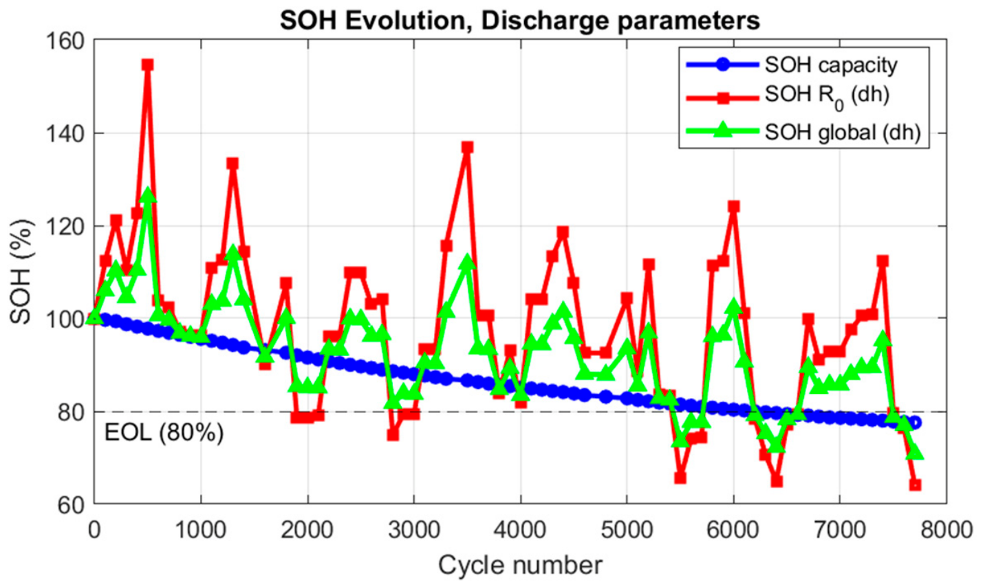
We can determine capacity, R 0 , and the global health ( S o H ) as the following equations:
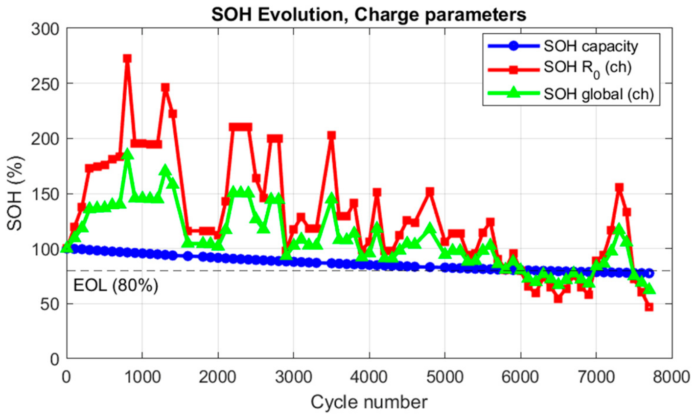
S o H c a p a c i t y = Q c y c l e ( n ) Q c y c l e ( 0 ) · 100 %
S o H R 0 = R 0 c y c l e ( 0 ) R 0 c y c l e ( n ) · 100 %
S o H g l o b a l = S o H c a p a c i t y + S O H R 0 2
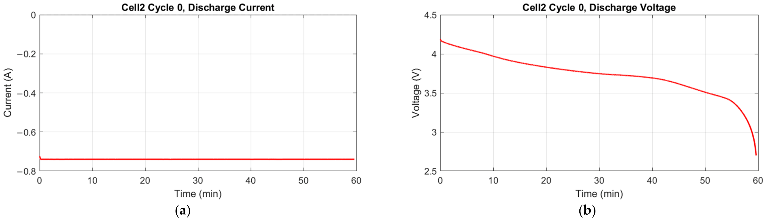
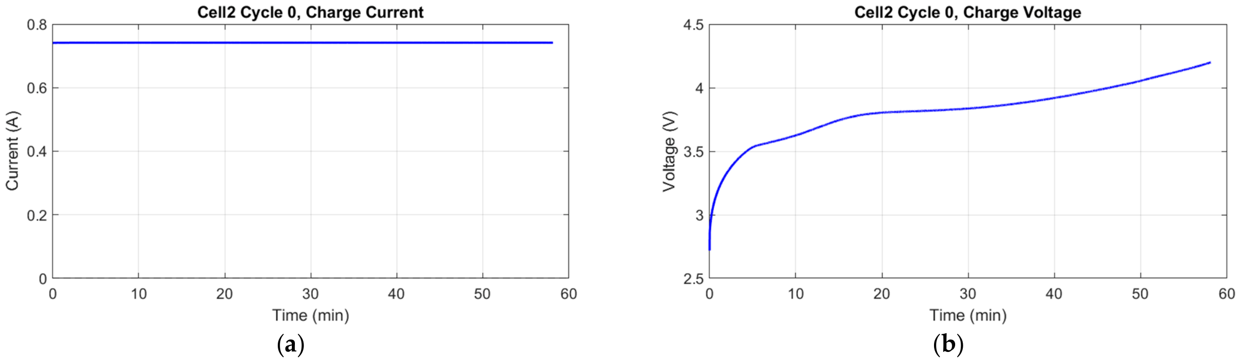
To study the evolution (from cycle 0 to 7700) of the parameters of a cell with PSO optimization, we use Oxford Data, where the LCO/NCO cell Kokam CO LTD, SLPB533459H4 has a capacity 740 mAh, and applies continuous 1-C current (740 mA) for both charge and discharge at 40 °C. Figure 2 and Figure 3 illustrate the voltage and current used in those both phases at the first cycle (cycle 0):
The parameters deployed in PSO optimization need bounds to limit the area of search for cell parameters. Table 1 illustrates these limits:
The key parameters for PSO optimization, such as the number of particles used in multiple optimization cycles, are shown in Table 2.

3. Results

In this section, we will showcase the evolution of battery parameters from cycle 0 to 7700 including resistances, capacitance, time constants, coefficients for Nernst-like OCV polynomial (b0, b1, b2, b3, and b4), capacity, and SoC and SoH.

3.1. Resistances Evolution Analysis

3.1.1. Resistance R0

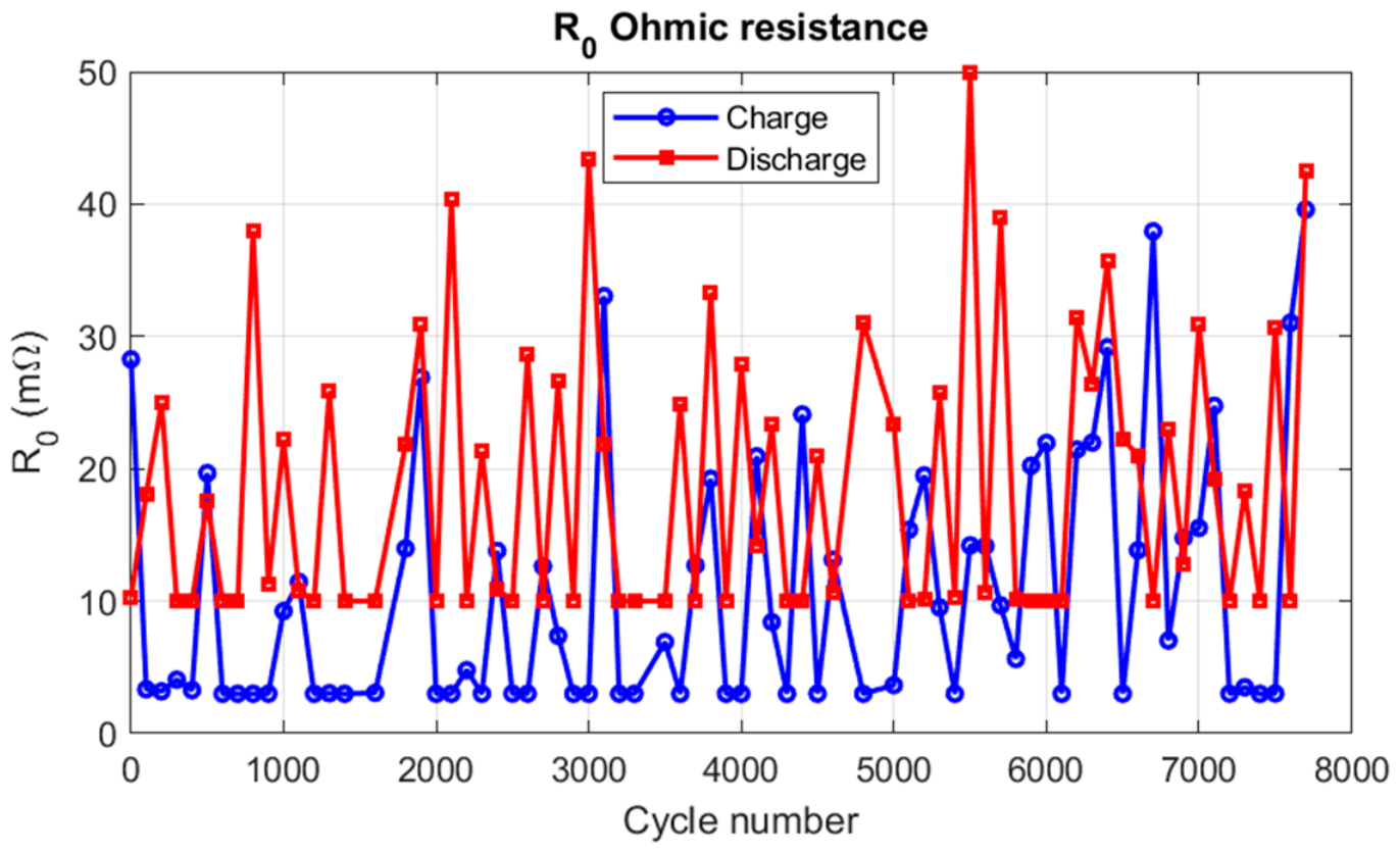
Figure 4 represents the evolution of R0 through 7700 cycles of battery life, in both charge (blue) and discharge (red) curves. The two curves share a consistent limit value around 3 and 10 mΩ. This denotes the nominal, uncompromised ohmic resistance of the cell under high operating temperatures and specific SoC throughout the aging process.
There is a clear divergence between the two operating modes. The discharge resistance experiences vastly more frequent and higher magnitude spikes than the charge resistance across the entire lifespan.
While the first 5000 cycles show a highly stable baseline for charging and mostly flat lining near 3 mΩ, the final 2000 cycles show a distinct behavioral shift. The charge resistance baseline breaks upward, and both curves exhibit massive, concurrent spikes reaching peaks between 40 and 50 mΩ.
The ohmic resistance R0 shows the most consistent monotonic increase across all cycles. This trend is consistent with progressive SEI layer growth and gradual electrolyte conductivity loss, both of which are accelerated under sustained elevated-temperature operation.

3.1.2. Resistance R1

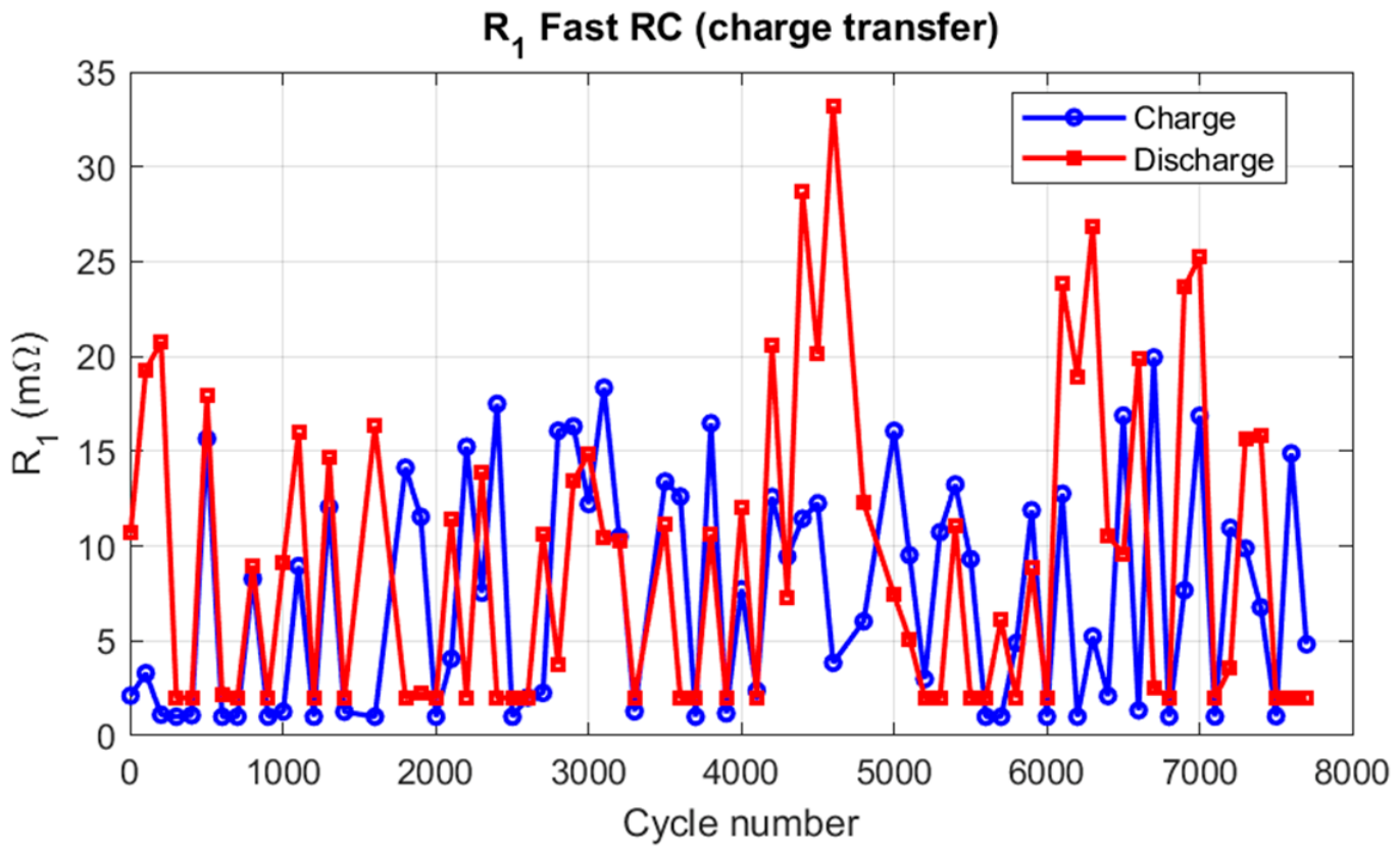
Similar to the R0 plot, Figure 5 shows resistance R1 as a very rigid, recurring lower limit at approximately 1 and 2 mΩ for both charge and discharge lines across the entire lifespan.
Up until cycle 4000, the charge and discharge curves share a highly overlapping operational envelope, generally fluctuating between 1 mΩ and 20 mΩ. However, between cycles 4000 and 5000, the discharge resistance experiences a massive, sustained surge, peaking at over 33 mΩ, while charging remains largely bound to 15 mΩ.
In the final 2000 cycles, the charge transfer resistance becomes highly erratic for both operating modes. Unlike the mid-life phase where discharge dominated, the charge and discharge curves show massive, alternating spikes that frequently trace each other’s amplitudes up to 20 and 27 mΩ.

3.1.3. Resistance R2

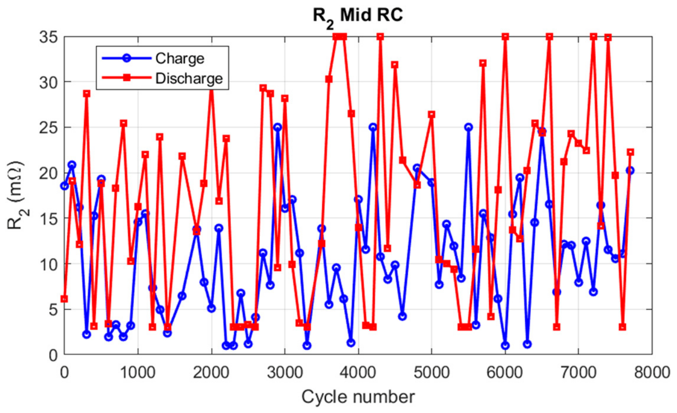
Across nearly the entire lifespan, the discharge resistance acts as an upper envelope to the charge resistance. While the charge curve spends significant time oscillating in the lower 0–15 mΩ zone, the discharge curve frequently shoots upward, maintaining a much higher mean resistance. At different cycles such as 3600, 3900, 4300, 6000, 6600, 7100, and 7400, the discharge resistance hits the upper limit of 35 mΩ. We can conclude that R2 behavior is highly erratic and that the resistance varies from the lower to the upper limit from one cycle to another (Figure 6).
The R2 resistance also increases with aging, though less monotonically than R0. This is consistent with charge-transfer resistance growth from active material loss and increased diffusion resistance from electrode microstructural changes.

3.1.4. Resistance R3

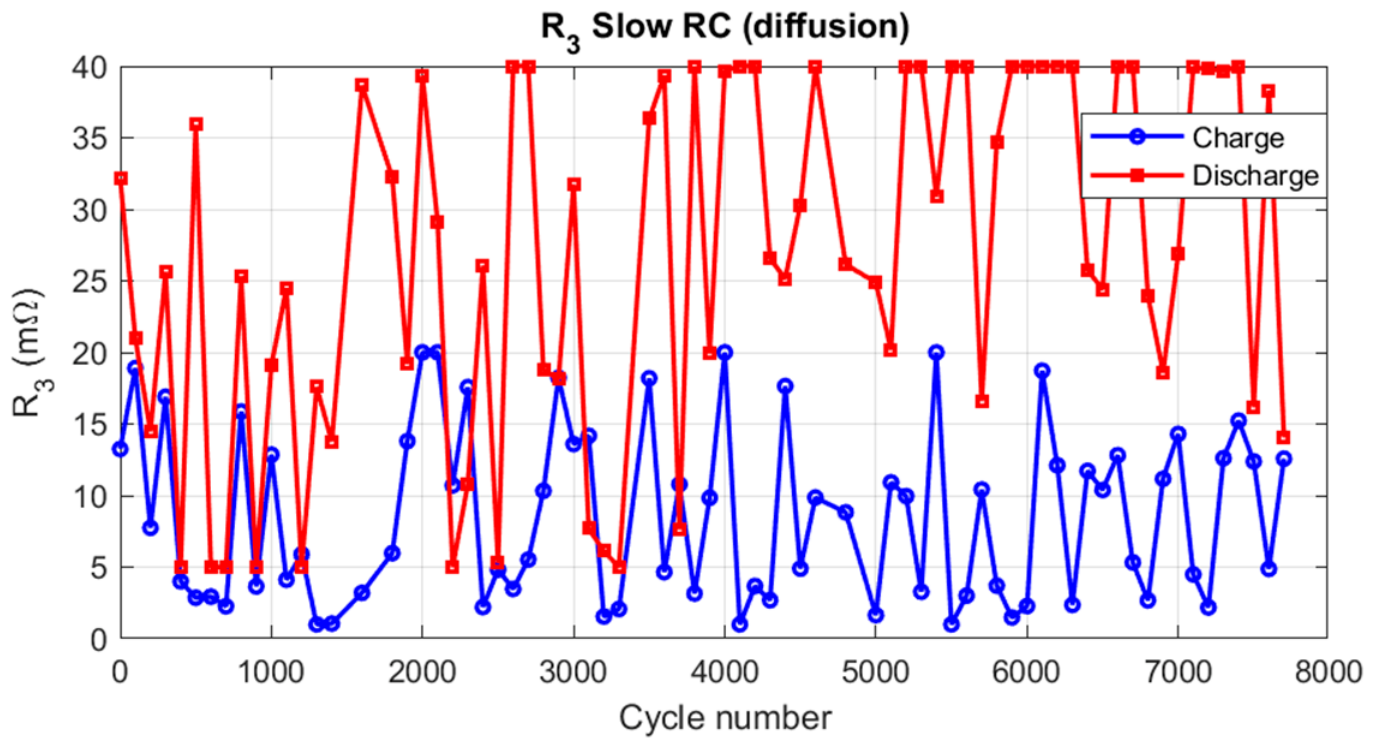
In Figure 7, we notice the biggest difference between charge and discharge resistance, where charge resistance varies between 1 and 20 mΩ through all the cycles. But the discharge resistance has two main sections, the first one between 0 and 3200 cycles, where the resistance drops to a lower bound at 5 mΩ a few times, and the second section from 3200 to 7700, where the resistance remains mostly at the upper limit of 40 mΩ.
Despite the intense degradation of the cell, the lower bound of the charging diffusion resistance remains remarkably unaffected, continuously dipping back to 1–3 mΩ even up to cycle 7700. The corresponding increase in resistance R3 in the slow time constant τ3 = R3C3 indicates measurable slowing of solid-state diffusion over the cell’s aging trajectory.

3.2. Capacitances and Time Constants Evolution Analysis

3.2.1. Capacitance C1 and Time Constant τ1

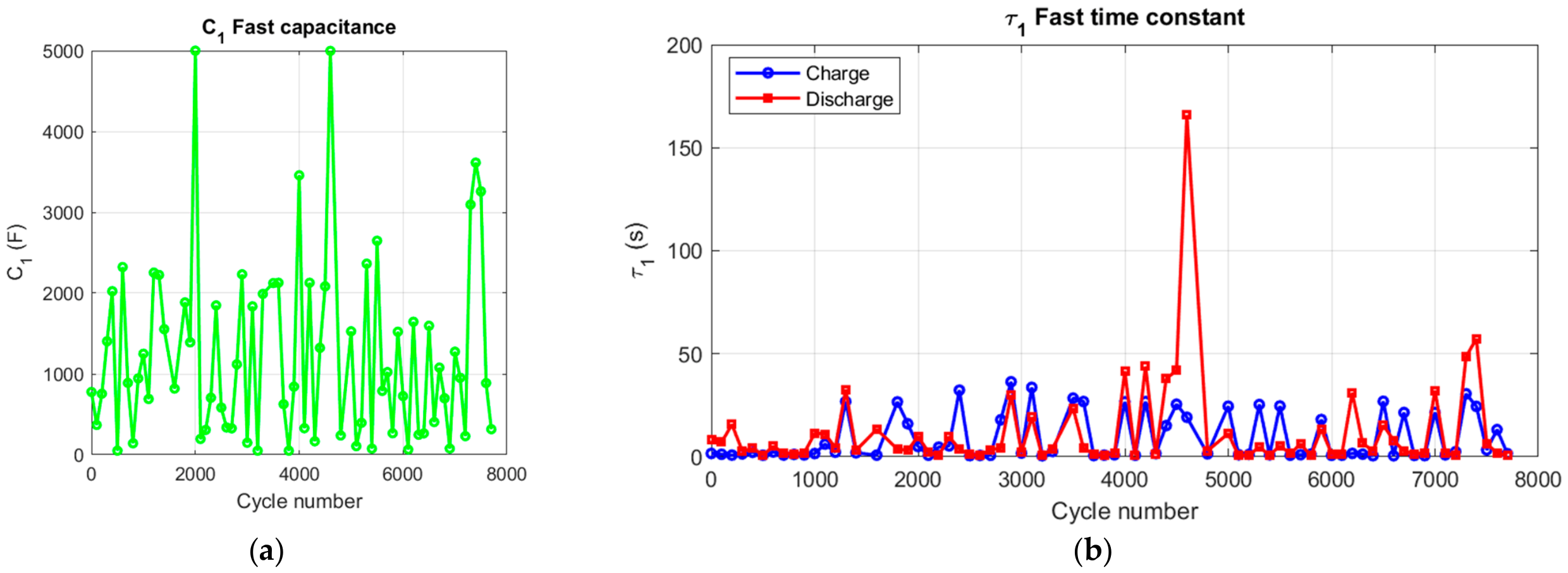
In Figure 8a, the capacitance C1 is maintained at a relatively stable baseline; C1 swings violently between nearly 0 F and over 3000 F from cycle to cycle across the battery’s entire lifecycle. There is no clear single long-term upward or downward trend line. But C1 hits the upper limit (5000 F) at around 2000 and 4600 cycles.
In Figure 8b, the time constant remains tightly compressed below 30 s for both charge and discharge throughout 7700 cycles. But at 4600 cycles, only the discharge time constant surges to 165 s, yet the charge time constant during this exact same time remains safely under 25 s.

3.2.2. Capacitance C2 and Time Constant τ2

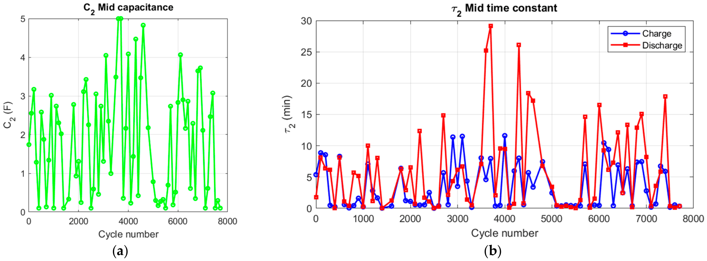
Unlike the fast capacitance C1, which peaked at thousands of Farads, in Figure 9a, C2 operates on a much lower physical scale, capped tightly at an upper bound of exactly 5 F. While highly unstable, there is a visible macro-trend from cycles 2500 to 4800 where the capacitance baseline and peak frequency migrate upward, hovering consistently between 2 F and 5 F before dropping down sharply post-cycle to 5000.
For the first 2500 cycles, as shown in Figure 9b, the charge and discharge time constants track each other remarkably closely, staying beneath 10 min. However, past cycle 2500, the discharge curves begin spiking dramatically higher than the charge transients. The absolute maximum of the discharge curve occurs near cycle 3700, exploding upward to a prolonged relaxation phase of 29 min.

3.2.3. Capacitance C3 and Time Constant τ3

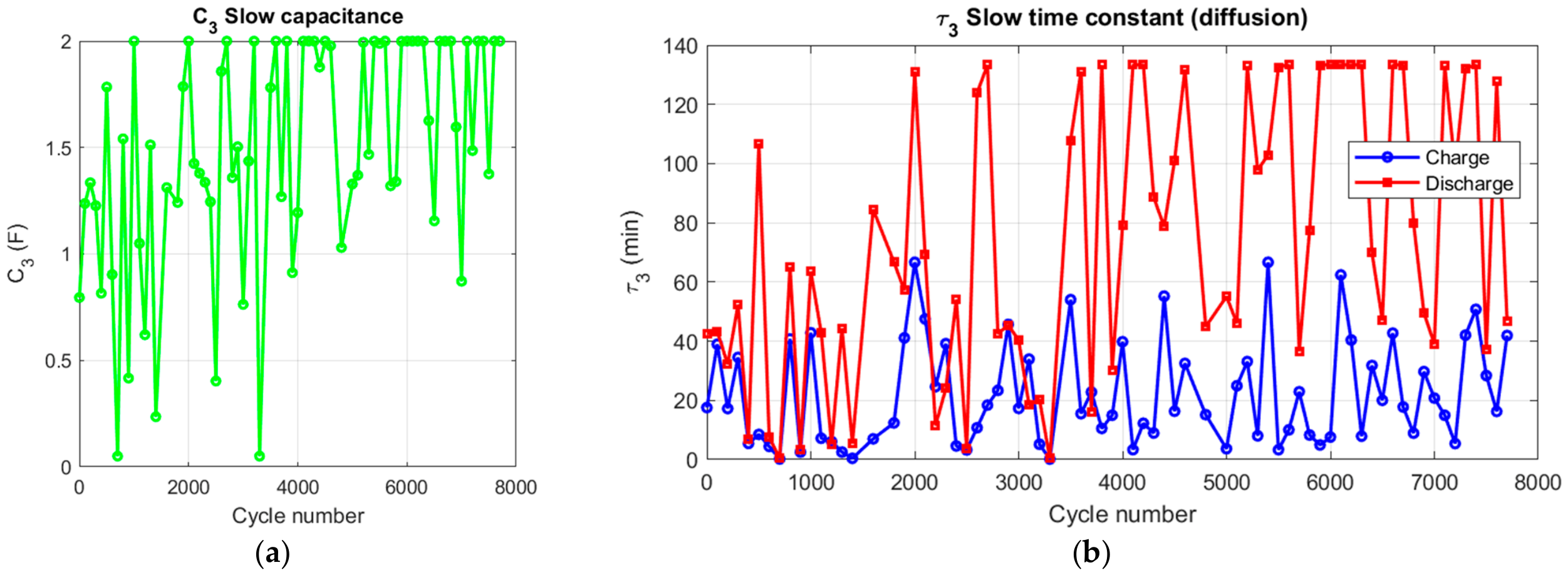
C3 operates on a very small numerical scale, strictly constrained to an upper limit of exactly 2 F. In the first 3000 cycles, the capacitance baseline fluctuates wildly between 0 F and 2 F. However, as the cell progresses past cycle 4000, the data becomes heavily concentrated near the top ceiling, frequently pinning itself to the 2 F maximum up to the end of testing (Figure 10a).
The gap between time constant charge and discharge is massive. The charge τ3 fluctuates between 0 and 60 min through the entire aging of the cell, the discharge time constant oscillates in the same time in much higher values, where it varies between 80 and 133.3 min. This fluctuation hits the upper limit more often at late cell life (after 5700 cycles) as shown in Figure 10b.

3.3. OCV Coefficients and Curves Evolution Analysis

3.3.1. OCV Coefficient b0

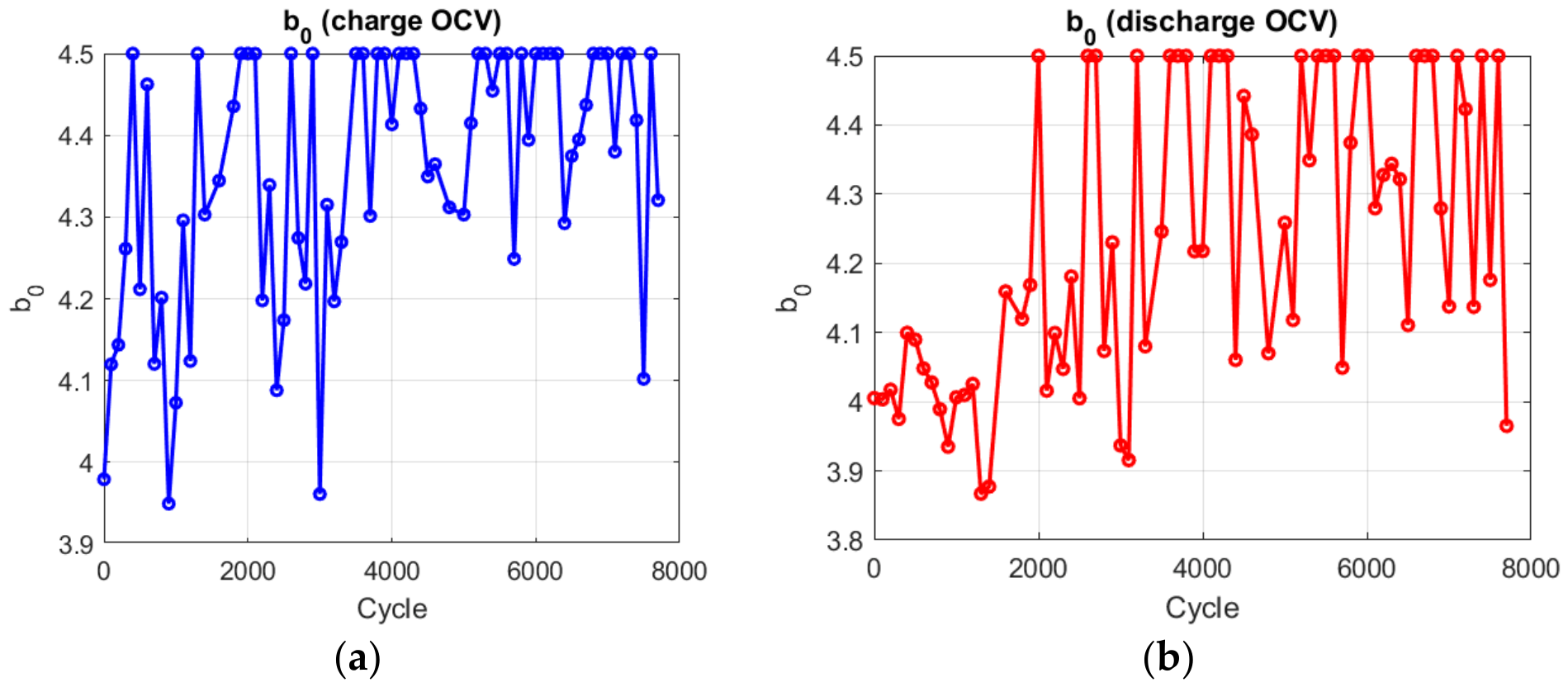
Figure 11 tracks the evolution parameter b0 of Nernst-like OCV polynomial equations and both charge and discharge of the ECM model. Between cycles 0 and 3500, b0 charge behaves unsteadily, dipping down to 3.95 a few times, before stabilizing to 4.5 past the 3500 cycles.
Unlike the charge plot, the discharge baseline shows a distinct, progressive evolution. During the first 1500 cycles, b0 remains relatively low, fluctuating between 3.85 and 4.1. Between cycles 1500 and 2000, the parameter experiences a dramatic upward shift, permanently changing its operational baseline. Past cycle 2000, it mirrors the charge curve by frequently clipping against the 4.5 upper optimization ceiling.

3.3.2. OCV Coefficient b1

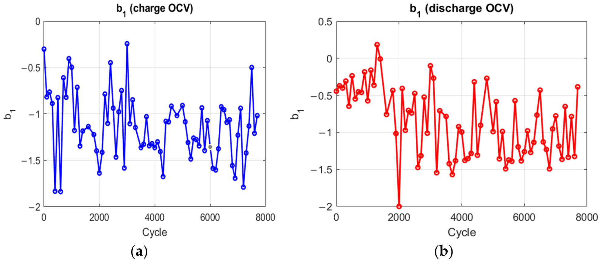
From cycle 0, b1 exhibits aggressive a high-frequency oscillations spanning almost the entire optimization window (from −0.2 down to −1.85). Unlike the previous parameters, b1 during charge never hits a flat, saturated ceiling or floor boundary, indicating that the search bounds for this specific parameter were sufficiently wide (Figure 12a).
In the first 1500 cycles, the discharge slope coefficient remains tightly bound and relatively flat, hovering in a shallow region between −0.2 and −0.6. At cycle 2000, the discharge curve plunges violently to its absolute minimum value of −2.0. Following that major drop, the discharge curve completely loses its early-life stability. It transitions into a highly erratic, wider-band oscillation pattern (mostly between −0.5 and −1.5) that closely mirrors the behavior of the charge curve for the remainder cycles (Figure 12b).

3.3.3. OCV Coefficient b2

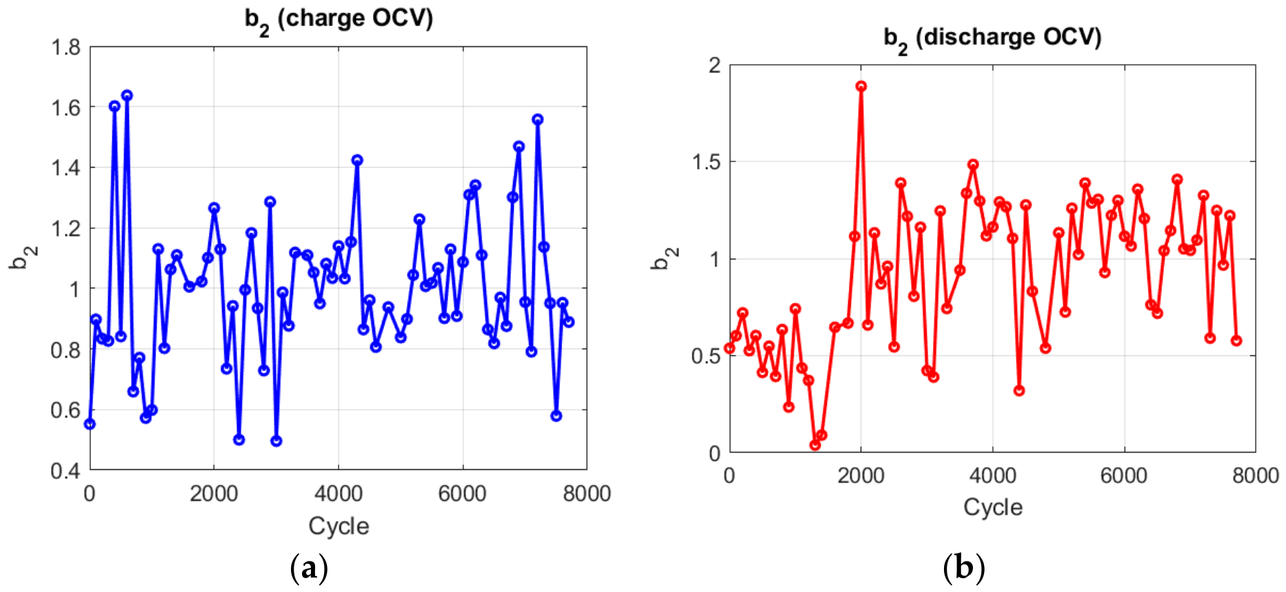
From Figure 13a, we notice that the parameter b2 fluctuates between 0.5 and 1.65 intensely without being clipped by the bounds of the optimization to match active charging dynamics of the cell.
In Figure 13b, the discharge parameter b2 has completely different behavior, where in first cycles (up to cycle 2000), the parameter remains between 0.05 and 0.75, then it shoots upward to a 1.9 value, followed by oscillation between 0.6 and 1.5 through the remaining cycles.

3.3.4. OCV Coefficient b3

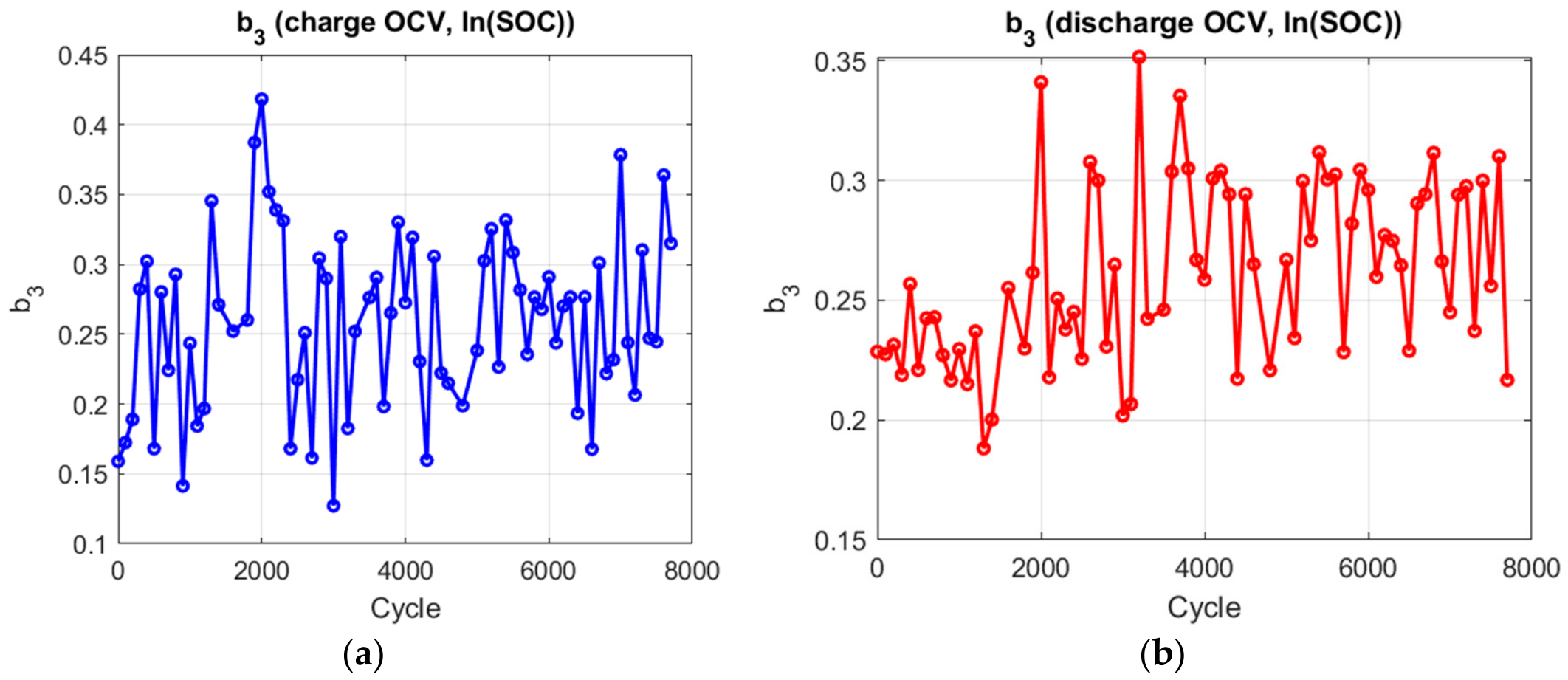
In Figure 14a, the first 2000 cycles show that the charge b3 has a high frequency variation between 0.16 and 0.35 before reaching 0.42 at cycle 2000; afterward, the charge parameter never returns to a low value of 0.16—it remains at slightly higher values (between 0.2 and 0.38) for the following cycles.
Figure 14b showcases the behavior of b3 discharge in 7700 cycles; the discharge has the same demeanor as the charge parameter but at different values, it starts at 0.23, then fluctuate moderately in the 2000 cycles between 0.18 and 0.26. At cycle 2000, b3 discharge increases to 0.34 and it oscillates mostly between 0.22 and 0.34 with a peak at cycle 3600.

3.3.5. OCV Coefficient b4

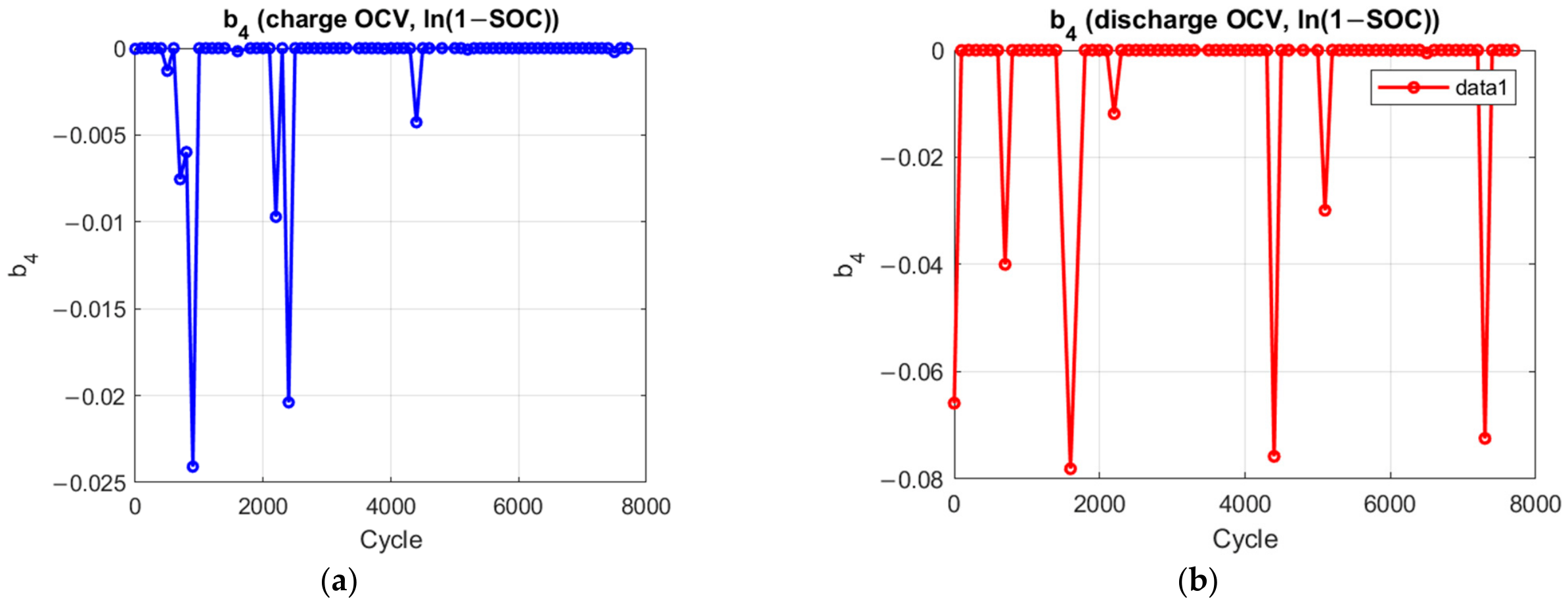
In Figure 15a, the b4 charge plot exhibits intense, high frequency throughout the entire 7700-cycle span. Despite the volatility, the macro-baseline remains relatively flat, consistently bouncing within a narrow corridor between −0.010 and −0.035 with no clear upward or downward step changes.
In the first 1500 cycles, the b4 discharge plot stays very tightly bound in a shallow region close to zero (between −0.005 and −0.015). At the 2000-cycle threshold, the parameter undergoes a dramatic downward plunge, dropping to −0.045. Post cycle 2000, the discharge parameter completely loses its initial tight containment. The baseline permanently shifts downward, matching the wide, volatile envelope of the charge curve for the remaining lifecycle (Figure 15b).

3.3.6. OCV Curves

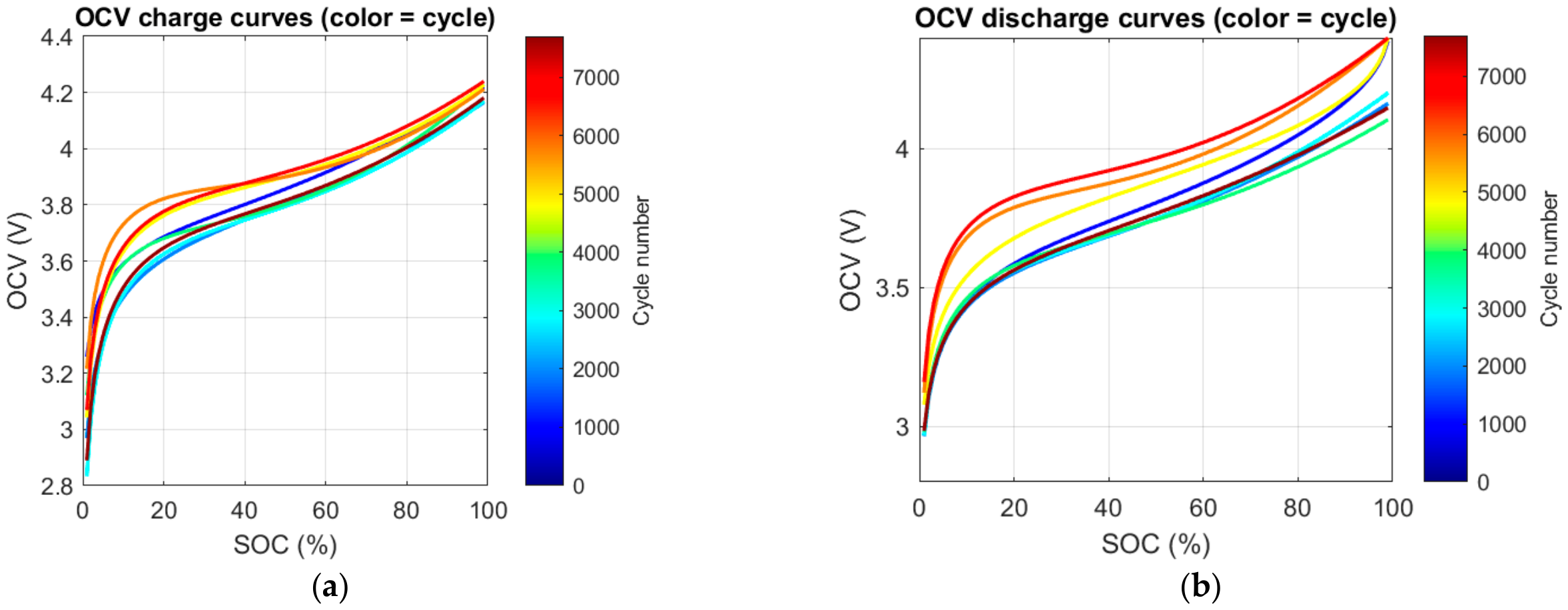
In Figure 16a, all the OCV charge curves, regardless of the cycle age (from cycle 1 to cycle 7700), successfully converge at the same upper boundary of 4.2 V at 100% SoC. But between the 10% and 60% SoC window, the curves noticeably shift upward as the cell ages. At a fixed low SoC (around 20%), an aged cell (red/orange lines) exhibits a higher open-circuit voltage than a fresh cell (blue/purple lines). The curvature at the lower boundary (0% to 10% SoC) becomes increasingly steep and sharp as cycling progresses past 4500 cycles.
In Figure 16b, the fresh-cell OCV discharge curves drop smoothly toward the 3.0 V cutoff at 0% SoC, while the aged curves (cycles 6000–7700) exhibit a massive, precipitous cliff. The voltage profile between 0% and 20% SoC completely collapses downward in late life. The smooth curve deforms into a sharp, rigid “L shape” right before depletion.
At the nominal voltage plateau around 50% SoC, the curves start to be separated as the cell ages across all 7700 cycles, showing very significant vertical drift.
The gradual evolution of the OCV-SOC relationship may reflect changes in lithium inventory and electrode stoichiometry during aging. As cyclable lithium is consumed through parasitic side reactions such as SEI growth, the equilibrium potential profile shifts, requiring progressive adaptation of the OCV model coefficients.

3.4. State of Charge and Capacity Evolution Analysis

3.4.1. SoC and RMSE Early Life

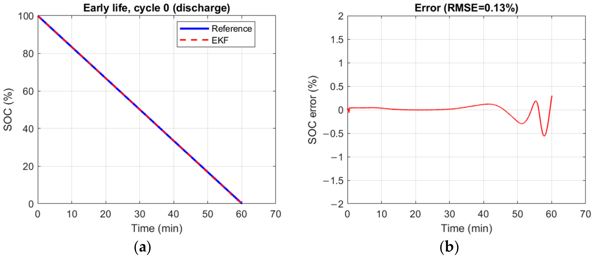
Figure 17a represents a cell undergoing an Urban Artemis driving profile, with 1C discharge current stepping down from 100% SoC to 0% SoC over roughly 60 min. At the early life of a cell, both the EKF-estimated SoC and the reference are indistinguishable across the entire dynamic profile. As for Figure 17b, the RMSE error remains tightly compressed beneath a maximum peak of 0.2%. For the vast majority of the test, the error hovers well below 0.05%. The highest value is achieved upon reaching 10% SoC, where the error starts fluctuating.

3.4.2. SoC and RMSE Mid-Life

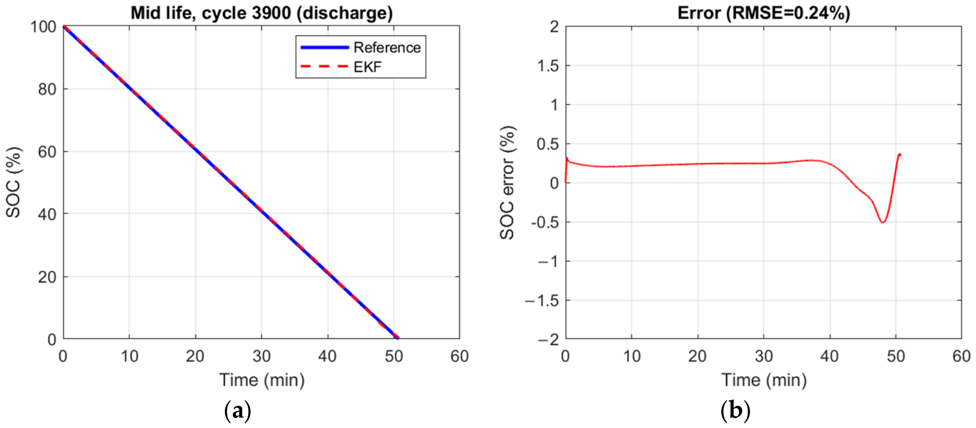
Unlike the cycle 0 test which took roughly 60 min to deplete the cell, the cycle 3900 test profile terminates much sooner, ending at approximately 50 min. Even though the cell is heavily aged, the estimated SoC curve still tracks the experimental measurements exceptionally well during the discharge phase (Figure 18a). Throughout the nominal operating window, tracking error stays almost constant as long as SoC is higher than 36% at around 0.5%. After that, the error goes higher than 0.7%, then at around 17% starts going down to −0.8% before climbing back up to 0.2% (Figure 18b).

3.4.3. SoC and RMSE End-Life

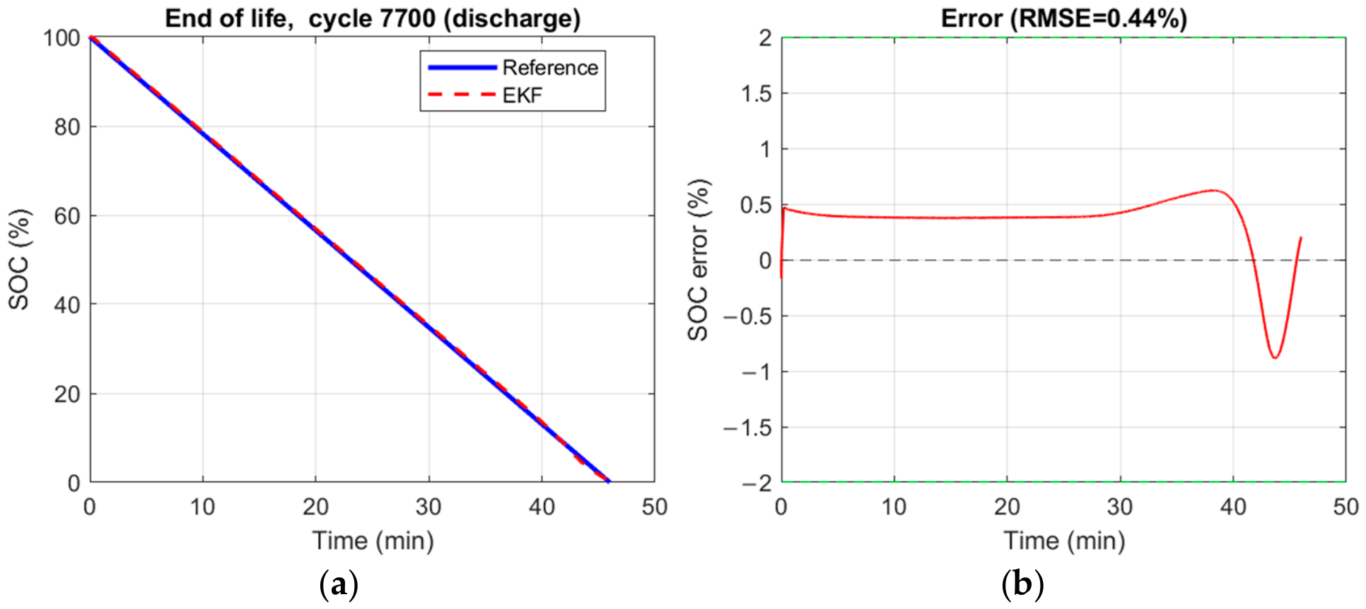
In this end-of-life cycle, the cell only lasted 46 min, a little less than the 50 min of 3900 of the mid-of-life. Even when the error goes from 0.24% to 0.44%, as in Figure 19b, we noticed that the tracking of SoC is still functioning, which means that the error is still in tolerable bounds (Figure 19a).

3.4.4. Cell Capacity

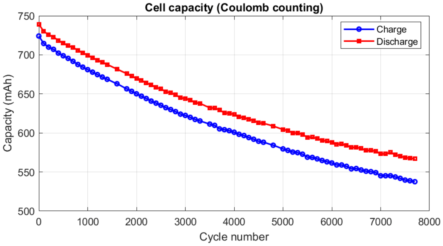
The capacity curve for both charge and discharge follow the same behavior, so we will focus on the effective energy which is the discharge curve (Figure 20). The capacity curve does not follow a linear path. Instead, it exhibits a three-stage battery degradation trajectory under high thermal stress:
Stage 1 (Cycles 0 to 1500): A highly stable, linear, and slow aging phase. The capacity decreases marginally from 740 mAh down to approximately 680 mAh.
Stage 2 (Cycles 1500 to 5500): At cycle 1500, we notice an acceleration in the capacity fading. The capacity curve knows a change in behavior; a non-linearity is observed and by the end, the capacity drops from 680 mAh to 600 mAh.
Stage 3 (Cycles 5500 to 7700): Beyond this point, the capacity fade plunges exponentially, collapsing down to an ultimate EoL value of 580 mAh at cycle 7700.
Capacity fade proceeds from 100% to approximately 75.7% SoH over the 7700 cycles analyzed. The degradation trajectory remains predominantly smooth and monotonic, without the pronounced knee commonly associated with accelerated degradation regimes such as severe lithium plating or rapid active-material loss. The observed trend is more consistent with progressive SEI growth and gradual lithium inventory loss under sustained elevated-temperature operation. Although the rate of capacity loss increases slightly at later life stages, no distinct degradation knee is observed before dataset termination.

3.5. Errors Evolution Analysis

3.5.1. RMSE Error

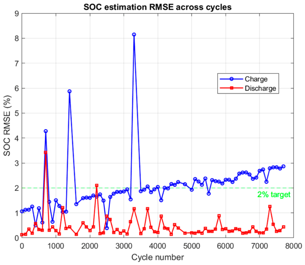
While validation curves from Figure 17, Figure 18 and Figure 19 showed detailed, single-cycle snapshots (cycles 0, 3900, and 7700), Figure 21 shows the continuous metric performance across all 7700 cycles. For the charge curve, RMSE remains extraordinarily low and stable, strictly confined below 2% and maintaining with a few peaks 4.2%, 6% and 8.1% at 800, 1500, and 3300 cycles respectively, mostly likely due to a wrong choice in PSO optimization parameter quickly corrected in the first 5500 cycles. Exactly at the 5500-cycle threshold, the error experiences an abrupt change in slope and breaks upward, climbing steadily past 2% and peaking at almost 3% at the late stage of life. As for the discharge curve, it stays mostly under 1% with a few peaks to 4.2% at the 800 cycle and 2.2% at the 2200 cycle.

3.5.2. R2 Error

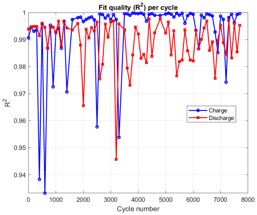
While RMSE quantifies absolute error in volts or percentage points, R2 measure the relative strength of the model’s explanatory power. The most notable feature of Figure 22 is that both charge and discharge R2 values remain consistently high throughout the battery lifetime, generally exceeding 0.98 and frequently approaching 1.
At the beginning of life, the battery exhibits very low internal resistance and rapid electrochemical dynamics due to the elevated operating temperature of 40 °C. Between approximately 1500 and 5500 cycles, despite these ongoing degradation processes, the model continues to maintain strong predictive capability. The ability of the PSO algorithm to continuously adapt the RC parameters allows the equivalent circuit model to accurately track the evolving electrochemical behavior. Nevertheless, even during these fluctuations, the majority of R2 values remain above 0.97, confirming the robustness of the model. Beyond approximately 5500 cycles, the scatter of both curves increases noticeably. Despite this increased complexity, the R2 values remain remarkably high. Most values continue to exceed 0.98, while the lowest observed values remain above approximately 0.94–0.95. This indicates that the proposed model retains strong predictive capability even near EOL.

3.6. State of Heath Evolution Analysis

3.6.1. Charge SoH

The estimated SoH curve (red) tracks the experimental SoH curve (blue) with near-perfect overlap across the entire 7700-cycle aging history. The two lines in Figure 23 are virtually indistinguishable through all macro-phases of degradation. In the early life of a cell (from cycle 0 to 1500), we notice a slow linear health degradation phase, with SoH dipping slightly from 100% down to 96%. As for the middle of life of the cell (cycles 1500 to 5500), there is an intermediate linear degradation phase, where the battery health declines at a faster rate from 96% down to the standard industrial EOL of 80% SoH. Beyond cycle 5500, the cell degrades below the 80% threshold and the SoH drops to almost 47% SoH.

3.6.2. Discharge SoH

In Figure 24, we observe exceptional tracking of the experimental discharge SoH (blue line) by the estimated discharge SoH (red line), where the estimated SoH follows the experimental one with zero delay across all the cycles. For first 1500 cycles, the SoH changes steadily from 100% to 96%. After the 1500 cycle, the degradation of SoH is accelerated and drops below 80% around 5500 cycles. From then onward, the SoH reaches the value of 75.7% by the EOL of the cell.

3.7. Parameters Sensitivity

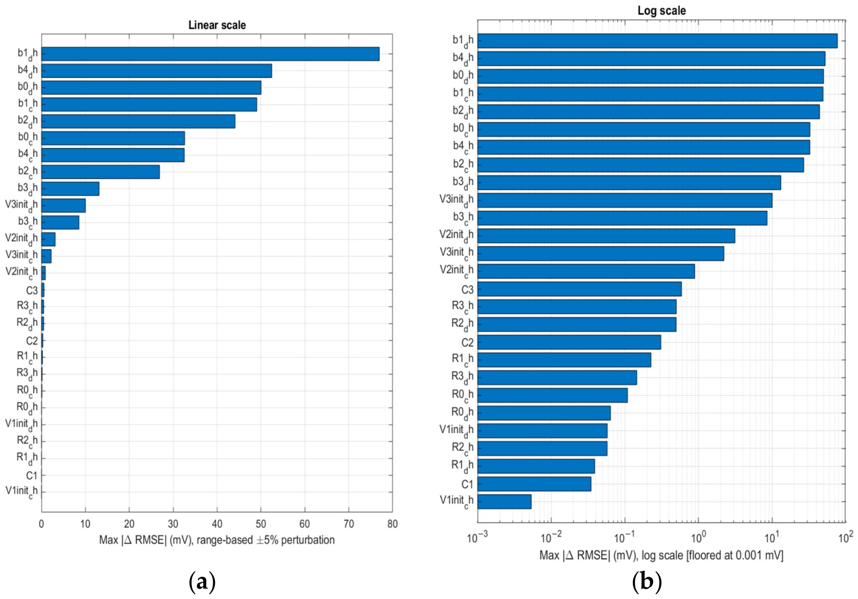
A perturbation-based sensitivity analysis was performed, in which each of the 27 parameters was individually shifted by ±5% of its permitted search range around the PSO-optimized value, and the resulting change in voltage RMSE was recorded. The open-circuit voltage (OCV) coefficients were found to be the most strongly identified parameters, with perturbations producing RMSE changes of 8–77 mV, consistent with the OCV term dominating the terminal voltage over the full State of Charge trajectory. In contrast, the ohmic and RC-branch parameters (R0, R1–R3, C1–C3) produced RMSE changes below 1 mV under equivalent perturbations. We attribute this to the near-constant-current nature of the characterization segments used for parameter identification, under which the RC branches are only weakly excited; their voltage contribution approaches a near-constant offset that is partially absorbed by the OCV baseline term during fitting. This indicates that while the OCV parameterization is tightly constrained by the available data, the resistance and capacitance parameters including R0, which was investigated as a resistance-based aging indicator, are comparatively less identifiable from this excitation profile, and their quantitative values are less strongly constrained than the OCV coefficients and their cycle-to-cycle fluctuations should therefore be interpreted with greater caution than the corresponding long-term aging trends, which does not depend on this identification step (Figure 25).

4. Discussion

The present study is based exclusively on cells aged under a constant 40 °C environment, as provided by the Oxford Battery Degradation Dataset. While this isolates the effect of sustained elevated-temperature aging on parameter evolution, it does not allow us to verify the generalization of the identified parameter trends or the SoC/SoH estimation accuracy across a wider temperature range. Consequently, the reported parameter trajectories should be interpreted as specific to the investigated thermal condition rather than universally representative of LiB aging behavior. Nevertheless, the proposed PSO-EKF framework itself is independent of the specific temperature used during aging and could be applied to cells characterized under alternative thermal conditions, provided that temperature-specific parameter identification is performed.
R0 plot illustrates the evolution of the ohmic resistance R0, throughout the aging process at 40 °C. During the first 5500 cycles, R0 remains relatively low and stable at 3–5 mΩ, indicating efficient ionic conduction and favorable electrolyte transport conditions promoted by the elevated operating temperature. The low resistance values suggest that the electrolyte and current collector interfaces remain largely intact during the early and middle stages of battery life. As cycles progress beyond 5500, a pronounced increase in R0 is observed. The sharp spikes represent local minima where the algorithm overcompensated R0 to fit a highly non-linear voltage curve. This transition marks the onset of severe aging phenomena, including electrolyte depletion, loss of interfacial contact, and degradation of electronic conduction pathways. Repeated volume expansion and contraction of the electrodes contribute to particle cracking and delamination, increasing the effective ohmic resistance can be potentially associated with continuous operation at 40 °C where the electrolyte evaporates or breaks down via chemical reduction much faster than it would at a standard room temperature (25 °C). The sharp fluctuations observed near end-of-life indicate increasing heterogeneity within the cell, where localized degradation mechanisms dominate the overall electrical response. The divergence between charge and discharge values further highlights the dynamic nature of R0, demonstrating that resistance is influenced not only by SoH but also by operating direction and electrochemical conditions, because during discharge, lithium ions are stripped from the anode and forced through the electrolyte to intercalate into the cathode. As the cell empties, the electrolyte near the electrode surfaces can face localized concentration polarization (ion depletion). This temporarily starves the conduction path, physically increasing the ohmic bulk resistance. But during charge, the phase kinetics and internal mechanical pressures within the jelly-roll/pouch stack often facilitate slightly better contact mechanics and lower initial impedance.
The resistance R1 plot reflects the kinetics of electrochemical reactions occurring at the electrode–electrolyte interfaces. Throughout the early stages of cycling, R1 remains relatively low, indicating efficient lithium–ion exchange across the interfaces, proving the kinetic benefit of an elevated testing temperature of 40 °C, where the optimized ion mobility and interfacial kinetics result in highly stable, low-resistance baselines. A noticeable increase in discharge R1 appears around cycle 4500, suggesting significant growth and restructuring of the SEI. As the SEI layer thickens, lithium ions encounter a larger activation barrier during extraction, resulting in higher resistance during discharge than during charging. Beyond 5500 cycles, high-amplitude synchronized chaotic behavior mirrors the trend seen in R0, confirming that the cell has passed its degradation in both charge and discharge resistances exhibit highly unstable behavior. This instability is attributed to continuous particle cracking and repeated formation of fresh SEI layers on newly exposed electrode surfaces most likely due to the high temperature. Consequently, the available reaction area changes continuously, leading to strong cycle-to-cycle variability in the estimated R1 values. These results indicate that R1 serves as an effective indicator of interfacial degradation and electrochemical aging.
The intermediate-frequency resistance R2 and low-frequency diffusion resistance R 3  provide insight into transport limitations within the electrode structure. The frequent saturation of R2 at its upper optimization bound set to 35 mΩ indicates that the actual resistance exceeded the predefined search limits during several aging stages. This behavior highlights the increasing difficulty of lithium–ion transport through the growing SEI/CEI layers. Elevated temperature accelerates the formation and restructuring of these interfacial films, producing significant transport bottlenecks, particularly during discharge. Similarly, R3 exhibits progressive growth with aging and eventually reaches its optimization boundary of 40 mΩ. Unlike R2, which mainly reflects interfacial transport limitations, R3 is associated with solid-state diffusion within the active materials. The sustained increase in R3 suggests severe structural degradation, including particle cracking, loss of active material, and disruption of lithium diffusion pathways. The persistent saturation of both parameters during late-life operation is consistent with the transport phenomena as the battery approaches EoL.
The capacitance C1 exhibits significant variability throughout cycling, reflecting the well-known difficulty of identifying capacitance values using optimization-based techniques. Since capacitance primarily affects short-duration transients, limited high-frequency excitation in the experimental current profile (continuous 1C) has reduced parameter identifiability, where the algorithm is constantly searching across the bounds to minimize error, frequently hitting the 5000 F boundary limit. Despite the fluctuations in C1, the associated time constant τ1 provides clearer physical interpretation. A pronounced peak occurs around cycle 4500, coinciding with the maximum observed R1. Under the influence of 40 °C thermal stress, the SEI/CEI reached a temporary point of extreme instability or structural restructuring. The combination of a high kinetic barrier (R1) and a highly polarized double-layer capacitive effect (C1) temporarily slowed down the battery’s voltage recovery dynamics during discharge, stretching its fast relaxation time from a few seconds to nearly three minutes.
The intermediate time constant τ2 reaches its highest values between approximately 3700 cycles, where both R2 and C2 hit their high-limit bounds (0.035 Ω and 50,000 F respectively). τ2 hitting nearly 29 min shows the optimizer stretches the time constant out to nearly half an hour to minimize fitting errors. Between 2500 and 4000 cycles, we noticed an accelerated SEI/CEI growth, which increases the time required for interfacial charge redistribution following current perturbations. Following this peak, both C2 and τ2 decrease substantially, indicating that surface-film growth has reached a relatively stable state. At this stage, degradation mechanisms shift away from interfacial processes toward bulk structural deterioration.
The diffusion-related branch exhibits the strongest degradation effects. Simultaneous saturation of R3, C3, and τ3 during late life suggests that the model approaches its identification limits (0.04 Ω, 200,000 F, and 133.3 min respectively) when attempting to reproduce extremely slow diffusion processes. Continuous cycling at 40 °C promotes structural disorder within the cathode crystal lattice and causes micro-cracking due to repeated phase transitions. During discharge, when lithium is being forced back into the host material, these structural defects act as microscopic energy traps and act as dominant kinetic bottleneck forcing the macroscopic voltage relaxation tail to drag out for over two hours. During early-to-mid-life aging (0–4000 cycles), Bulk Structural Degradation is still manageable by the model, then the late-life degradation past 6000 cycles induces severe LAM and lattice damage. The battery develops relaxation dynamics so slow (exceeding 133 min) that they completely outgrow standard metaheuristic search boundaries during discharge.
The evolution of the polynomial–logarithmic OCV coefficients reveals a major thermodynamic transition occurring between approximately 1500 and 2000 cycles.
Initially, all coefficients remain relatively stable, indicating preservation of the original OCV-SoC relationship. However, a synchronized shift occurs near cycle 2000:
  • b0 increases significantly.
  • b1 becomes more negative.
  • b2 and b3 reach their maximum values.
  • b4 exhibits a sharp decrease.
This collective behavior suggests a fundamental modification of the battery’s equilibrium voltage characteristics. The observed changes are consistent with LLI, electrode stoichiometric imbalance, and structural transformations within the active materials. The increasing importance of logarithmic and inverse OCV terms indicates that voltage behavior near low SoC becomes progressively more nonlinear as aging advances. Consequently, the OCV model requires stronger correction terms to accurately represent the evolving electrochemical equilibrium.
The reconstructed OCV curves provide direct evidence of the thermodynamic changes identified through the parameter analysis. During early life, both charge and discharge OCV curves exhibit smooth profiles with well-defined voltage plateaus. As aging progresses, the low-SoC region becomes increasingly distorted, eventually developing a steep voltage collapse near the depletion boundary. This deformation is characteristic of severe lithium inventory loss and active material degradation. The pronounced low-SoC voltage drop indicates increasing difficulty in sustaining electrochemical reactions as available lithium and active reaction sites decrease. The OCV evolution therefore may indicate that aging affects not only kinetic parameters but also the fundamental equilibrium behavior of the cell.
The PSO-identified 3RC model shows an excellent performance throughout the battery lifetime. At beginning-of-life, voltage tracking errors remain below 20 mV, while SOC estimation errors remain below 1.25%, confirming accurate representation of the battery dynamics. At cycle 3900, despite significant aging, the model maintains voltage errors below 10 mV for most operating conditions. Larger deviations appear only near low-SoC regions where strong nonlinearities dominate the voltage response. At cycle 7700, voltage and SoC estimation errors increase to approximately 122 mV and 7.5%, respectively. These deviations coincide with severe structural degradation and increased internal heterogeneity, conditions that challenge the assumptions of lumped-parameter equivalent circuit models. Nevertheless, lifecycle-average performance remains highly satisfactory, with SOC RMSE generally below 2.5%, voltage RMSE below 35 mV, and R2 values consistently above 0.97. These results demonstrate the robustness of the proposed PSO-based identification framework even under severe thermal aging conditions.
The capacity degradation profile reveals three distinct aging stages:
  • Stage I (0–1500 cycles): Capacity decreases slowly, indicating relatively stable operation with limited degradation.
  • Stage II (1500–5500 cycles): A noticeable increase in degradation rate occurs following the thermodynamic transition identified in the OCV parameters. Accelerated SEI growth and continuous lithium consumption become the dominant aging mechanisms.
  • Stage III (>5500 cycles): The cell reaches the degradation knee and experiences rapid capacity collapse. This stage is characterized by severe electrolyte depletion, active material loss, and diffusion limitations.
The SoH trajectory closely follows this three-stage behavior, confirming the strong relationship between internal parameter evolution and macroscopic battery health. The combined analysis reveals a clear degradation sequence under continuous cycling at 40 °C:
  • Early Life (0–1500 cycles): Stable electrochemical behavior with low resistance and minimal capacity loss.
  • Thermodynamic Transition (1500–2000 cycles): Onset of significant lithium inventory loss and OCV restructuring.
  • Interfacial Degradation (2000–5500 cycles): Accelerated SEI/CEI growth produces increasing charge-transfer and transport limitations.
  • Bulk Structural Failure (>5500 cycles): Active material loss, particle cracking, electrolyte depletion, and diffusion starvation dominate battery behavior.
This progression suggests that elevated-temperature operation initially improves electrochemical kinetics but ultimately accelerates the degradation mechanisms responsible for capacity fade, resistance growth, and end-of-life failure.
While standard combinations of ECMs and optimization algorithms are widely reported in the literature, existing studies rarely evaluate higher-order networks over extended, multi-thousand-cycle aging horizons. Most reported ECM-based estimation frameworks are evaluated over substantially shorter aging horizons than the present study and rarely investigate parameter evolution across the complete degradation trajectory. The primary novelty of this work lies in the lifelong tracking capability of the proposed adaptive 3-RC framework coupled with a hybrid polynomial-logarithmic OCV formulation.
To demonstrate the competitive advantage and long-term tracking robustness of the proposed methodology, our results are benchmarked against recent State-of-the-Art frameworks, including IEKF w/SA-PSO [46], WMISAEKF [47], VFFRLS + EKF-LSBoost [48], a 2nd-order RC comparison study [49], and Bayesian Optimization vs. PSO [50]. As summarized in Table 3, the proposed framework maintains stable tracking across an extensive 7700 cycle horizon at 40 °C, accurately mapping internal parameter evolution down to a terminal state of 75.7% SoH without filter divergence or numerical instability.
Unlike the compared studies, which primarily focus on SoC estimation accuracy, the proposed framework additionally analyzes the evolution of the identified ECM parameters over the full aging trajectory and investigates their suitability as physically interpretable SoH indicators. It should be noted that the studies summarized in Table 3 were conducted using different cells, operating conditions, datasets, and validation protocols. Consequently, the comparison is intended to provide qualitative positioning relative to the State-of-the-Art rather than a strict quantitative ranking.
To characterize the run-to-run variability of the PSO identification procedure, two complementary tests were performed. First, the algorithm was repeated N = 15 times with independent random seeds on a representative cycle: discharge voltage RMSE ranged from 15.2 to 37.1 mV (mean 21.4 ± 5.6 mV), and the identified ohmic resistance R0 ranged from 0.010 to 0.046 Ω. Second, to confirm this variability is not specific to a single cycle, the identification was independently repeated three times for every cycle in the dataset (73 datasets (7700 cycles) × 3 = 219 runs total), retaining the lowest-cost result per cycle (“best-of-three”). Table 4 reports the resulting error statistics.
Computational cost per cycle (three repetitions combined) averaged 99.7 ± 17.5 s across all 73 cycles (equivalent to approximately 33.2 s per individual PSO run). The single outlier (221 s, the first cycle processed) is attributable to MATLAB R2024a (MathWorks Inc., Natick, MA, USA) just-in-time compilation overhead on first execution rather than a genuine per-cycle cost difference; excluding it, computational time was highly consistent across the remaining 72 cycles (98.0 ± 10.0 s per cycle, range 82–115 s). This indicates that, aside from a one-time startup cost, the computational burden of per-cycle PSO identification is stable and predictable across the cell’s aging trajectory, which is relevant to the offline/edge-deployment feasibility.
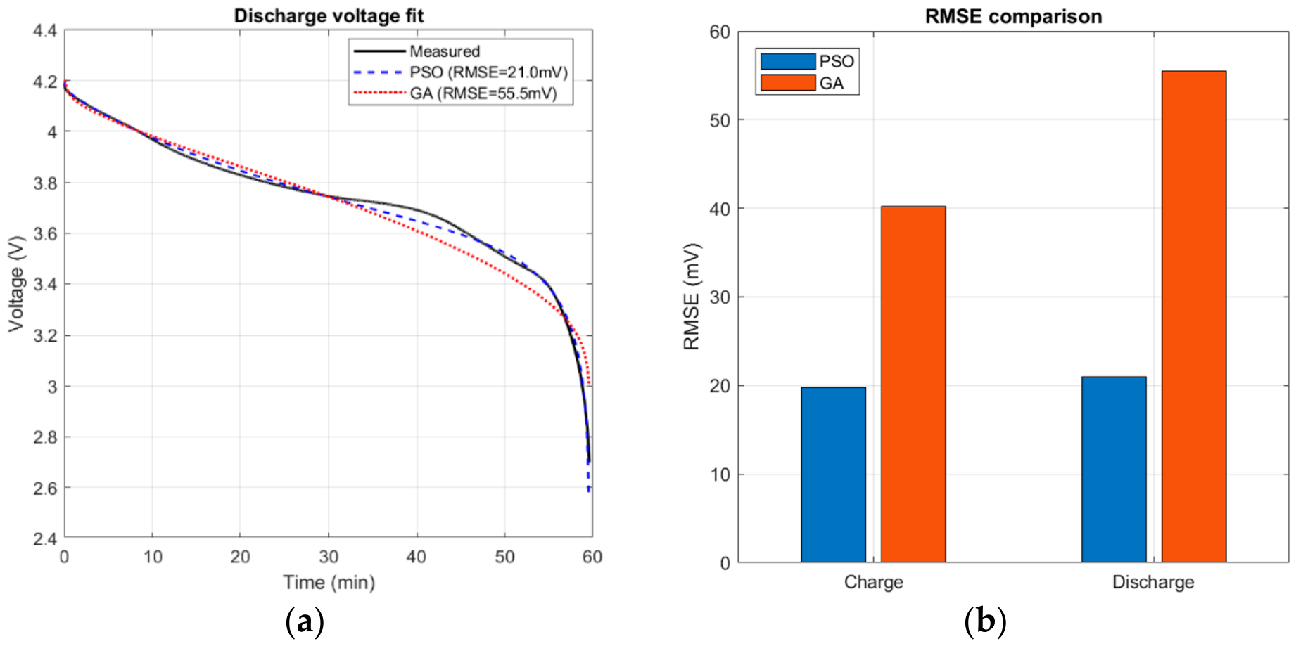
To verify the advantage of PSO over a classic alternative optimizer, the identical 27-parameter identification problem (same cost function, bounds, and cycle-0 data) was solved using a genetic algorithm (GA) with a matched computational budget (population 200 × 300 generations ≈ 60,000 cost evaluations, versus PSO’s 200 particles × 300 iterations = 60,000 evaluations). At comparable wall-clock time (39.2 s for PSO vs. 40.1 s for GA), PSO achieved substantially lower error (discharge RMSE 21.0 mV, R2 = 0.993) than GA (discharge RMSE 55.5 mV, R2 = 0.948), a 2.6-fold reduction in RMSE. This supports the use of PSO over GA for this high-dimensional, continuous parameter identification problem under an equal evaluation budget. These results indicate that, for the present high-dimensional nonlinear identification problem, PSO provides a better balance between convergence quality and computational cost than a conventional GA under an equivalent evaluation budget (Figure 26).
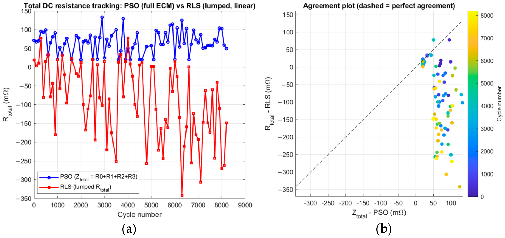
As a further baseline representative of recursive parameter-estimation methods commonly used in battery-management systems, recursive least squares (RLS) was applied to track a lumped total DC resistance (R0 + R1 + R2 + R3), using each cycle’s PSO-identified OCV curve as a known input and assuming the RC branches reach steady state within the 60 min characterization segment, the standard simplifying assumption required to make RLS applicable to this problem. The dashed diagonal line in Figure 27 represents the line of perfect agreement (y = x), where both methods would produce identical Z total values. Points lying on this line indicate complete agreement, whereas the distance from the line reflects the magnitude of the discrepancy between the two methods. The validity of this comparison was limited for the present dataset: the slowest (diffusion) time constant identified by PSO frequently exceeds 100 min, well beyond the segment duration, so the corresponding RC branch voltage does not settle within the available data window. Under this violated assumption, RLS resistance estimates differed substantially from the values obtained by the full nonlinear PSO identification (mean absolute discrepancy 156 mΩ against resistances on the order of 50–100 mΩ) and occasionally produced negative resistance estimates, indicating violation of the assumptions required by the simplified RLS formulation. These results suggest that simplified recursive linear estimators become difficult to apply when the dominant diffusion dynamics evolve on timescales longer than the available characterization segment. Under such conditions, the full nonlinear multi-RC identification performed by PSO is better able to capture the coupled resistance–capacitance dynamics without requiring steady-state assumptions.
To study the cost of the framework PSO-EKF in multicycles, we start with analysis of PSO in a single cycle where the benchmark indicates that a single cost function evaluation requires approximately 0.90 ms, corresponding to about 709 kFLOPs (0.71 MFLOP). This cost is mainly associated with simulating the equivalent circuit model over the entire charge and discharge datasets, which contain 3492 and 3578 samples, respectively. Therefore, more than 99% of the computational effort originates from the battery model simulation itself, while the optimization constraints have a negligible impact on the overall cost. This is consistent with the fact that computational complexity scales primarily with the number of measurement points used during parameter identification.
OCV coefficients (b0–b4) are strongly identified (8–77 mV RMSE change under perturbation), while resistance/capacitance parameters (R0–R3, C1–C3) are comparatively weakly identified (<1 mV change), because the characterization segments are near-constant-current, so the RC branches are only weakly excited and their contribution is partly absorbed into the OCV baseline term during fitting.
Although the identification problem is high-dimensional, convergence difficulties were mitigated through physically constrained parameter bounds and expert-informed particle initialization. Furthermore, repeated optimization experiments showed that the voltage-fitting performance remained consistent across independent runs, indicating that the PSO algorithm can reliably locate solutions with similar objective-function values despite the dimensionality of the search space. The newly added sensitivity analysis further clarifies which parameters are strongly constrained by the available data and which are comparatively weakly identifiable.
Temporal distribution: Contrary to the intuitive expectation that clipping would become more frequent near end-of-life, no meaningful correlation was found between clipping frequency and cycle number for the most-affected parameters (|r| ≤ 0.33 in all cases). Clipping is a structural property of the identification problem present throughout the cell’s life, not an aging-specific artifact.
Diffusion branch (R3, C3): Comparing the diffusion time constant τ3 = R3C3 against each cycle’s actual characterization segment duration, mean τ3 (75.7 min) exceeds the mean segment duration (51.4 min); in 64.4% of cycles τ3 exceeds the available window entirely, directly explaining the observed clipping (47.9% of cycles have R3 or C3 at their upper bound) as a consequence of the characterization protocol. Because the diffusion branch is not fully observable within the available characterization window, multiple combinations of R3 and C3 can produce nearly indistinguishable voltage trajectories. Consequently, clipping of these parameters introduces a bias toward saturated diffusion time constants and may artificially limit the apparent growth of the diffusion-related resistance components. Therefore, individual per-cycle values of R3 and C3 should not be interpreted as precise physical measurements; rather, their long-term trends provide a qualitative indication of degradation progression.
OCV coefficient b4: This coefficient clips at its upper bound (0) in 92–100% of cycles. To distinguish a genuine optimum from an overly restrictive bound, the identification was re-run on six cycles spanning the cell’s full life with the b4 upper bound relaxed from 0 to 0.3. In all six cycles, b4 converged back near zero regardless of the available range (mean b4,ch = 0.006, mean b4,dh = −0.019), confirming a genuine, consistent optimum rather than a bound artifact. The negligible change in RMSE after relaxing the bound further indicates that the clipping of b4 does not introduce a meaningful estimation bias and is instead a consequence of the optimum OCV representation naturally lying near b4 = 0.
For a single aging cycle, the PSO configuration employs 200 particles and 300 iterations resulting in: 200 × 300 = 60 , 000 cost-function evaluations.
The total execution time is estimated at 54 s, corresponding to approximately 42.56 GFLOPs. This result indicates that although a single model evaluation is computationally inexpensive, the repeated evaluations required by the swarm optimization process accumulate into a significant computational load. This behavior is characteristic of population-based metaheuristic algorithms, which sacrifice computational efficiency in exchange for robust global search capabilities and reduced sensitivity to local minima. The computational demand is nevertheless acceptable because parameter identification is typically performed offline and does not require real-time execution.
As for multicycles, when the optimization is repeated for all 7700 aging cycles, the total computational effort increases to 70 min (1.17 h) of execution time and 3.32 TFLOPs of computations. This substantial increase is expected because the optimization process is independently executed for each cycle to track the evolution of battery parameters during aging. The resulting computational cost reflects the extensive search performed by PSO to accurately identify the ECM parameters throughout the battery lifetime. Although the total processing time appears large, it remains practical for research and offline battery characterization studies where accuracy is prioritized over execution speed.
The EKF benchmark suggests significantly lower computational requirements for a complete discharge profile containing 3578 samples, where the execution time is 4.5 ms and the computational cost is 0.72 MFLOPs. Compared with the PSO optimization stage, the EKF requires approximately:
42.56 × 10 9 0.72 × 10 6 59,000
times fewer floating-point operations.
This enormous difference indicates that the EKF is highly suitable for real-time implementation within a BMS. The low computational burden results from the recursive nature of the EKF, which updates the state estimate sequentially at each sample rather than performing iterative global optimization.
Applying the EKF over all aging cycles requires only 0.7 s and 111.63 MFLOPs. This shows that SoC estimation can be performed efficiently even when analyzing large battery-aging datasets. The computational cost remains negligible compared with the parameter identification stage. The results therefore support the common strategy of:
  • Performing PSO parameter identification offline.
  • Using the identified parameters within an EKF for online SoC estimation.
This architecture effectively combines high modeling accuracy with real-time feasibility.
The computational analysis suggests a clear separation between the offline and online stages of the proposed methodology. The PSO-based parameter identification represents the dominant computational burden, requiring approximately 3.32 TFLOPs for the complete aging dataset. However, this cost remains acceptable because parameter identification is performed offline and benefits greatly from parallel processing where we can reduce the time from 70 to 7 min for 14 core CPU. In contrast, the EKF exhibits extremely low computational requirements, requiring only 4.5 ms per cycle and less than 1 s for the entire dataset. These results confirm the suitability of the proposed PSO-EKF framework for practical battery management applications, where computationally intensive optimization can be conducted offline while maintaining real-time SoC estimation capability through the EKF. The analysis further highlights the scalability of the approach and its potential for deployment in embedded BMS and large-scale battery aging studies.
A critical consideration for the proposed adaptive updating strategy is its viability on embedded BMS platforms constrained by sampling frequency and computational latency. Executing the full 27-parameter PSO identification directly at the sampling rate typically used in battery management systems (10–100 Hz) would exceed the computational resources of most automotive-grade microcontrollers. Consequently, the proposed framework is intended for a dual-time-scale architecture. The EKF performs real-time SoC estimation using the most recently identified parameter set, while the computationally intensive PSO optimization is executed at a much slower rate using accumulated historical data. Such updates could be performed offline during charging periods, scheduled maintenance events, or through cloud-connected BMS architectures. Because parameter evolution occurs over hundreds to thousands of cycles rather than seconds, continuous high-frequency parameter re-identification is unnecessary. This separation allows the online estimator to maintain low computational requirements while still benefiting from periodic parameter adaptation as the battery ages.

5. Conclusions

This study analyzed the effect of high temperature (40 °C) on an aging cell Kokam CO LTD, SLPB533459H4 with datasets provided by Oxford. This dataset was used in conjuncture with third-order ECM, PSO optimization and EKF framework, where through 7700 cycles, we evaluated the parameter behavior, the capacity of the cell, SoC and SoH. This framework proved to be capable of tracking non-linear performance of lithium cells (0.74 Ah) in both charge and discharge phases.
The cell model uses Nearst-like OCV equations with hysteresis to determine the real voltage. These equations possess five coefficients (b0, …, and b4), where in the identification process, we noticed that all the coefficients start to behave abnormally around 1500 to 2000 cycles, and mathematically captured the real-world onset of accelerated LLI and electrode stoichiometry warping, which are also visible on OCV-SoC curves by an aggressive, vertical voltage drop at low SoC. The SEI/CEI and high temperature may cause a lot of resistance and time constant spikes at different cycles. For example, time constant τ2 reached 29 min at cycle 3700 and τ1 reached 165 s at cycle 4500 produced by kinetic bottlenecks during mid-life discharge of the cell. As for the resistances R0 and R3, and time constant τ3 increased to the upper limit of 50 mΩ, 40 mΩ, and 133.3 min respectively, due to a massive electrolyte dry-out and LAM around cycle 6000.
The results of RMSE and R2 of our optimizations show that our framework was capable of accurately tracking the SoC and SoH throughout all the aging stages of the cell even at 40 °C. We observed that our model kept RMSE under 35 mV through the lifecycle of the cell and R2 above 0.97 even when the cell knew a transportation starvation in the late cycles (after cycle 5500). The degradation of cells hits 80% SoH at the same cycle, and the capacity fades into a rapid, exponential decline.
The sensitivity analysis indicates that the OCV coefficients are the most strongly constrained parameters under the adopted identification profile. The resistance and RC-branch parameters exhibit lower sensitivity, which is expected because the characterization segments contain limited transient excitation. Nevertheless, the long-term resistance trajectories remain broadly consistent with the observed capacity fade and degradation progression. Future work will incorporate pulse-based excitation profiles and complementary electrochemical diagnostics to further improve parameter identifiability.
In conclusion, this research indicates that while prolonged elevated temperature aging fundamentally alters both the transient kinetics and the equilibrium parameters of lithium–ion cells, an adaptive, multi-time-constant circuit network possesses the precision and resilience required to absorb severe degradation anomalies. This framework provides an advanced diagnostic blueprint for next-generation, cloud-based online BMS targeting terminal end-of-life state estimation under demanding thermal constraints.
Future investigations should evaluate identical cells across a wider thermal envelope, including low-temperature, ambient-temperature, and elevated-temperature conditions (e.g., 0 °C, 10 °C, 25 °C, and 40 °C), to determine how the identified ECM parameters and degradation trajectories evolve under different dominant aging mechanisms such as lithium plating, lithium inventory loss, and temperature-accelerated side reactions. Integrating physical constraints by using a hybrid framework combining the 3-RC ECM with data-driven neural networks could be explored. We also focus on restructuring the PSO execution for real-time Embedded BMS deployment, implementing multi-swarm techniques, genetic mutation triggers, or co-estimation topologies such as blending Dual Extended Kalman Filtering with localized micro-swarms to track online SoC and SoH using standard on-board sensor data rates.

Author Contributions

Conceptualization, H.B.; methodology, H.B.; software, K.A.; validation, H.B. and A.T.; formal analysis, K.A.; investigation, K.A.; resources, A.T.; data curation, K.A.; writing—original draft preparation, H.B.; writing—review and editing, K.A.; visualization, H.B.; supervision, A.T.; project administration, A.T. All authors have read and agreed to the published version of the manuscript.

Funding

This research received no external funding.

Data Availability Statement

The raw data analyzed in this study are publicly available from the Oxford Battery Degradation Dataset. Data generated during the study, including the identified battery model parameters, SoC estimation results, and processed datasets, are available from the corresponding author upon reasonable request.

Acknowledgments

The authors acknowledge the University of Oxford Battery Intelligence Laboratory for providing the battery degradation dataset used in this research.

Conflicts of Interest

The authors declare no conflicts of interest.

Abbreviations

The following abbreviations are used in this manuscript:
EVElectric Vehicle
LiBLithium Ion Battery
OCVOpen Circuit Voltage
SEISolid Electrolyte Interphase
CEICathode-electrolyte interphase
SoCState of Charge
SoHState of Health
BMSBattery Management Systems
ECMEquivalent Circuit Model
PSOParticle Swarm Optimization
KFKalman Filter
EKFExtended Kalman Filter
EOLEnd-Of-Life
LAMLoss of Active Material
LLILoss of Lithium Inventory
FLOPFLoating-point OPeration

References

  1. Voß, A.; Singh, A.C.; Caulfield, B.; Mc Closkey, D. Electrical distribution network challenges of rapid electric vehicle adoption in rural areas surrounding urban centres: Case study in Ireland. Sustain. Energy Grids Netw. 2026, 46, 102209. [Google Scholar] [CrossRef]
  2. Gonçalves, L.; Neves, C.; Oliveira, T. Drivers and outcomes of electrical vehicle use behavior: Insights from the belief-action-outcome framework. Transp. Res. Interdiscip. Perspect. 2026, 37, 101982. [Google Scholar] [CrossRef]
  3. Jing, Y.; Zhang, Q.; Avais, M. Reliable Power Supply-Type Energy Storage System Under Green Economy-Driven Strategies: A Systematic Study on Technical Pathways, Challenges, and Multi-Criteria Management Performance Evaluation. J. Energy Storage 2026, 164, 121879. [Google Scholar] [CrossRef]
  4. Tian, Y.; Wu, J. A comparative study on the thermal runaway characteristics of large-capacity NCM and LFP battery cells and systems under multidimensional external triggers. Process Saf. Environ. Prot. 2026, 214, 109098. [Google Scholar] [CrossRef]
  5. Wikoff, H.M.; Stetson, C.; Bell, R.T.; Reiter, K.; Burrell, A.; Dufek, E.J.; Martin, T.R.; Brow, R.; Reese, M.O.; Reese, S.B.; et al. Opportunities and challenges for the expansion of LFP battery supply chains. EES Batter. R. Soc. Chem. 2026, 10, 3033–4071. [Google Scholar] [CrossRef]
  6. Meng, D.; Shi, X.; Jiang, J.; Liu, F.; Li, H.; Liang, X. Experimental study on thermal runaway propagation characteristics and combustion behaviors of LFP and NCM lithium-ion batteries induced by dual heat sources. Appl. Therm. Eng. 2026, 294, 130589. [Google Scholar] [CrossRef]
  7. Benhammou, H.; Anoune, K.; Tajmouati, A. Determining LFP Battery Parameters through Sum of Squared Errors Optimization. In 2025 11th International Conference on Optimization and Applications (ICOA); IEEE Xplore: New York, NY, USA, 2025; pp. 1–4. [Google Scholar] [CrossRef]
  8. Faza, H.; Nasrullah, M.; Budiman, B. Charging-Discharging Characteristic and Electrode Surface Observation of Lithium Ferro Phosphate (LFP) Battery Cell. In 2025 8th International Conference on Electric Vehicular Technology (ICEVT); IEEE: New York, NY, USA, 2025. [Google Scholar] [CrossRef]
  9. Park, M.; Park, J.; Ha, S.; Heo, Y.H.; Kim, J.; Hyun, J.C.; Kwak, J.H.; Lee, J.; Cho, S.Y.; Jin, H.-J.; et al. Ultrathin lithium chalcogenide-based nanohybrid SEI layer for suppressing lithium dendrite growth and polysulfide shuttle in Li-S batteries. J. Colloid Interface Sci. 2025, 691, 137419. [Google Scholar] [CrossRef] [PubMed]
  10. Omer, Y.S.; Munteshari, O.; Belal, B.Y.; Ghunaim, K.; Elkhazraji, A.; Alturaifi, S.A. High-temperature decomposition and oxidation of dimethyl carbonate: A lithium-ion battery electrolyte solvent. Therm. Sci. Eng. Prog. 2026, 74, 104733. [Google Scholar] [CrossRef]
  11. Tabuchi, M.; Sasaki, Y.; Shibuya, H.; Doumae, K.; Katayama, M.; Yamanaka, K.; Inada, Y.; Yuge, R.; Kubota, K. Structural change and charge compensation mechanism for Li1+x(Fe0.1Ni0.1Mn0.8)1−xO2 (0 < x < 1/3) positive electrode material during electrochemical activation. Mater. Res. Bull. 2022, 149, 111743. [Google Scholar] [CrossRef]
  12. Xu, D.; Chen, H.; Gui, H. Unified Online Estimation Method for SOC, SOH, and Power Capacity Considering Safety Boundary Consistency in Battery Management Systems. Preprints 2026. [Google Scholar] [CrossRef]
  13. Anoune, K.; El Kafazi, I.; El Maliki, A.; Bossoufi, B.; NASIRI, B.; Zekraoui, H.; Almalki, M.M.; Alghamdi, T.A.; Alenezi, M. Performance enhancement of drone LiB state of charge using extended Kalman filter algorithm. Clean. Eng. Technol. 2025, 25, 100917. [Google Scholar] [CrossRef]
  14. Zhang, Y.; Hu, Z.; Wu, T. A State-of-Health Estimation Method for Lithium Batteries under Multi-Dimensional Features. World Electr. Veh. J. 2024, 15, 68. [Google Scholar] [CrossRef]
  15. Tang, K.; Luo, B.; Chen, D.; Wang, C.; Chen, L.; Li, F.; Cao, Y.; Wang, C. The State of Health Estimation of Lithium-Ion Batteries: A Review of Health Indicators, Estimation Methods, Development Trends and Challenges. World Electr. Veh. J. 2025, 16, 429. [Google Scholar] [CrossRef]
  16. Boomika, S.; Megasudha, V.; Annamalai, J.; Kabilan, E. Advanced Smart Battery Management System with Adaptive Charging and Real-Time Fault Diagnostics for Electric Vehicles. Int. J. Latest Technol. Eng. Manag. Appl. Sci. 2026, 15, 1057–1070. [Google Scholar] [CrossRef]
  17. Srinivas, M.; Meenakumari, B.; Shivakumar, V.; Vaibhav, C.; Shruthi, S. Ev Bms with Charger Monitoring And Fire Protection System. Int. J. Eng. Sci. Adv. Technol. 2026, 26, 142–147. [Google Scholar] [CrossRef]
  18. Benhammou, H.; Anoune, K.; Tajmouati, A. Optimizing state of charge estimation using thevenin models and extended Kalman filter. Discov. Electron. 2025, 2, 70. [Google Scholar] [CrossRef]
  19. Anoune, K.; El Maliki, A.; Belkasmi, M. Maximizing energy efficiency in drones through accurate state of charge estimation using extended Kalman filter. Int. J. Appl. Power Eng. 2024, 13, 755–767. [Google Scholar] [CrossRef]
  20. Benhammou, H.; Anoune, K.; Tajmouati, A. Intelligent Energy Optimization in Electric Vehicle Battery Using Extended Kalman Filter for SoC Estimation. In Digital Technologies and Applications; Motahhir, S., Bossoufi, B., Guerrero, J.M., Eds.; Springer Nature: Cham, Switzerland, 2026; pp. 467–478. [Google Scholar] [CrossRef]
  21. Yagci, M.C.; Richter, O.; Behmann, R.; Bessler, W.G. Degradation modes of large-format stationary-storage LFP-based lithium-ion cells during calendaric and cyclic aging. J. Energy Storage 2025, 124, 116774. [Google Scholar] [CrossRef]
  22. Wittman, R.; Fresquez, A.; Chalamala, B.; Preger, Y. (Digital Presentation) Systematic Cycle and Calendar Aging of Commercial 18650 LFP Lithium-Ion Cells. ECS Meet. Abstr. 2022, MA2022-01, 398. [Google Scholar] [CrossRef]
  23. Zamir, S.; Javed, S.; Alim, M.; Mansoor, M.; Su’ud, M. Stagnation-Free PSO: A Random Reinitialization PSO (R2-PSO) Algorithm for Parameter Extraction of Solar Cells with Improved Speed, Accuracy, and Consistency. IEEE Access 2025, 13, 3609672. [Google Scholar] [CrossRef]
  24. Antony Mary, V.; Belwin Edward, J. Hybrid PSO-MPC-based dynamic tuning of battery management parameters for enhanced lithium-ion battery performance in electric vehicles. Energy Rep. 2026, 15, 109175. [Google Scholar] [CrossRef]
  25. Shiblee, M.F.H.; Laaksonen, H. Battery-Insight-PSO: A machine learning model for accurate prediction of state of health and remaining useful life in lithium-ion batteries. Future Batter. 2025, 8, 100114. [Google Scholar] [CrossRef]
  26. Jafari, S.; Byun, Y.C. Interpretable AI for explaining and predicting battery state of health using PSO-enhanced deep learning models. Energy Rep. 2025, 14, 1779–1798. [Google Scholar] [CrossRef]
  27. Jafari, S.; Byun, Y.-C. AI-driven state of power prediction in battery systems: A PSO-optimized deep learning approach with XAI. Energy 2025, 331, 136764. [Google Scholar] [CrossRef]
  28. Jafari, S.; Kim, J.; Byun, Y.C. A novel fusion-based deep learning approach with PSO and explainable AI for batteries State of Charge estimation in Electric Vehicles. Energy Rep. 2024, 12, 3364–3385. [Google Scholar] [CrossRef]
  29. Saneep, K.; Sundareswaran, K.; Srinivasa Rao Nayak, P.; Puthusserry, G.V. State of charge estimation of lithium-ion batteries using PSO optimized random forest algorithm and performance analysis. J. Energy Storage 2025, 114, 115879. [Google Scholar] [CrossRef]
  30. Anagnostaki, I.; Anastassopoulos, V.; Koukiou, G. Applications of the Kalman Filter in Physical Processes: A Review. Appl. Sci. 2026, 16, 4649. [Google Scholar] [CrossRef]
  31. Wang, Q.; Ye, C.; Chang, G.; Tang, C.; Zhang, X. Robust Kalman filter for heavy-tailed process and measurement noises. Sci. Rep. 2026, 16, 21040. [Google Scholar] [CrossRef] [PubMed]
  32. Madhavi, R.; Vairavasundaram, I. Performance Analysis of State of Charge and State of Health Prediction Using Kalman Filter Techniques with Battery Parameter Variation. Glob. Energy Interconnect. 2026, 9, 1. [Google Scholar] [CrossRef]
  33. Dingler, S.; Marchthaler, R. Classical Kalman Filter; Springer: Wiesbaden, Germany, 2026; pp. 75–82. [Google Scholar] [CrossRef]
  34. Llorente, J.F.; Smidt, J.; Roncagliolo, P.; Lopez La Valle, R. A Kalman Filter-Based Tracking Loop Design for Real-Time Aerospace GNSS Applications with Minimum Pull-Out Probability. arXiv 2025, arXiv:2606.23925. [Google Scholar] [CrossRef]
  35. Ramachandran, A. Kalman Filters and Beyond: A Comprehensive Review of State Estimation Techniques in Robotics, Artificial Intelligence, and Complex Dynamic Systems. 2024. Available online: https://www.researchgate.net/publication/384762080_Kalman_Filters_and_Beyond_A_Comprehensive_Review_of_State_Estimation_Techniques_in_Robotics_Artificial_Intelligence_and_Complex_Dynamic_Systems (accessed on 1 July 2026).
  36. You, G.; Li, X.; Qin, W.; Li, T.; Shen, Q.; Li, C.; Liao, S. Study on Application and Development of Composite Kalman Filter in Geomagnetic Navigation. Hangkong Bingqi 2025, 32, 5. [Google Scholar] [CrossRef]
  37. Qiu, H.; Yu, J.; Chyad, M.H.; Singh, N.S.S.; Hussein, Z.A.; Jasim, D.J.; Khosravi, M. Comparative analysis of Kalman Filters, Gaussian Sum Filters, and Artificial Neural Networks for state estimation in energy management. Energy Rep. 2025, 13, 4417–4440. [Google Scholar] [CrossRef]
  38. Kang, E.; Lee, S.; Song, M.; Lee, J.; Song, J.; Kim, J. Advanced state-of-health estimation integrating partial capacity-based initialization and resistance-informed covariance correction in adaptive extended Kalman filter for lithium iron phosphate batteries. Appl. Energy 2026, 419, 128096. [Google Scholar] [CrossRef]
  39. Cheng, F.; Ma, H.; Ji, Q.; Hao, H.; Yang, R.; Ma, C.; Liao, Q.; Wang, F. Accurate state of charge estimation of lithium-ion batteries using a dual fractional-order extended Kalman filter algorithm. J. Energy Storage 2026, 146, 119937. [Google Scholar] [CrossRef]
  40. Mohamud, N.; Md Ayob, S.; Saimon, S.; Nahhas, A.; Arfeen, Z.; Masud, M.; Aman, M. Lithium-Ion Battery State of Health Prediction Using a Hybrid BiLSTM–Random Forest Framework. Batteries 2026, 12, 210. [Google Scholar] [CrossRef]
  41. Wu, T.; Li, Y.; Peng, Y.; Zuo, J. Multi-Feature state of health estimation for lithium-ion batteries fusing equivalent circuit model and data-driven methods. Ionics 2026, 32, 7955–7976. [Google Scholar] [CrossRef]
  42. Yi, Y.; He, X.; Zhu, Y.; Wang, J.; Chen, Z.; Li, H. Hybrid Harris hawks and particle swarm optimized kernel extreme learning machine for battery SOH estimation. J. Power Sources 2026, 680, 240212. [Google Scholar] [CrossRef]
  43. Frie, F.; Sauer, D.U. Chapter 2—Continuum Modeling of Batteries on a Physical–Chemical Base. In Electrochemical Power Sources: Fundamentals, Systems, and Applications; Kowal, J., Sauer, D.U., Eds.; Elsevier: Amsterdam, The Netherlands, 2026; pp. 23–46. [Google Scholar] [CrossRef]
  44. Wlodarczyk, J.K.; Küttinger, M.; Friedrich, A.K.; Schumacher, J.O. Exploring the thermodynamics of the bromine electrode in concentrated solutions for improved parametrisation of hydrogen–bromine flow battery models. J. Power Sources 2021, 508, 230202. [Google Scholar] [CrossRef]
  45. Fang, P.; Zhang, A.; Wang, D.; Sui, X.; Yin, L. Lumped model of Li-ion battery considering hysteresis effect. J. Energy Storage 2024, 86, 111185. [Google Scholar] [CrossRef]
  46. Yang, S.; Zhou, S.; Hua, Y.; Zhou, X.; Liu, X.; Pan, Y.; Ling, H.; Wu, B. A parameter adaptive method for state of charge estimation of lithium-ion batteries with an improved extended Kalman filter. Sci. Rep. 2021, 11, 5805. [Google Scholar] [CrossRef] [PubMed]
  47. Song, W.; Liu, R.; Jin, X.; Guo, W. SOC Estimation for Lithium-Ion Batteries Based on Weighted Multi-Innovation Sage–Husa Adaptive EKF. Energies 2025, 18, 4364. [Google Scholar] [CrossRef]
  48. Farong, K.; Xing, F.; Tianxiang, Y.; Xuwei, D. Research on SOC fusion estimation of lithium iron phosphate batteries over a wide temperature range. Ionics 2026, 32, 6147–6164. [Google Scholar] [CrossRef]
  49. Xu, H.Y.; Wang, J.L.; Wang, W.W. A case study to compare the methods of SOC estimation for lithium-ion batteries using second-order RC circuit model. Sci. Rep. 2026, 16, 19513. [Google Scholar] [CrossRef] [PubMed]
  50. Tani, L.; Veelken, C. Comparison of Bayesian and particle swarm algorithms for hyperparameter optimisation in machine learning applications in high energy physics. Comput. Phys. Commun. 2024, 294, 108955. [Google Scholar] [CrossRef]
Figure 1. Equivalent circuit model 3rd degree with hysteresis.
Wevj 17 00416 g001
Figure 2. (a) Charge current applied at Cycle 0; (b) charge voltage applied at Cycle 0.
Wevj 17 00416 g002
Figure 3. (a) Discharge current applied at Cycle 0; (b) discharge voltage applied at Cycle 0.
Wevj 17 00416 g003
Figure 4. Evolution R0 resistance through 7700 cycles.
Wevj 17 00416 g004
Figure 5. Evolution R1 resistance through 7700 cycles.
Wevj 17 00416 g005
Figure 6. Evolution R2 resistance through 7700 cycles.
Wevj 17 00416 g006
Figure 7. Evolution R3 resistance through 7700 cycles.
Wevj 17 00416 g007
Figure 8. (a) Evolution C1 resistance through 7700 cycles; (b) evolution τ1 resistance through 7700 cycles.
Wevj 17 00416 g008
Figure 9. (a) Evolution C2 resistance through 7700 cycles; (b) evolution τ2 resistance through 7700 cycles.
Wevj 17 00416 g009
Figure 10. (a) Evolution C3 resistance through 7700 cycles; (b) evolution τ3 resistance through 7700 cycles.
Wevj 17 00416 g010
Figure 11. (a) Evolution coefficient b0 during charge operation through 7700 cycles; (b) evolution coefficient b0 during discharge operation through 7700 cycles.
Wevj 17 00416 g011
Figure 12. (a) Evolution coefficient b1 during charge operation through 7700 cycles; (b) evolution coefficient b1 during discharge operation through 7700 cycles.
Wevj 17 00416 g012
Figure 13. (a) Evolution coefficient b2 during charge operation through 7700 cycles; (b) evolution coefficient b2 during discharge operation through 7700 cycles.
Wevj 17 00416 g013
Figure 14. (a) Evolution coefficient b3 during charge operation through 7700 cycles; (b) evolution coefficient b3 during discharge operation through 7700 cycles.
Wevj 17 00416 g014
Figure 15. (a) Evolution coefficient b4 during charge operation through 7700 cycles; (b) evolution coefficient b4 during discharge operation through 7700 cycles.
Wevj 17 00416 g015
Figure 16. (a) Evolution OCV curves during charge operation through 7700 cycles; (b) evolution OCV curves during discharge operation through 7700 cycles.
Wevj 17 00416 g016
Figure 17. (a) Comparison of real and modeled SoC at cycle 0; (b) RMSE error of real and modeled SoC during cycle 0.
Wevj 17 00416 g017
Figure 18. (a) Comparison of real and modeled SoC at cycle 3900; (b) RMSE error of real and modeled SoC during cycle 3900.
Wevj 17 00416 g018
Figure 19. (a) Comparison of real and modeled SoC at cycle 7700; (b) RMSE error of real and modeled SoC during cycle 7700.
Wevj 17 00416 g019
Figure 20. Evolution cell capacity through 7700 cycles.
Wevj 17 00416 g020
Figure 21. Evolution RMSE error through 7700 cycles.
Wevj 17 00416 g021
Figure 22. Evolution R2 error through 7700 cycles.
Wevj 17 00416 g022
Figure 23. Evolution SoH of charge parameters through 7700 cycles.
Wevj 17 00416 g023
Figure 24. Evolution SoH of discharge parameters through 7700 cycles.
Wevj 17 00416 g024
Figure 25. (a) Parameter sensitivity: absolute (range-based) perturbation on a linear scale; (b) parameter sensitivity: absolute (range-based) perturbation on Log scale.
Wevj 17 00416 g025
Figure 26. (a) Comparison between GA and PSO Voltage fit; (b) comparison between GA and PSO RMSE.
Wevj 17 00416 g026
Figure 27. (a) Comparison between RLS and PSO resistances; (b) comparison between RLS resistances in function of PSO resistances.
Wevj 17 00416 g027
Table 1. Cell parameters bound.
ParameterLower LimitUpper LimitUnit
Internal charge resistance R0,ch0.0030.04
Internal discharge resistance R0,dh0.010.06
Fast charge resistance R1,ch0.0010.03
Fast discharge resistance R1,dh0.020.04
Fast capacitance C1505000F
Medium charge resistance R2,ch0.0010.025
Medium discharge resistance R2,dh0.0030.035
Medium capacitance C2100050,000F
Slow charge resistance R3,ch0.0010.02
Slow discharge resistance R3,dh0.0050.04
Slow capacitance C35000200,000F
Initial charge voltage across RC1, U 1 , c h i n i t −0.50.5V
Initial charge voltage across RC2, U 2 , c h i n i t −0.50.5V
Initial charge voltage across RC3, U 3 , c h i n i t −0.50.5V
Initial discharge voltage across RC1, U 1 , d h i n i t −0.50.5V
Initial discharge voltage across RC2, U 2 , d h i n i t −0.50.5V
Initial discharge voltage across RC3, U 3 , d h i n i t −0.50.5V
OCV polynomial b02.54.5-
OCV polynomial b1−23-
OCV polynomial b2−22-
OCV polynomial b300.5-
OCV polynomial b4−1.50-
Table 2. Parameters PSO optimization.
ParameterValue
Number of particles N200
Maximum iterations300
Inertia w m a x 0.9
Inertia w m i n 0.4
Cognitive coefficient c11.8
Social coefficient c22
Velocity limit0.15 × range
Runtime per cycle~60 s
Table 3. Performance benchmarking against State-of-the-Art estimation frameworks.
Optimization FrameworkModel & Algorithm TopologyEvaluation Horizon & Thermal BoundariesTarget Error Metrics (Voltage & SOC)Goodness of Fit (R2)Primary Operational Limitations & Novelty Contrast
IEKF w/SA-PSOOffline Simulated Annealing PSO + Adaptive IEKFShort-term characterization (DST, 25 °C)SoC Error: around 2.94%
Max Voltage Error: >50 mV
Not
Reported
Combines offline simulated-annealing-assisted PSO parameter identification with an adaptive IEKF for SoC estimation under dynamic drive-cycle conditions. Evaluation focuses on short-term characterization rather than long-term aging evolution.
WMISAEKFWeighted Multi-Innovation Sage-Husa Adaptive EKFMid-term characterization, short-term noise adaptation.Voltage Error: 18 mV/SoC Error: 2.1%Around 0.982Employs adaptive noise covariance estimation through a weighted multi-innovation Sage–Husa framework to improve SoC estimation accuracy under varying operating conditions.
VFFRLS + EKF-LSBoostVariable Forgetting Factor RLS + Hybrid Ensemble Learning BoostMid-term lifecycle evaluation (around 3500 cycles)Voltage Error: 20 mV/SoC Error: 2.0%Around 0.985Integrates recursive parameter adaptation with ensemble-learning-assisted state estimation, emphasizing online tracking performance during mid-life battery operation.
2nd-Order RC StudyFixed 2-RC Structure + Dual EKF FilterMid-term aging limits (<4000 cycles)Voltage RMSE: around 45 mV
SoC RMSE: >4.0%
<0.950Utilizes a lower-order ECM structure to balance computational complexity and estimation accuracy for SoC estimation and aging assessment.
Bayesian Optimization vs. PSOGaussian Process BO vs. Metaheuristic SwarmsStatic parameter initialization and dynamic drive cyclesAverage Voltage Loss cut by around 5.8% over standard PSONot
Reported
Compares alternative optimization strategies for ECM parameter identification, focusing on parameter estimation accuracy and optimization efficiency.
Proposed Framework (This Work)Adaptive 3-RC + Hybrid OCV (PSO-EKF)Lifelong evaluation (7700 cycles), continuous 40 °CVoltage RMSE: <35 mV/SoC RMSE: <2.5%>0.970Performs cycle-by-cycle identification of a 3-RC ECM with hysteresis-aware OCV modeling across approximately 7700 cycles of continuous 40 °C aging, enabling simultaneous SoC estimation and long-term parameter-evolution analysis for SOH assessment.
Table 4. Discharge voltage error statistics across 73 cycles.
MetricMeanMedianMinMax95% CI
RMSE (mV)20.0017.1112.7937.22±1.63
MAE (mV)14.9512.867.7330.91±1.35
Max error (mV)187.63164.0995.82403.73±16.89
R0 (mΩ)20.47---±2.84
Disclaimer/Publisher’s Note: The statements, opinions and data contained in all publications are solely those of the individual author(s) and contributor(s) and not of MDPI and/or the editor(s). MDPI and/or the editor(s) disclaim responsibility for any injury to people or property resulting from any ideas, methods, instructions or products referred to in the content.