Article

Field-Based Reliability and Battery Lifetime Assessment of Autonomous-Range Trolleybuses

by
Boris V. Malozyomov
1,
Nikita V. Martyushev
2,*,
Vadim S. Tynchenko
3,4,
Vitaly Aleksandrovich Gladkikh
5,
Tatyana Aleksandrovna Panfilova
4,6,
Aleksey Sergeevich Govorkov
7,
Valeriya V. Tynchenko
6,8 and
Marina A. Modina
9
1
Department of Electrotechnical Complexes, Novosibirsk State Technical University, Novosibirsk 630073, Russia
2
Department of Information Technology, Tomsk Polytechnic University, Tomsk 634050, Russia
3
Artificial Intelligence Technology Scientific and Education Center, Bauman Moscow State Technical University, Moscow 105005, Russia
4
Department of Technological Machines and Equipment for the Oil and Gas Complex, Siberian Federal University, Krasnoyarsk 660041, Russia
5
Research and Information Center “MGSU STROY-TEST”, Moscow State University of Civil Engineering, Moscow 129337, Russia
6
Center for Continuing Education, Bauman Moscow State Technical University, Moscow 105005, Russia
7
E.I. Popov Institute of Information Technology and Data Analysis, Irkutsk National Research Technical University, Irkutsk 664074, Russia
8
Department of Software Engineering, Siberian Federal University, Krasnoyarsk 660041, Russia
9
Department “Operation of Marine Mechanical Installations”, Admiral Ushakov State Maritime University, Novorossiysk 353918, Russia
*
Author to whom correspondence should be addressed.
World Electr. Veh. J. 2026, 17(7), 377; https://doi.org/10.3390/wevj17070377
Submission received: 19 June 2026 / Revised: 18 July 2026 / Accepted: 20 July 2026 / Published: 22 July 2026
(This article belongs to the Section Storage Systems)

Abstract

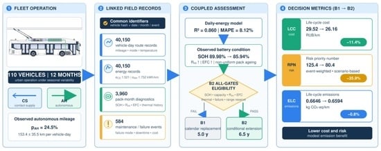
This study presents an empirical fleet-level assessment of 110 autonomous-range trolleybuses using anonymized records collected over 12 months. The dataset comprises 40,150 vehicle-day operating records, 40,150 energy records, 3960 pack-month SOH records, and 584 maintenance, failure, and downtime events. Outcomes are reported in absolute units: RUB/km for LCC, kg CO2-eq/km for ELC, events per 100,000 km, and downtime hours per 10,000 km. Autonomous operation accounted for 24.5% of mileage. Average net energy consumption was 1.520 kWh/km, whereas mode-distributed gross energy was 1.521 kWh/km in contact-supply mode and 1.752 kWh/km in autonomous mode. The daily-energy model achieved a full-sample fit of R2 = 0.860 and MAPE = 8.119%. Validation of vehicle-grouped data using the generated dataset showed R2 = 0.842 and MAPE = 8.74%. Mean SOH decreased from 89.98% to 85.94%, accompanied by higher internal resistance. In the central 6.5-year scenario, diagnostic-gated strategy B2 reduced estimated LCC from 29.52 to 26.16 RUB/km. The event-weighted control effect by RPN decreased from 125.4 to 80.4 (35.9%). Baseline ELC decreased only from 0.6646 to 0.6594 kg CO2-eq/km because operational electricity dominated the total. The contribution is an observation-linked framework that integrates vehicle-day operation, pack-month diagnostics, and event-level maintenance data to compare cost, emissions, and risk under explicit battery-eligibility and service-coverage constraints. The novelty is therefore the empirical, observation-level coupling and joint calibration of existing energy, battery-condition, life-cycle, and reliability methods within one auditable fleet workflow, rather than the introduction of a new standalone degradation or reliability model.

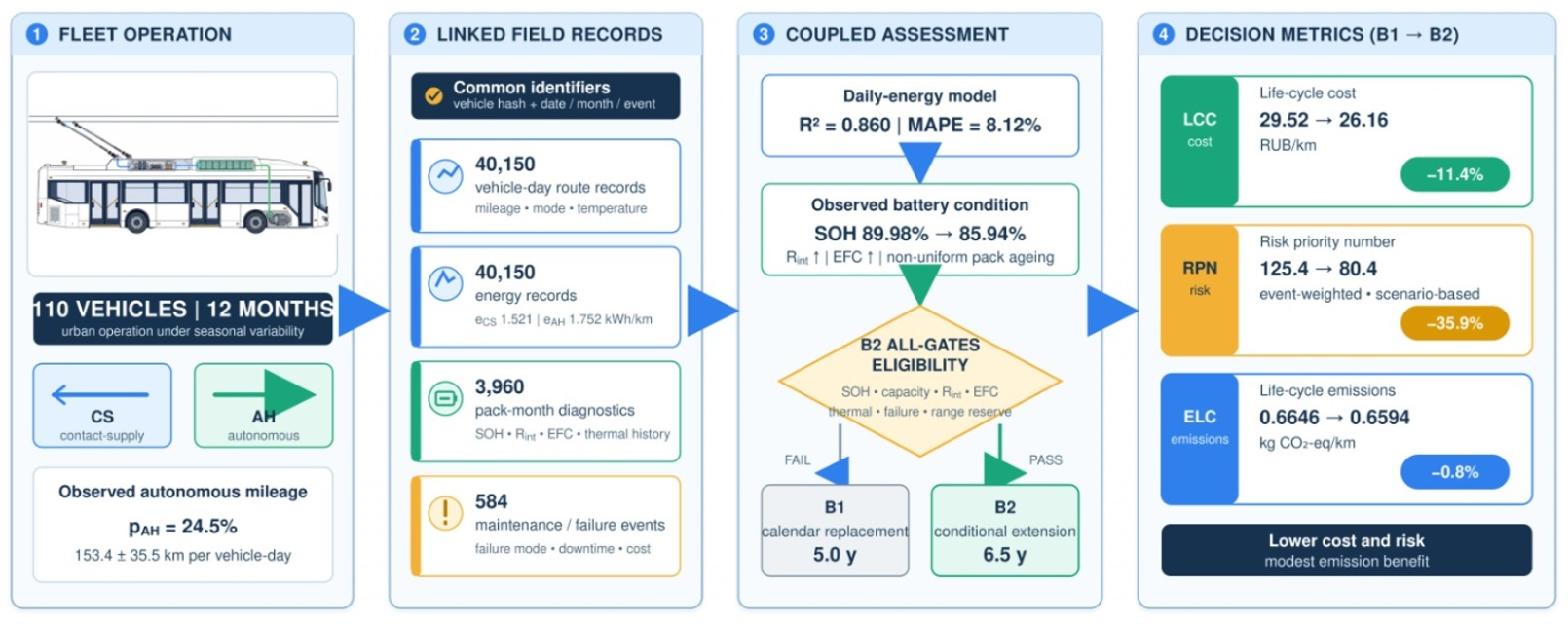
Graphical Abstract

1. Introduction

The decarbonization of urban mobility, increasing requirements for public-transport availability, and the modernization of transport infrastructure create engineering tasks in which rolling stock must be evaluated using life-cycle, resource, environmental, and risk indicators in addition to specific energy consumption [1,2]. Urban-mobility roadmaps and transport-planning reviews likewise emphasize infrastructure and implementation constraints in sustainable mobility transitions [3,4]. For municipal authorities and fleet operators, the critical outcomes are life-cycle cost, vehicle availability, battery service life, reliability of high-voltage components, unplanned-downtime risk, and the environmental consequences of operation and replacement of material-intensive components [5,6,7,8]. Reliability-oriented engineering models likewise stress system-level failure consequences and component interactions [9,10]. These outcomes depend not only on vehicle design but also on route structure, power-supply mode, climate, catenary condition, maintenance practice, and the completeness of operational telemetry [11].
An autonomous-range trolleybus occupies an intermediate position between a conventional trolleybus and a battery–electric bus. It remains connected to the catenary network where infrastructure is available, while onboard energy storage enables operation through network gaps and on route extensions without overhead supply [12,13,14]. Autonomous operation therefore constitutes a distinct transport and energy function that changes energy demand, battery cycling, maintenance requirements, and operational risk [15,16].
Autonomous operation cannot be regarded as a cost-free route extension. It introduces additional battery cycling and conversion losses across the catenary–charger–battery–power-electronics–traction chain, while increasing sensitivity to ambient temperature, HVAC demand, battery cooling, converter loading, and high-voltage insulation conditions. Auxiliary-system power demand is also a material contributor to electric public-transport energy use [17]. The permissible autonomous mileage share pAH must therefore reflect route demand, energy efficiency, remaining ESS life, pack-specific diagnostic status, failure risk, downtime cost, and the maturity of the operator’s data infrastructure [18]. Comparable energy-storage control studies likewise show that reliability gains depend on constrained, data-driven operating policies [19]. An autonomous-range trolleybus should consequently be evaluated as an integrated route–energy–battery–maintenance–risk system rather than as a conventional trolleybus fitted with an auxiliary battery [20,21].
Previous research on electric buses, trolleybuses, and battery–electric vehicles has developed several mature but largely separate analytical streams, including operational energy modelling, life-cycle cost assessment, environmental assessment, battery SOH and degradation analysis, and reliability- or FMEA-based evaluation [22,23,24,25,26]. These studies provide a methodological basis for each individual assessment layer, but they commonly use different observational units, datasets, and scenario assumptions. Consequently, autonomous-operation intensity may be quantified in the energy model without consistently propagating its consequences to battery conditions, maintenance burden, life-cycle cost, emissions, and failure risk.
The specific scientific gap addressed in this study is the absence, within the reviewed literature, of a fleet-level workflow that links vehicle-day operation, mode-resolved CS/AH energy telemetry, pack-month battery diagnostics, and event-level maintenance and failure records before calculating life-cycle and risk indicators. Without such linkage, it is difficult to distinguish whether higher energy consumption and battery degradation are associated with AH operation itself or with correlated factors such as seasonal conditions, route structure, passenger load, HVAC demand, EFC accumulation, and thermal history [27,28,29]. When these variables are evaluated in separate models or only through annual averages, the burden attributed to autonomous operation may be confounded with climatic, operational, and degradation-related effects [30].
This study addresses the identified gap through a common linked data structure and a sequential data-to-decision workflow. Daily mileage and energy records are first reconciled at the vehicle-day level; SOH, internal resistance, EFC, available capacity, and temperature events are evaluated at the pack-month level; and maintenance, failure, downtime, and cost consequences are retained at the event level. These layers are subsequently propagated into absolute fleet-level decision metrics—RUB/km, kg CO2-eq/km, events/100,000 km, downtime h/10,000 km, and weighted RPN—rather than being compared only through independently parameterized or normalized scenario indicators [31,32,33,34,35].
A linked 12-month database was first formed for 110 autonomous-range trolleybuses, comprising 40,150 vehicle-day operating records, 40,150 energy records, 3960 pack-month SOH records, and 584 maintenance, failure, and downtime events. After data-quality control, the distributions of Ltotal, LCS, LAH, pAH, eavg, eCS, eAH, SOH, Rint, EFC, downtime, and failure modes were calculated. The daily-energy model was then checked against measured daily energy, and the resulting operational indicators were propagated to LCC, ELC, and FMEA calculations. This sequence replaces normalized indices with auditable absolute metrics: RUB/km, kg CO2-eq/km, events per 100,000 km, downtime hours per 10,000 km, and event-weighted RPN.
The central research question is how linked operational, energy, battery-diagnostic, and maintenance records can be used to determine whether a condition-based battery-life extension policy remains economically beneficial and risk-acceptable across the actual levels of autonomous operation, seasonal temperature, route heterogeneity, and battery conditions.
Accordingly, the aim of this study is to develop and empirically test a fleet-level assessment framework that links CS/AH operation, measured energy demand, battery SOH and internal resistance trajectories [36,37], maintenance and failure events, life-cycle cost, life-cycle emissions, and risk indicators. The object of this study is a fleet of 110 autonomous-range trolleybuses operated under pronounced seasonal and route variability. The analysis is based on 40,150 vehicle-day operating records, 40,150 energy records, 3960 pack-month diagnostic records, and 584 maintenance, failure, and downtime events.
The methodological contribution of the study is the observation-level coupling of five assessment layers that are commonly analyzed separately. First, net daily energy and mode-distributed CS/AH energy are retained as physically distinct quantities within a common energy balance. Second, the contribution of autonomous mileage is evaluated jointly with temperature, passenger load, route structure, and auxiliary demand rather than through a fixed autonomous-mode coefficient. Third, battery-life extension is formulated as a diagnostic-gated strategy based on SOH, internal resistance, cycling, thermal history, and failure events rather than as an unconditional calendar extension. Fourth, economic, environmental, and reliability outcomes are expressed in absolute fleet-level units and are derived from the same operational records [38].
The contribution is therefore integrative and empirical rather than based on a new standalone energy model, battery chemistry, SOH estimator, life-cycle assessment method, or FMEA procedure. Its novelty lies in the reproducible linkage and joint calibration of these analytical layers using the same fleet observations. This structure permits the economic benefit of the B2 strategy to be evaluated simultaneously with battery-condition constraints, energy consequences, and failure-risk requirements [39,40]. Accordingly, the claimed novelty is a systems-integration contribution: common identifiers, aligned observational units, and a shared decision layer enable cross-domain conclusions that cannot be obtained when the constituent methods are applied independently.
The remainder of the article is structured as follows. Section 2 describes the fleet, linked database, quality control procedure, CS/AH energy model, SOH–Rint–EFC diagnostic block, LCC and ELC calculations, FMEA, and the discrete multi-criteria scenario comparison. Section 3 reports operating distributions, seasonal energy patterns, energy-model validation, SOH and resistance trends, failure and downtime structure, LCC and ELC decomposition, FMEA results, scenario comparison, and sensitivity analysis. Section 4 discusses engineering interpretation, diagnostic eligibility for B2, environmental and economic limits, study limitations, and practical recommendations. Section 5 summarizes the principal findings.

2. Materials and Methods

2.1. Object of Research and Boundaries of the System

This study considers a fleet of autonomous-range trolleybuses of the “Gorozhanin” family operated in an urban network with pronounced seasonality [41]. The unit of observation is the vehicle-day for operational and energy data, the pack-month for battery diagnostics, and the maintenance, failure, or downtime event for reliability analysis [42]. The multi-level observation structure follows established empirical case-study design principles [43,44].
The functional unit is 1 vehicle-km of fleet operation. The system boundary includes vehicle operation, maintenance and repair, battery replacement or condition-based life extension, diagnostic procedures, residual value, and ESS recycling [45]. Traction-drive and vehicle-body manufacturing are excluded from the B1–B2 difference because these components are unchanged between the compared battery strategies [46]. The explicit system boundary also supports theory building from a bounded engineering case while retaining traceability of the compared alternatives [47,48].
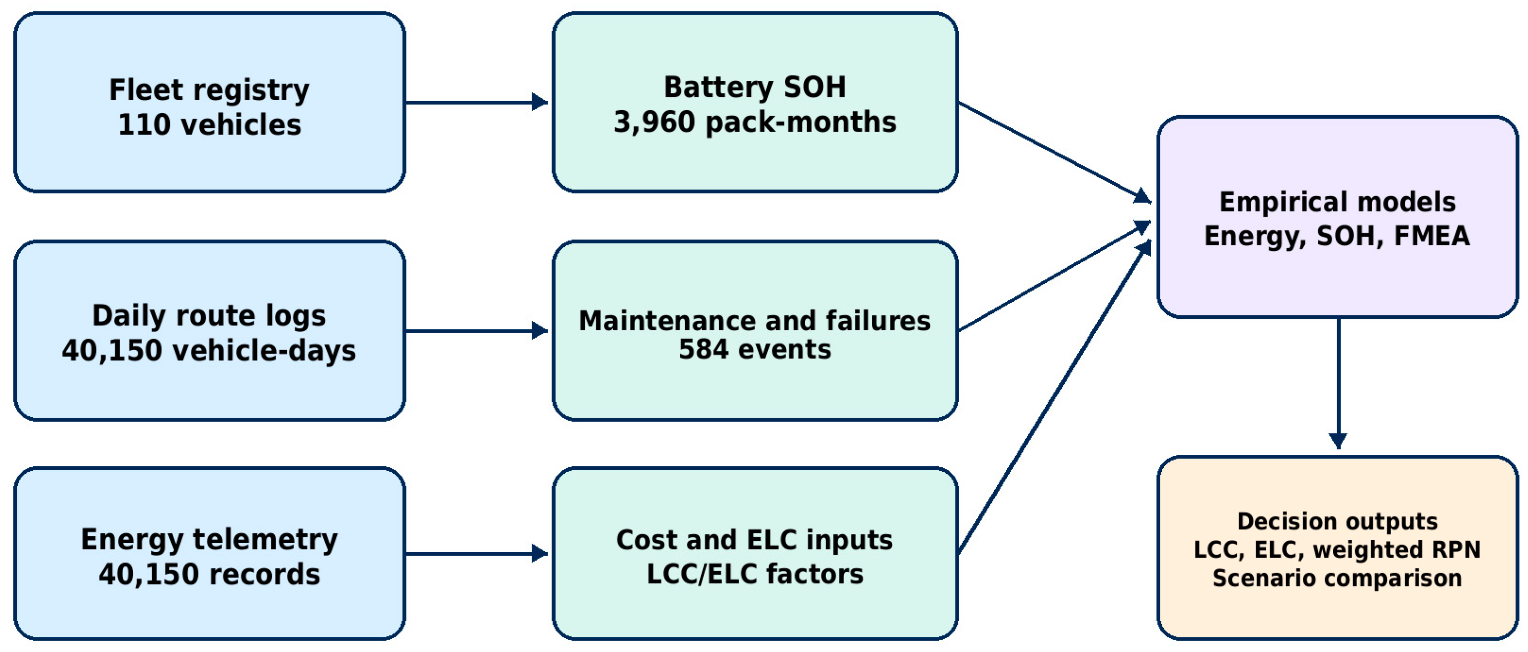
Figure 1 summarizes the data and calculation workflow. The procedure starts with verified operational records, proceeds through energy, battery, and failure models, and ends with LCC, ELC, event-weighted RPN, and a discrete multi-criteria scenario comparison. The workflow therefore separates measured records, statistically aggregated indicators [49,50], and B1/B2 management scenarios. This progressive case-study logic separates empirical evidence, analytical generalization, and decision-oriented interpretation [51,52,53].
Figure 1 shows that management scenarios are applied only after the operational, diagnostic, and event records have been linked and checked. This ordering improves traceability and reduces the risk of artificial precision when fleet-level conclusions are derived from disconnected assumptions [54].

2.2. Composition of the Empirical Database

Table 1 identifies the linked data blocks, their volumes, key fields, and roles in the fleet-level analytical workflow.
Table 1 shows that vehicle-day operating records are linked to energy telemetry, pack-month SOH diagnostics, event-level maintenance and failure data, and cost and environmental factors. This structure supports both B1/B2 scenario comparison and statistical analysis of seasonality, route heterogeneity, battery conditions, and failure burden.

Anonymization, Record Linkage, Preprocessing, and Uncertainty Reporting

Before the analytical tables were linked, direct identifiers were removed from the operator exports. Vehicle identifiers were replaced with irreversible vehicle hashes, and route identifiers were represented by generalized route codes. Personnel identifiers, internal asset numbers, commercially sensitive accounting fields, and information that could directly identify individual employees or operational counterparties were excluded. Vehicle-day records were linked by vehicle hash and operating date, battery-diagnostic records by vehicle hash, battery-pack code, and month, and maintenance or failure records by vehicle hash, event date, and event category. This study did not use personally identifiable information.
Preprocessing was performed separately for each analytical variable rather than by deleting an entire vehicle-day whenever one field was incomplete. Mandatory checks included date validity, non-negative mileage and energy values, non-zero denominators, consistency between total, CS, and AH mileage, and the availability of the corresponding vehicle identifier in the fleet registry. Target variables—daily energy, mileage, SOH, internal resistance, and event duration—were not imputed. If a noncritical auxiliary field was incomplete, the record was retained only for analyses that did not require that field. Records requiring verification were checked against the corresponding source log and neighbouring vehicle-day or vehicle-week records. Unresolved values were excluded only from the affected metric and retained in the data-quality log with the reason for exclusion.
Three forms of uncertainty were distinguished. First, empirical variability was reported using standard deviations, interquartile ranges, and 5–95% intervals. Second, predictive uncertainty of the energy model was characterized using MAPE, RMSE, residual diagnostics, and validation by operational subgroup. Third, data-quality uncertainty was represented by the record-status categories reported in Table 2. The original operator exports did not include complete calibration certificates for all onboard measurement channels; therefore, unsupported sensor-level uncertainty values were not assigned retrospectively. The reported uncertainty ranges characterize fleet variability and model error and should not be interpreted as manufacturer-certified instrument tolerances.
The record-status categories and the corresponding metric-specific preprocessing rules are summarized in Table 2. The categories refer to the 40,150 vehicle-day operational and energy records, whereas the separate data-quality log contains issue-level decisions and is not an additional set of vehicle-day observations.
Table 2 shows that 89.0% of the vehicle-day records passed the mandatory checks without correction. Partial records were not automatically discarded because many remained valid for analyses that did not require the incomplete auxiliary field. Conversely, a record was not retained merely because it belonged to the original export: values that could not be reconciled were excluded from the specific calculation affected by the inconsistency. This metric-specific rule preserved usable observations without imputing the principal energy, mileage, or battery-condition variables.
Representative anonymized fleet ranges are reported to make the empirical scale of the data transparent without disclosing commercially sensitive record-level information. Daily vehicle mileage was 153.4 ± 35.5 km per vehicle-day. The median autonomous-operation share was 26.3%, with an interquartile range of 18.8–31.1% and a 5–95% interval of 10.9–33.3%. Across the monthly aggregates, eavg ranged from 1.293 to 1.946 kWh/km, eCS from 1.388 to 1.771 kWh/km, and eAH from 1.608 to 2.056 kWh/km. Monthly mean SOH ranged from 85.94% to 89.98%, with monthly cross-pack standard deviations of 3.63–3.81 percentage points; mean internal resistance ranged from 14.92 to 15.83 mΩ, and mean EFC increased from 37.62 to 392.30. These values are calculated from anonymized operational observations and are not model-generated records.
The reported ranges describe between-record, between-vehicle, and seasonal variability. They are therefore distinct from instrument calibration uncertainty. Model-related uncertainty is reported separately through prediction errors and residual diagnostics, while record-level limitations are represented by the quality categories and metric-specific exclusions defined above.

2.3. Calculation of Operational and Energy Indicators

For the transition from primary operation logs to life-cycle indicators, each record was considered at the vehicle-day level, that is, as a daily operational implementation of a particular trolleybus [55]. For record j, the total mileage L total , j , mileage in the power-supply mode from the contact network L CS , j , mileage in autonomous mode L AH , j , daily electricity consumption E total , j , and mode-distributed energy components were recorded as E CS , j and E AH , j , recovered energy E regen , j , as well as the energy of auxiliary systems E HVAC / aux , j .
L total , j = L CS , j + L AH , j .
The actual autonomous-operation share for each daily record was determined as
p AH , j = L AH , j L total , j ,
where p AH , j is the observed share of autonomous mileage in daily transport work; L AH , j is mileage in autonomous mode, km; L total , j is the total daily mileage, km. Unlike the passport limit “up to 30 km of autonomous travel”, the value p AH , j was not set normatively but was extracted from the actual structure of the route, shift, and autonomous sections. Therefore, in further calculations p AH , j , it was considered as an empirically observable variable [56], reflecting the real operating mode [57], and not as a predetermined scenario parameter.
The average specific energy of daily operation was calculated as
e avg , j = E total , j L total , j ,
where e avg , j is the average specific energy, kWh/km; E total , j is measured daily net energy, kWh; L total , j is the total daily mileage, km. e avg was further used in the LCC and ELC calculations, as it corresponds to the energy actually taken into account by the operator when estimating operating costs and carbon footprint.
To characterize the power-supply modes separately, the specific energies in the CS and AH modes were additionally calculated:
e CS , j = E CS , j L CS , j ,
e AH , j = E AH , j L AH , j ,
where e CS , j is the specific energy of motion when powered from the contact network, kWh/km; e AH , j is the specific energy of autonomous motion, kWh/km; E CS , j and E AH , j are mode-distributed energy components, kWh; L CS , j and L AH , j are the corresponding mileages, km. A mode-specific energy indicator was not calculated when its corresponding mileage denominator was zero, negative, or unresolved after verification. Such a record was excluded only from the affected ratio—for example, from eAH when LAH = 0—and could remain available for other valid calculations. Each metric-specific exclusion was retained in the data-quality log together with the affected variable and the reason for exclusion.
It is fundamentally important that e avg , e CS , j , and e AH , j are not three interchangeable ways of describing the same energy. In this work, e avg refers to the measured daily net energy, while it characterizes e CS , j   e AH , j the mode-distributed gross energy of motion before the final accounting of recuperation and auxiliary loads. Therefore, the energy balance of the daily recording was given in the form of
E total , j = E CS , j + E AH , j E regen , j + E HVAC / aux , j + δ E , j ,
where E total , j is the measured daily net energy, kWh; E CS , j is the energy related to the movement in the contact-network mode, kWh; E AH , j is the energy related to autonomous motion, kWh; E regen , j is the recovered energy, kWh; E HVAC / aux , j is the energy of HVAC and auxiliary systems, kWh; δ E , j is the residual member of the energy balance, including rounding, measurement errors, and time boundary mismatches of individual telemetry channels. With correct data synchronization, δ E , j should remain small compared to E total , j .
Such a notation eliminates the apparent discrepancy between e avg , e CS , and e AH . The average value e avg does not have to be a simple linear mixture, e CS and e AH , since it normalizes the net energy, which already includes the effect of recuperation and auxiliary systems. At the same time, e CS   e AH , it is possible to assess the difference in driving modes, including the increased energy load of the autonomous sections associated with the storage cycle, route profile, temperature, and operation of auxiliary consumers [58].
To test the energy model, a regression formulation was used, in which the dependent variable was the daily energy in absolute units, kWh:
E day , j = β 0 + β 1 L total , j + β 2 L AH , j + β 3 L total , j D cold , j + β 4 L total , j D hot , j + + β 5 L total , j I medium , j + β 6 L total , j I high , j + ε j .
Here, E day , j is the calculated or measured daily energy, kWh; β 0 is a free term that reflects the inevitable daily energy expenditure that is not scalable directly with mileage; β 1 is the basic mileage component of energy consumption, kWh/km; β 2 is the additional energy contribution of autonomous mileage, kWh/km; L total , j is the total daily mileage, km; L AH , j is the autonomous daily mileage, km; D cold , j is the cold load indicator; D hot , j is the heat load indicator; I medium , j and I high , j are binary indicators of medium and high passenger/mass load, respectively; ε j the coefficient β 3 characterizes the additional energy associated with the cooling load and has the dimension kWh/(km·°C); it shows the increase in energy consumption by 1 km when the temperature decreases by 1 C below the accepted reference level. The coefficient β 4 similarly describes the additional energy at the heat load above the reference temperature level and also has the dimension kWh/(km·°C). β 5 and β 6 reflect the effect of the vehicle load: β 5 sets additional energy per 1 km at an average load, and β 6 at a high load relative to the basic category of low load. Therefore β 3 and β 4 are interpreted as temperature–mileage coefficients, and β 5 and β 6 as mileage corrections for the operating load.
Temperature variables were calculated using formulas
D cold , j = max ( 0 , 18 T j ) ,
D hot , j = max ( 0 , T j 20 ) ,
where T j is the average daily outdoor temperature, °C; D cold , j is the cold-degree component, °C; D hot , j is the hot-degree component, °C. The first value describes the additional energy load at low temperatures associated with cabin heating, battery temperature preparation, and increased losses in electrical components. The second value reflects the additional load at high temperatures associated with air conditioning, ventilation, and thermal limitation of the storage device [59].
Binary load indicators were set as follows:
I medium , j = 1 , if   the   entry   is   related   to   average   load , 0 , in   other   cases .
I high , j = 1 , if   the   entry   is   related   to   high   load , 0 , in   other   cases .
The low-load category was used as a base and therefore was not introduced as a separate indicator to avoid a linear relationship between dummy variables. The coefficients β 5 and β 6 show the additional energy per 1 km at medium and high load relative to the baseline.
The choice of the model for E day , j , rather than directly for e avg , is due to the fact that daily energy is the primary measurable quantity and correctly scales with mileage. After evaluating the model, the predicted specific energy can be obtained as
e ^ avg , j = E ^ day , j L total , j ,
where the first term is the predicted daily energy from the regression model, kWh, and the second is the corresponding predicted specific energy, kWh/km. This two-stage formulation preserves the physical interpretation of the daily energy balance while providing the kWh/km indicator required for subsequent LCC and ELC calculations.
The regression is intentionally parsimonious and linear in its parameters. It does not explicitly resolve traffic congestion, stop density, road gradient and surface conditions, intersection delay, acceleration and braking style, driver-specific behaviour, catenary-voltage variation, or nonlinear interactions among route, temperature, passenger load, and battery conditions. Route grouping and subgroup validation capture only part of this heterogeneity. Accordingly, the AH-mileage coefficient is interpreted as an adjusted fleet-level association within the observed operating domain, not as a universal causal or physics-complete coefficient. Future work should compare generalized additive, mixed-effects, and tree-based models using route geometry, traffic state, speed and acceleration traces, and driver-level random effects.

Energy-Model Validation, Statistical Inference, and Subgroup Analysis

To prevent information leakage caused by repeated vehicle-day observations, the revised validation design assigns all records from the same trolleybus to a single fold. A vehicle-grouped 10-fold scheme therefore keeps approximately 11 complete vehicle histories in each test fold and fits the model on the remaining vehicles. Coefficients, preprocessing rules, and categorical encodings are recalculated independently within each training fold.
Predictive accuracy is evaluated only from out-of-fold predictions using the coefficient of determination R2, mean absolute error MAE, root mean square error RMSE, mean absolute percentage error MAPE, and mean prediction bias:
M A E = 1 n | E j E ^ j | , R M S E = 1 n ( E j E ^ j ) 2 , M A P E = 100 n E j E ^ j E j , B i a s = 1 n ( E ^ j E j ) ,
where E j is measured daily net energy, kWh; E ^ j is the corresponding out-of-fold prediction, kWh; and n is the number of observations in the evaluated validation subset.
The out-of-fold errors are reported separately by season, daily autonomous-operation share, and route group. Seasons are defined as winter (December–February), spring (March–May), summer (June–August), and autumn (September–November). Daily AH-share classes follow the empirical quartiles: low (pAH ≤ 18.8%), medium (18.8% < pAH < 31.1%), and high (pAH ≥ 31.1%). Routes are divided into low-, medium-, and high-AH groups using tertiles of the annual route-level mean pAH.
Because records from the same trolleybus are not statistically independent, coefficient uncertainty is evaluated using vehicle-clustered robust standard errors. The reporting set comprises the coefficient estimate, clustered standard error, 95% confidence interval, two-sided p-value, and variance inflation factor. Residual diagnostics include residuals versus fitted values, standardized-residual quantiles, subgroup mean bias, and the dependence of absolute error on predicted daily energy. Ninety-five-percent prediction intervals are estimated by vehicle-cluster bootstrap resampling, and empirical coverage is compared with the nominal 95% level.

2.4. SOH Diagnostics, Cross-Check Procedure, and Degradation Indicators

For each pack-month observation, the diagnostic block retained battery age, the BMS-reported state of health, measured available capacity, internal resistance, equivalent full cycles, mean depth of discharge, maximum and minimum cell temperatures, thermal-event count, and the corresponding maintenance and failure history. Individual pack records were preserved throughout preprocessing and were not replaced by vehicle-level or fleet-level averages before the diagnostic checks were completed.
When a periodic capacity-check result was available, the capacity-referenced state of health was calculated as
S O H C j = 100 × C m e a s , j C n o m ,
where S O H C j is the capacity-referenced state of health for pack-month observation j, %; C m e a s , j is the measured available capacity obtained during the periodic capacity check, Ah or kWh; and C n o m is the corresponding nominal beginning-of-life capacity expressed in the same units.
The uncertainty of the capacity-referenced SOH was propagated as
u ( S O H C j ) = S O H C j × u ( C m e a s , j ) C m e a s , j 2 + u ( C n o m ) C n o m 2 ,
where u ( S O H C j ) is the standard uncertainty of the capacity-referenced SOH, percentage points; u ( C m e a s , j ) is the uncertainty of the measured available capacity; and u ( C n o m ) is the uncertainty associated with the nominal reference capacity.
The BMS-reported SOH was treated as an operational diagnostic estimate rather than as a self-validating ground-truth value. Where capacity-check data were available, the consistency between the two estimates was evaluated using
Δ S O H c a l , j = S O H B M S , j S O H C , j ,
where Δ S O H c a l , j is the BMS-to-capacity diagnostic discrepancy, percentage points; S O H B M S , j is the SOH reported by the onboard battery-management system; and S O H C , j is the capacity-referenced value.
Pack-to-pack dispersion was retained explicitly because the fleet-average SOH may conceal a limiting pack within one vehicle. For vehicle-level diagnostic screening, the limiting condition was characterized by the minimum pack SOH, maximum internal resistance, and maximum thermal-event count. The within-vehicle SOH spread was calculated as
Δ S O H p a c k , i , t = max k ( S O H i , k , t ) min k ( S O H i , k , t ) ,
where Δ S O H p a c k , i , t is the SOH spread between packs installed in vehicle i at time t, percentage points; S O H i , k , t is the SOH of pack k; and k denotes the individual battery packs associated with that vehicle.
Battery age was used as a proxy for calendar exposure, EFC and mean DoD as indicators of cyclic loading, and maximum/minimum cell temperatures and thermal-event counts as indicators of thermal history. The available fleet exports did not contain complete cell-level current trajectories, charging cut-off voltage histories, exact charge and discharge C-rates, or a manufacturer-resolved electrochemical identification for every pack. Consequently, these factors were not reconstructed retrospectively, and the observed SOH and resistance trajectories are interpreted as fleet-level diagnostic associations rather than as direct identification of one electrochemical degradation mechanism.
Electrochemical impedance spectroscopy was not part of the routine fleet dataset used in the present analysis. It is considered a potential future diagnostic extension because impedance-domain features can supplement capacity-based SOH checks and can support compact onboard SOH-estimation models [60,61]. The current B2 evaluation therefore remains based on the available multiparameter combination of SOH, measured capacity, internal resistance, EFC, DoD, temperature history, thermal events, and failure records.
The B2 decision was formulated as an all-gates eligibility rule rather than as a weighted average of favourable and unfavourable indicators. For each diagnostic criterion m, the binary eligibility indicator was defined as
I m , i , t = 1 if   criterion   m   is   satisfied , 0 otherwise . .
The overall B2 eligibility indicator was calculated as
G B 2 , i , t = m = 1 M I m , i , t ,
where G B 2 , i , t is the B2 eligibility indicator for vehicle i at diagnostic time t; I m , i , t is the pass/fail result for diagnostic criterion m; and M is the number of mandatory diagnostic gates. Battery-life extension was allowed only when G B 2 , i , t = 1. Failure of any mandatory gate resulted in suspension of B2 eligibility and transfer of the battery pack to additional diagnostics, derated operation, repair, or replacement.
The diagnostic gates used for the illustrative B2 decision workflow are summarized in Table 3.
Table 3 converts the B2 strategy from a general condition-based concept into an auditable pass/fail procedure. The 80% SOH threshold is treated as a minimum capacity-retention gate rather than as the only replacement criterion. A pack with SOH > 80% may still be rejected when internal resistance, degradation rate, pack imbalance, thermal history, autonomous-range reserve, or failure history is unacceptable. Conversely, the fleet-average SOH cannot be used to approve all vehicles because the B2 decision is made for the limiting pack associated with each vehicle.
The 6.5-year horizon is therefore not interpreted as a guaranteed physical battery lifetime. It is the central economic scenario evaluated only for packs that continue to satisfy every mandatory gate at successive quarterly reviews. The actual extension may be shorter when a diagnostic gate is violated.
The deterministic all-gates rule was selected for three practical reasons. First, it is directly auditable during workshop and quarterly fleet reviews. Second, it prevents a favourable indicator from compensating for a safety-critical failed gate. Third, the available 12-month dataset is insufficient to calibrate reliable failure probabilities or vehicle-specific hazard functions for every eligibility threshold. The resulting rule is therefore intentionally conservative and transparent rather than statistically optimal.
This design also has explicit limitations relative to probabilistic or risk-based approaches. Binary thresholds discard distance-to-threshold information, treat uncertainty near a cut-off discontinuously, do not model dependence among SOH, internal resistance, EFC, thermal history, and failure records, and cannot quantify the probability of safe operation over a future extension horizon. A probabilistic extension would estimate the conditional probability of safe operation to horizon h, propagate measurement uncertainty, and authorize B2 only when expected cost and risk remain below operator-defined limits. Such calibration requires multi-year post-implementation data containing false alarms, missed detections, withdrawals, and time-to-failure outcomes; these data were not available for the present study.

2.5. LCC, ELC, FMEA, and Multi-Criteria Scenario Comparison

Life-cycle cost was calculated in RUB/km as the sum of energy cost, maintenance and repair cost, downtime cost, the annualized battery replacement component, and condition-monitoring expenditure [62]. Strategy B1 used a fixed 5.0-year calendar-replacement horizon. Strategy B2 used a variable condition-based horizon hB2, evaluated from 5.5 to 7.0 years, with 6.5 years adopted as the central scenario rather than as a guaranteed service life.
The annualized battery replacement contribution was calculated as
C b a t t ( h ) = K b a t t h L a n n
and total LCC as
L C C ( h ) = C energy + C MRO + C down + C batt ( h ) + C diag ( h ) ,
where C batt ( h ) is the battery replacement contribution at service-life horizon h, RUB/km; K b a t t is the replacement cost of the battery set, RUB; L a n n is the annual fleet mileage, km/year; C energy is the energy-cost component, RUB/km; C MRO is the maintenance and repair component, RUB/km; C down is the downtime-cost component, RUB/km; and C diag ( h ) is the diagnostic and condition-monitoring component associated with horizon h, RUB/km.
Under B2, the adopted horizon was reassessed quarterly. If any mandatory criterion in Table 3 was not satisfied, the assumed horizon was truncated at the corresponding withdrawal, repair, or replacement date. Consequently, the LCC benefit of B2 was conditional on continued diagnostic eligibility.
Life-cycle emissions were calculated in kg CO2-eq/km by separating operational electricity, maintenance-material, and battery-related contributions. The operational term retained the monthly structure of energy use and grid emission factors rather than applying one annual factor to all records.
The operational contribution was calculated as
E L C o p = m E m E F g r i d , m L t o t a l ,
where E L C o p is the operational electricity contribution, kg CO2-eq/km; E m is measured fleet electricity use in month m, kWh; EFgrid,m is the month-specific grid emission factor, kg CO2-eq/kWh; and Ltotal is total fleet mileage, km.
For strategy s, total life-cycle emissions were calculated as
E L C s = E L C o p + E L C M R O + E L C b a t t , g r o s s , s ( 1 r r e c ) ,
where E L C M R O is the maintenance-material contribution, kg CO2-eq/km; E L C b a t t , g r o s s , s is the gross battery-production contribution for strategy s before end-of-life credit, kg CO2-eq/km; and r r e c is the assumed recycling credit fraction. Sensitivity was evaluated by scaling all monthly grid factors by 0.80 and 1.20 while preserving their seasonal pattern, by considering weighted grid factors from 0.200 to 0.600 kg CO2-eq/kWh, and by varying the recycling credit from 0% to 20%.
Only failure and defect modes F1–F5 were included in FMEA: F1, battery degradation; F2, battery thermal derating; F3, traction power-electronics failure; F4, high-voltage insulation or charging-contact fault; and F5, auxiliary or high-voltage control-system fault. Scheduled-maintenance events were retained in LCC, downtime, and availability calculations but excluded from RPN so that preventive activities were not treated as failures.
For failure mode k and strategy s, the risk priority number was calculated as
R P N k , s = S k O k , s D k , s ,
where S k is the severity score; O k , s is the occurrence score under strategy s; and D k , s is the detection score. Each score ranges from 1 to 10, and a lower detection score denotes a higher probability of identifying the developing fault before functional loss. Severity was held constant between B1 and B2 because diagnostic controls do not change the physical consequence of a failure once it occurs. B2 was allowed to change only occurrence and detection scores when a specific preventive or monitoring control was assigned to the failure mode.
The failure-event-weighted fleet indicator was calculated as
R P N w , s = k N k R P N k , s k N k ,
where N k is the observed number of events assigned to failure mode k.
The relative change was calculated as
Δ R P N w = 100 R P N w , B 1 R P N w , B 2 R P N w , B 1 .
The multi-criteria comparison used LCC, ELC, and failure-only event-weighted RPN as three criteria to be minimized. Six predefined combinations of AH intensity and battery strategy were evaluated. Scenario a was classified as dominating scenario b when its LCC, ELC, and weighted RPN were no greater than those of b and at least one criterion was strictly lower. This dominance check was applied only to the evaluated scenario set; it does not constitute continuous multi-objective optimization and does not generate an optimized frontier. Because AH intensity also determines transport coverage, numerical dominance was interpreted only after applying the required service-coverage constraint.


3. Results

3.1. Generalized Operational Profile of the Fleet

Table 4 reports the principal absolute operating and energy indicators used to characterize the fleet-level case study.
Table 4 shows that autonomous operation accounts for approximately one quarter of fleet mileage and that eAH exceeds eCS by 15.2%. AH operation is therefore not an energy-neutral addition to contact-network operation; it must be evaluated together with battery conversion losses, seasonal auxiliary demand, and the distribution of autonomous sections.
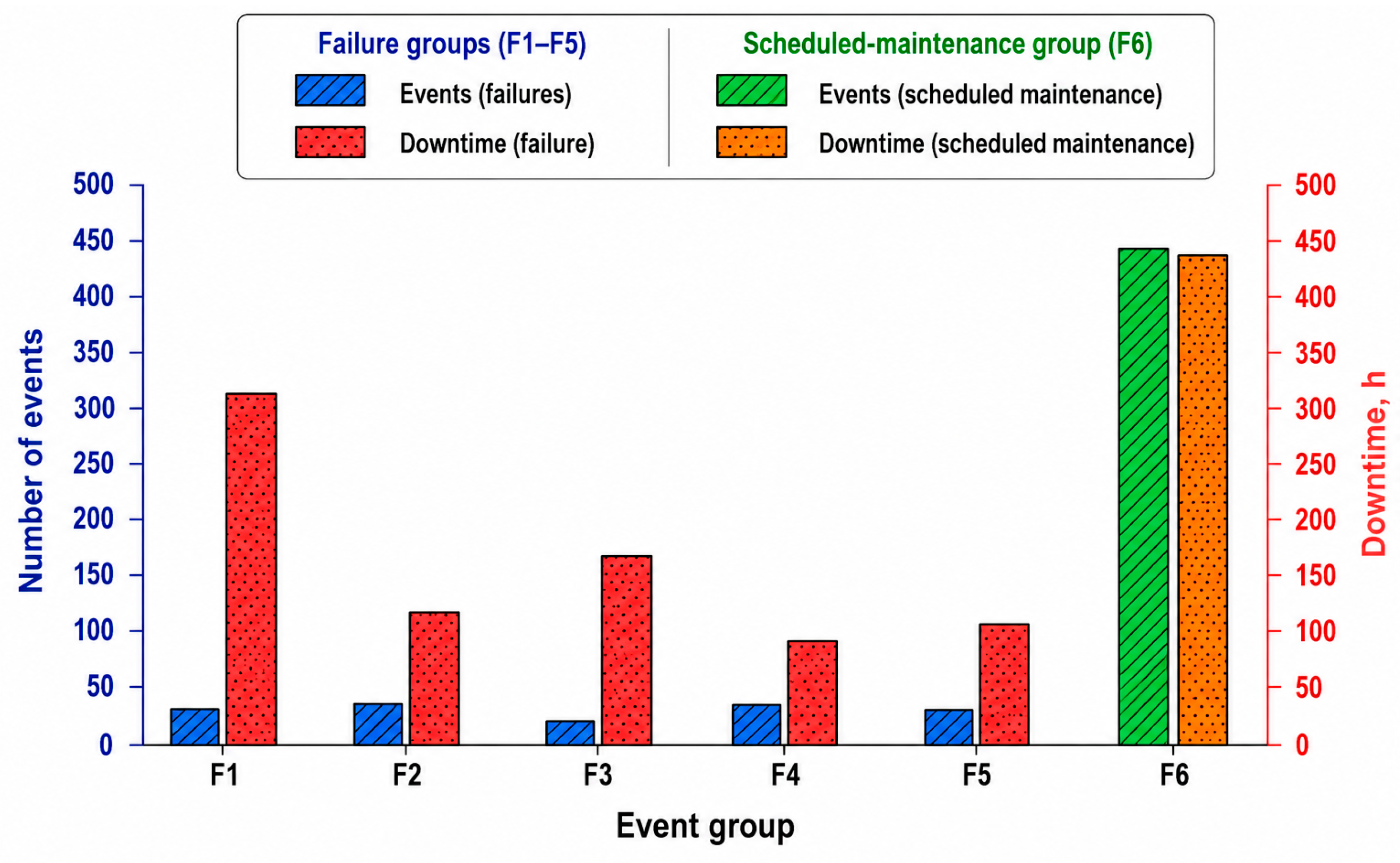
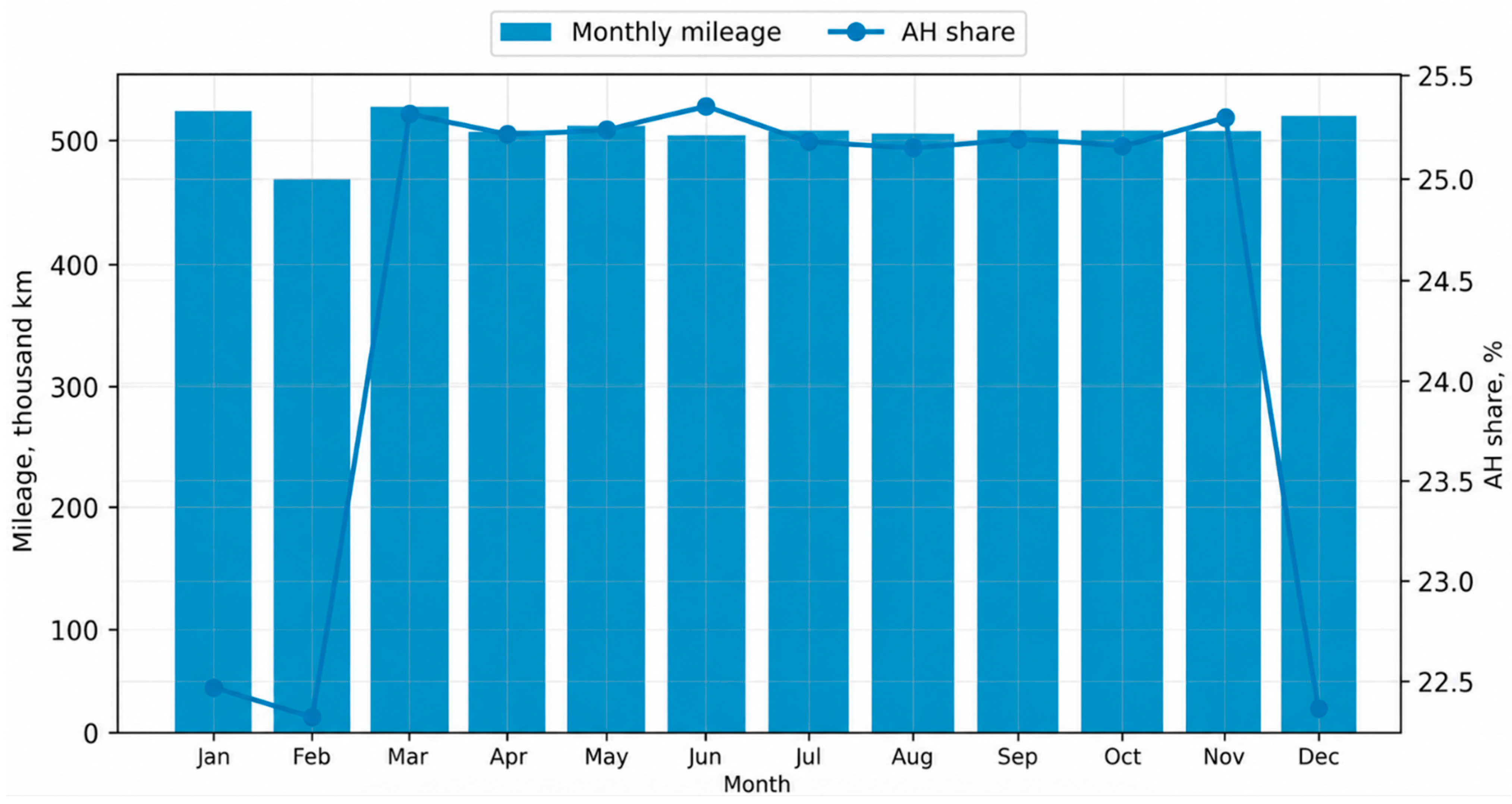
Figure 2 presents monthly fleet mileage and the observed autonomous-operation share. The persistence of pAH throughout the year confirms that AH operation is a regular transport function that must be included in LCC, ELC, and FMEA calculations.
Figure 2 shows that monthly mileage remains approximately 0.47–0.53 million km, while pAH varies from about 22% to 25%. The lower pAH in the coldest months is consistent with restricted autonomous operation and greater heating and auxiliary energy demand.
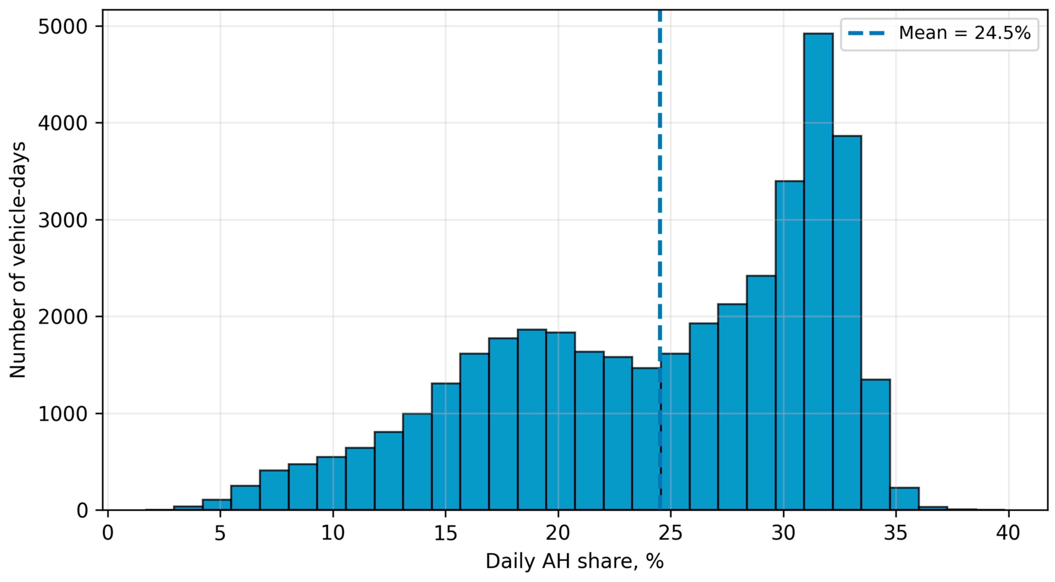
The distribution of pAH across all vehicle-day records was also examined because the annual mean can conceal route- and shift-level heterogeneity, as shown in Figure 3.
Figure 3 confirms that autonomous operation is distributed across a substantial proportion of vehicle-day records rather than being sporadic. Median pAH is 26.3%, the interquartile range is 18.8–31.1%, and the 5–95% interval is 10.9–33.3%. These results justify analysis of route- and shift-level variability in addition to the fleet mean.

3.2. Seasonality of Energy and Temperature Sensitivity

To reveal seasonality and the relationship between temperature and specific energy, Table 5 shows the monthly aggregates for mileage, pAH, temperature, eavg, eCS, eAH, HVAC, and recuperation.
Table 5 shows that the maximum eavg is in January and the minimum is in September. In winter, the increase in specific energy is accompanied by an increase in the share of HVAC/aux, while in the warm period, the relative share of recuperation increases. This confirms that the energy model must contain a temperature block, not just a pAH.
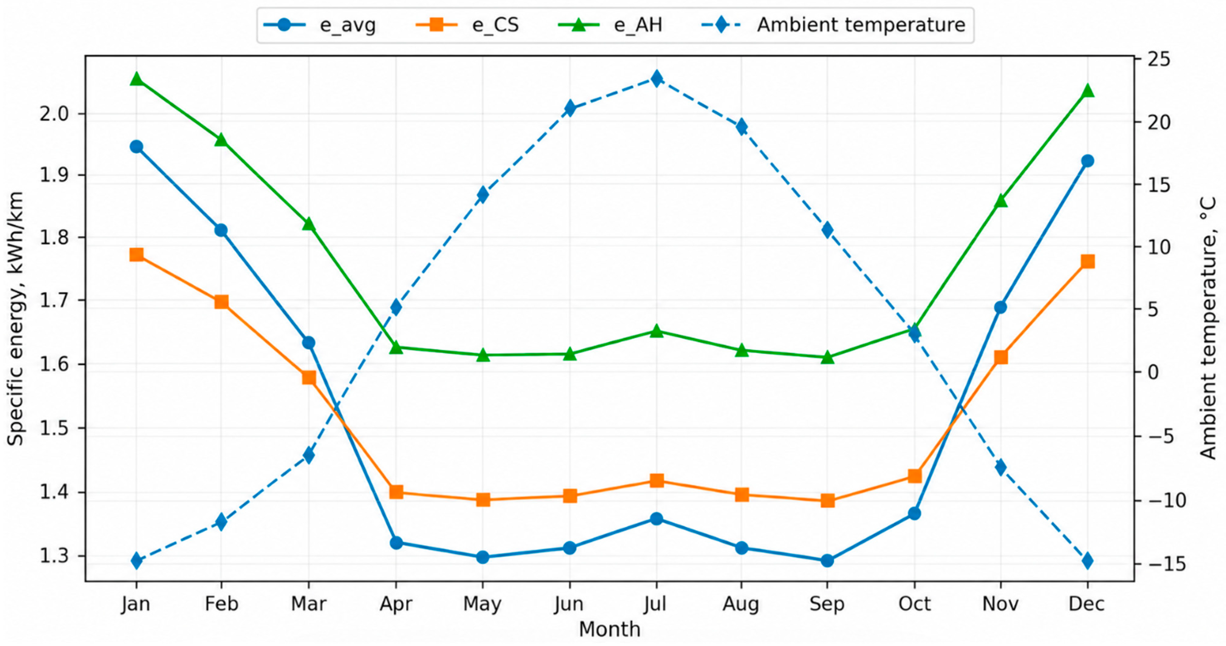
Figure 4 compares monthly eavg, eCS, eAH, and ambient temperature.
Figure 4 shows that eAH is consistently higher than eCS in all months. At the same time, the shape of the eCS and eAH curves is similar, which indicates a common seasonal factor—climatic load.
The difference between eAH and eCS reflects both battery conversion losses and the operating characteristics of autonomous sections, including stops, acceleration frequency, regenerative braking opportunity, and power limitations.
To quantify the contribution of mileage, AH mileage, temperature load, and passenger load, the daily-energy regression coefficients were estimated together with vehicle-clustered statistical inference. Table 6 reports the coefficient estimates, clustered standard errors, 95% confidence intervals, significance levels, and variance inflation factors.
Table 6 separates coefficient magnitude from statistical uncertainty. A predictor was interpreted as statistically distinguishable from zero only when its vehicle-clustered 95% confidence interval did not include zero. The variance inflation factors were used to verify that the separate effects of total mileage, AH mileage, temperature load, and passenger load were not dominated by excessive multicollinearity. The positive AH-mileage coefficient indicates an additional daily-energy contribution associated with autonomous operation after adjustment for total mileage, seasonal temperature load, and passenger load; however, this coefficient is interpreted as an adjusted association rather than an isolated causal effect. Overall out-of-fold performance and the stability of prediction errors across operational subgroups are reported in Table 7.
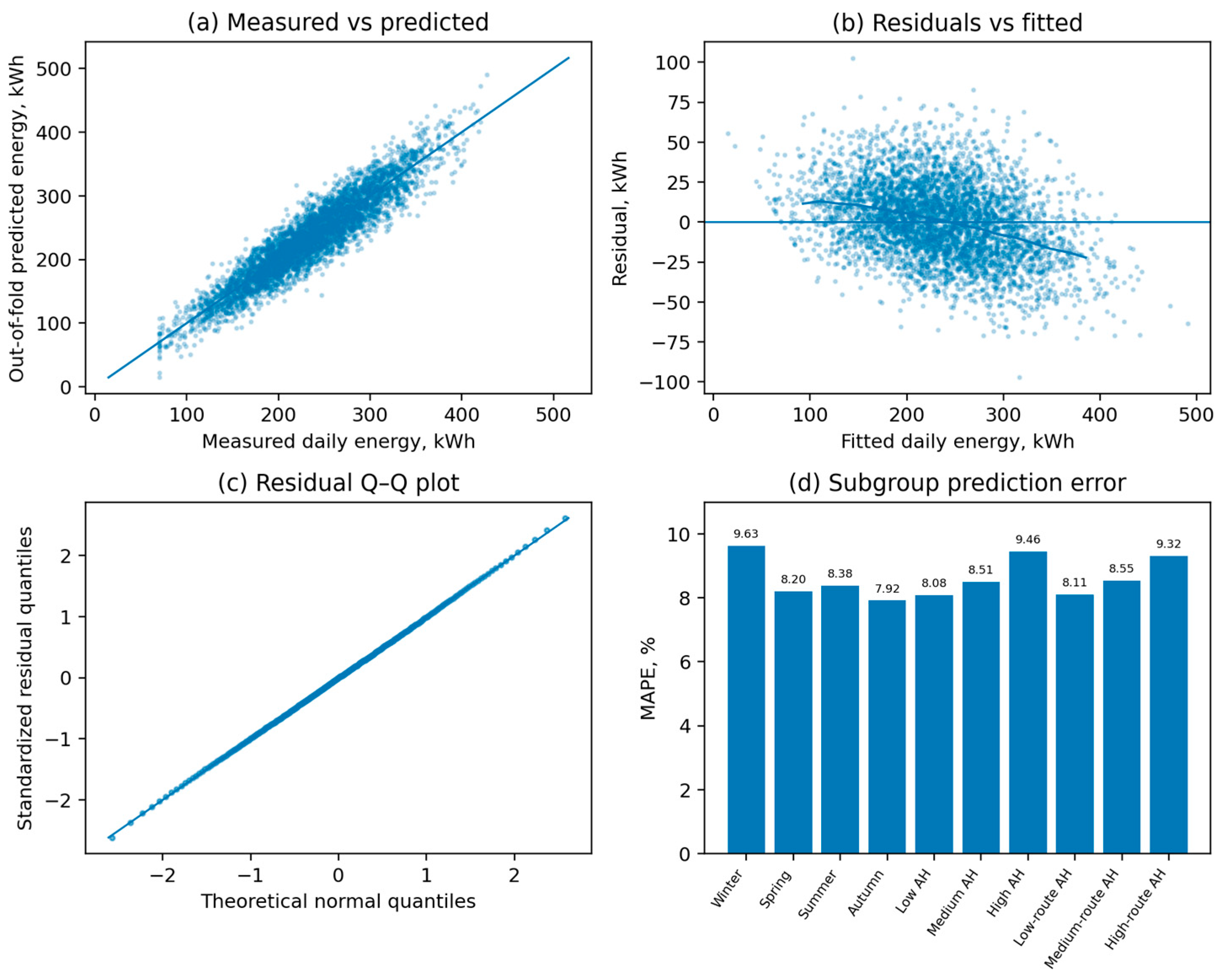
Table 7 shows that the overall illustrative grouped-validation result was R2 = 0.842, MAE = 19.64 kWh/day, RMSE = 25.18 kWh/day, and MAPE = 8.74%. Seasonal MAPE ranged from 7.92% in autumn to 9.63% in winter, while the range across daily AH-share classes was 8.08–9.46% and the range across route-AH tertiles was 8.11–9.32%. The largest error was observed in winter, whereas the smallest error occurred in autumn. This pattern is consistent with the higher variability of HVAC demand, battery thermal conditioning, and traction load under cold-weather operation. The illustrative prediction-interval coverage of 94.1% was close to the nominal 95% level, although coverage decreased to 92.9% for the high-AH subgroup.
Figure 5 summarizes the out-of-fold predictive performance and residual diagnostics of the vehicle-grouped validation procedure.
Figure 5a shows that the out-of-fold predictions remain concentrated around the 1:1 line, with the largest absolute deviations occurring in the upper daily-energy range. Figure 5b indicates mild heteroscedasticity without pronounced mean residual drift, while the mean out-of-fold bias was 0.18 kWh/day. Figure 5c shows limited tail departures from normality, indicating that extreme residuals are slightly heavier than the ones predicted by a Gaussian distribution. Figure 5d confirms that prediction accuracy was not uniform across all operating conditions: MAPE was highest in winter and lowest in autumn. Accordingly, the model is suitable for demonstrating the fleet-level LCC and ELC validation workflow within the illustrated operating domain, but subgroup-specific error must be retained when it is transferred to extreme seasonal or high-AH operating conditions.

3.3. Three-Dimensional Energy Surface pAH–T–eavg

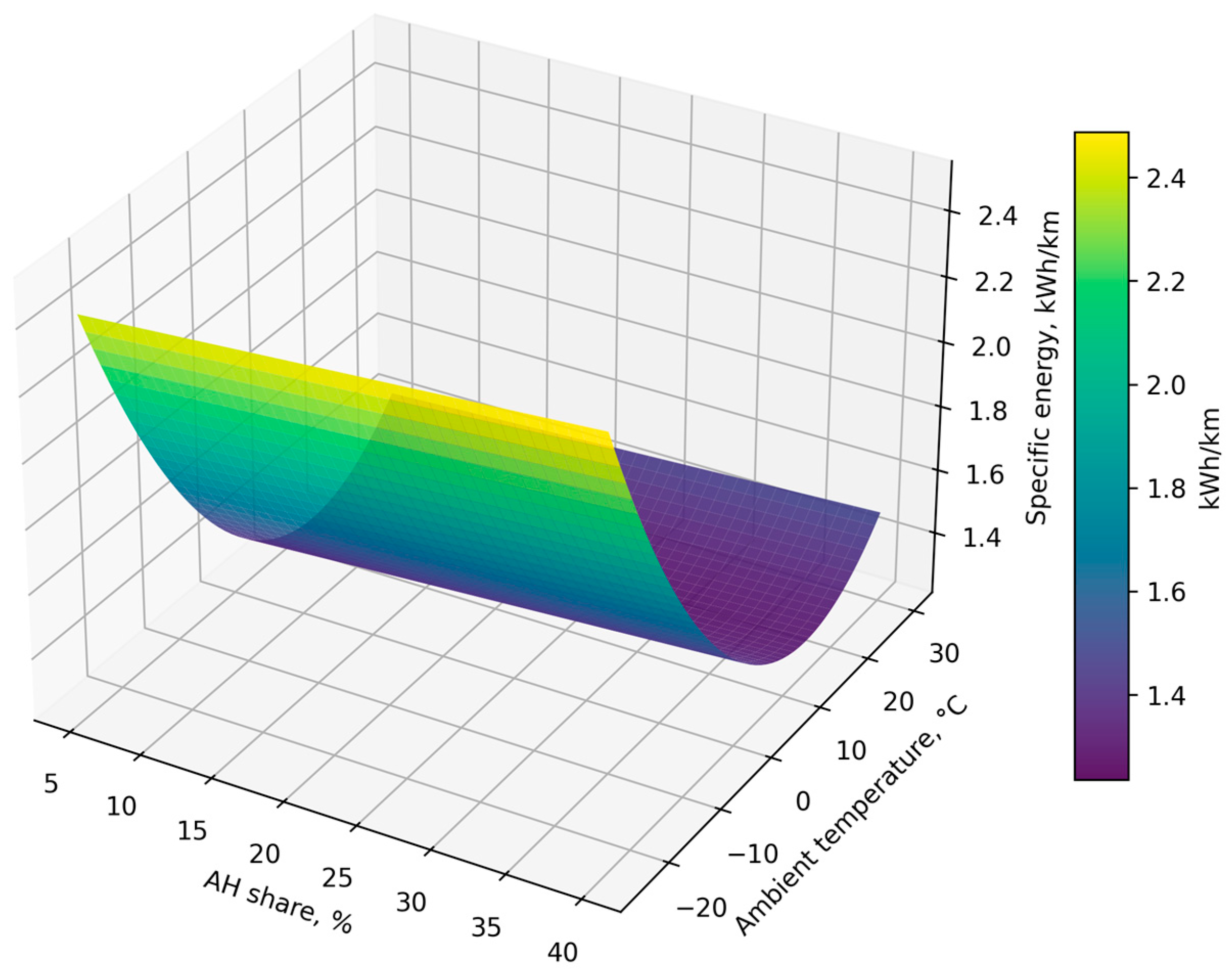
A three-dimensional fitted response surface was used to examine the joint association of eavg with pAH and ambient temperature. This visualization is useful because the energy effect of autonomous operation varies with climatic load.
Figure 6 shows that the lowest eavg values occur at moderate positive temperatures and low-to-medium AH shares. Under sub-zero conditions, eavg increases, and higher pAH is associated with an additional increase in specific energy consumption. Autonomous-operation intensity should therefore be evaluated jointly with seasonal temperature rather than as an independent route parameter.
Figure 6 also supports season-specific operating limits: the same pAH in January and September has different energy consequences. Route-planning rules should therefore include seasonal operating ranges rather than a single annual threshold.

3.4. Route and Inter-Vehicle Heterogeneity

To identify the routes that form the main load of the autonomous mode, Table 8 shows eight routes with the highest average pAH and their energy indicators.
Table 8 shows that routes with high pAH also have higher mean specific energy. The result demonstrates the need for route-level analysis because one fleet can exhibit materially different energy profiles depending on route assignment and the configuration of autonomous sections.
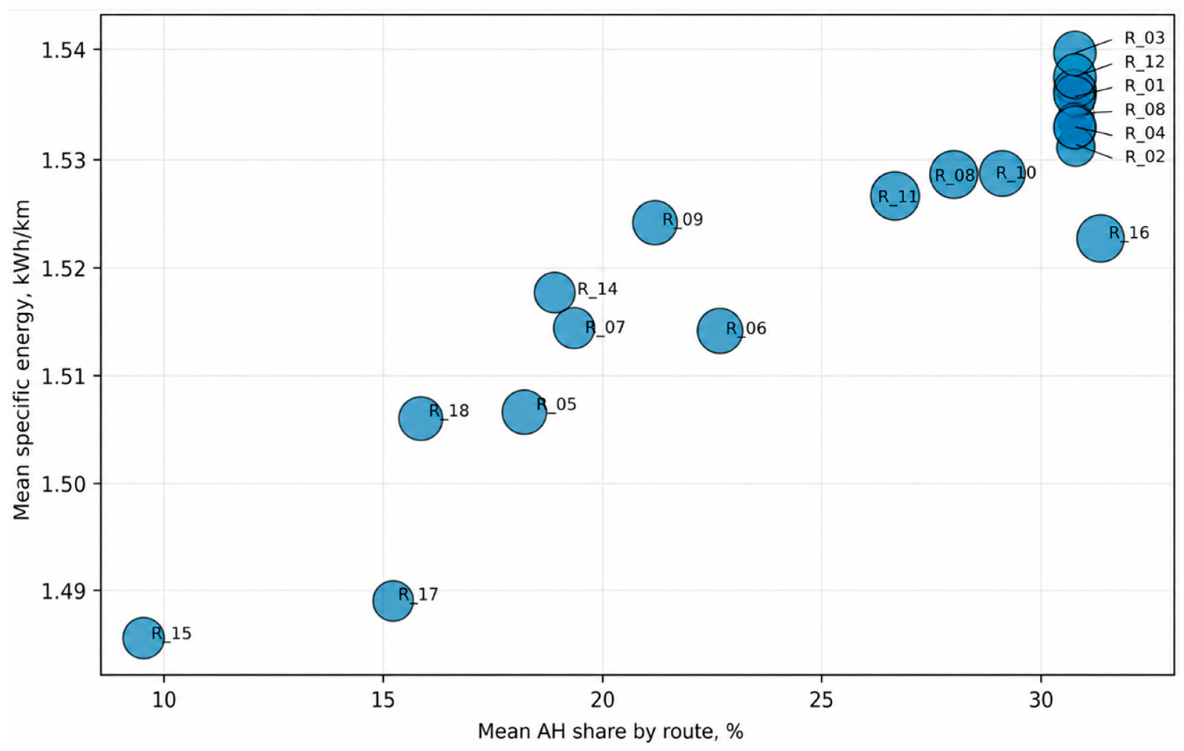
The relationship between route-level pAH and eavg is shown in Figure 7. The size of the point is proportional to the annual mileage of the route.
Figure 7 shows a strong positive route-level association between pAH and eavg. This does not imply that AH operation should always be minimized, because it extends service beyond the catenary network. Instead, the figure quantifies the energy cost of this transport function and supports service-coverage-constrained planning.
Table 9 summarizes inter-vehicle variability to determine whether fleet averages conceal materially different operating and SOH trajectories.
Table 9 shows substantial inter-vehicle differences in annual mileage and pAH, whereas annual mean specific energy varies less. The dominant differences are therefore associated with route assignment and operating intensity in addition to vehicle-specific conditions.
The minimum final SOH reported in Table 9 is 78.90%, which is below the illustrative 80% B2 eligibility threshold. Therefore, the observed fleet cannot be transferred to B2 as one homogeneous group. At least the limiting vehicle or battery pack requires additional verification and cannot be approved solely from the fleet-average SOH of 85.95%. This result illustrates why the proposed strategy is pack-specific and why economic savings calculated for the central B2 scenario should not be interpreted as automatic savings for every vehicle.
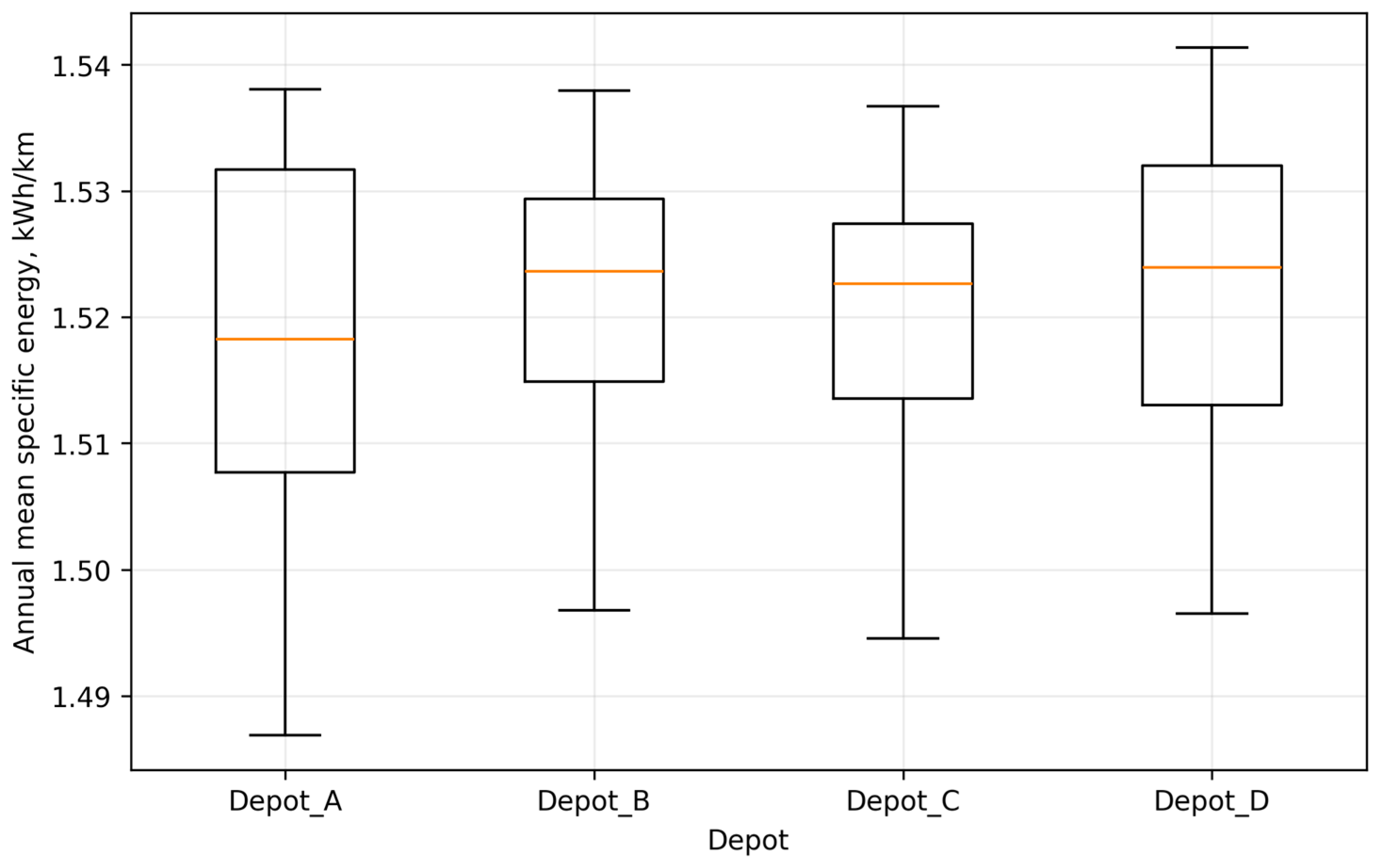
Figure 8 shows the distribution of annual mean specific energy by depot. The plot does not establish causality, but it identifies the organizational level at which route allocation, shift patterns, auxiliary-system control, storage conditions, and maintenance practice may contribute to differences.
Figure 8 shows that inter-depot differences are smaller than seasonal variability, although several vehicles remain outliers. These vehicles are candidates for targeted diagnostics because elevated eavg at comparable pAH may indicate deterioration of auxiliary systems, tyres, brakes, or contact-network interfaces.

3.5. Dynamics of SOH, Internal Resistance, and ESS Cycling

Table 10 reports monthly SOH, internal resistance, EFC, maximum cell temperature, and thermal-derating events for assessment of ESS service-life trends.
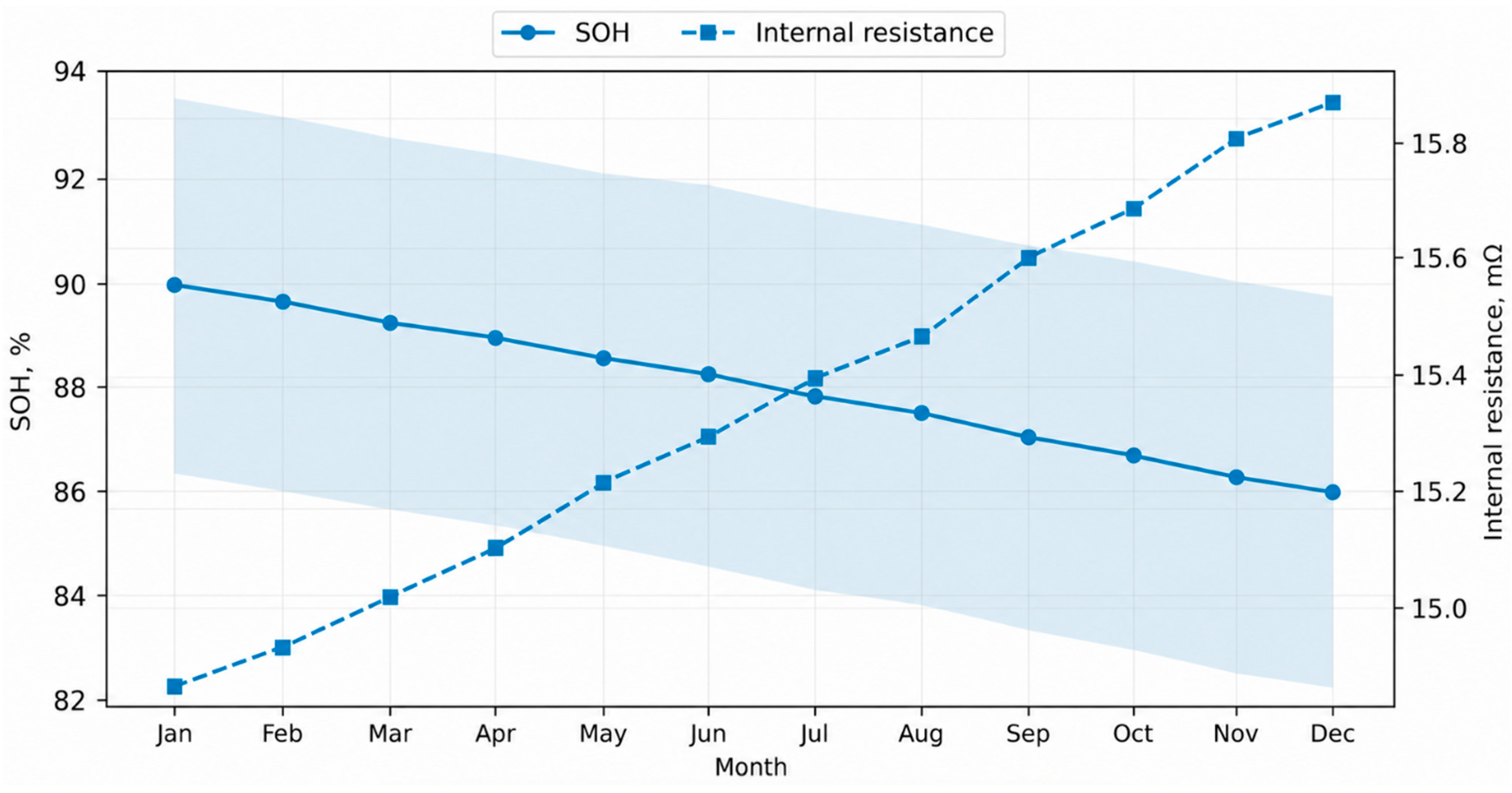
Table 10 shows a monotonic decrease in fleet-average SOH and an increase in EFC over the 12-month period. Mean SOH decreased from 89.98% to 85.94%, corresponding to 4.04 percentage points. The battery pack is therefore the principal service-life-limiting component of the autonomous-range trolleybus.
Table 10 reports both the monthly fleet mean and the between-pack standard deviation. The SOH standard deviation remains within 3.63–3.81 percentage points over the observation period, indicating that the annual mean decline of 4.04 percentage points should not be interpreted as a uniform degradation rate for every pack. Some packs therefore approach the limiting condition earlier than would be inferred from the fleet-average trajectory alone. This is the reason why the B2 screening procedure retains individual pack records and uses the limiting pack condition rather than only the monthly fleet mean.
The simultaneous decrease in SOH, increase in internal resistance, and accumulation of EFC are consistent with a mixed calendar–cyclic ageing pattern. However, the monthly aggregates do not uniquely distinguish loss of cyclable lithium, active-material degradation, electrolyte ageing, contact-resistance growth, or temperature-induced side reactions. The result is therefore used as a diagnostic trend for condition-based maintenance, not as direct electrochemical mechanism identification.
Figure 9 shows the average SOH and internal resistance by month. The shaded zone reflects the interblock spread of the SOH.
Figure 9 shows that declining SOH is accompanied by increasing internal resistance. SOH alone is therefore insufficient for service-life decisions because packs with similar SOH but different Rint may have different heat generation, voltage sag, and derating risk.
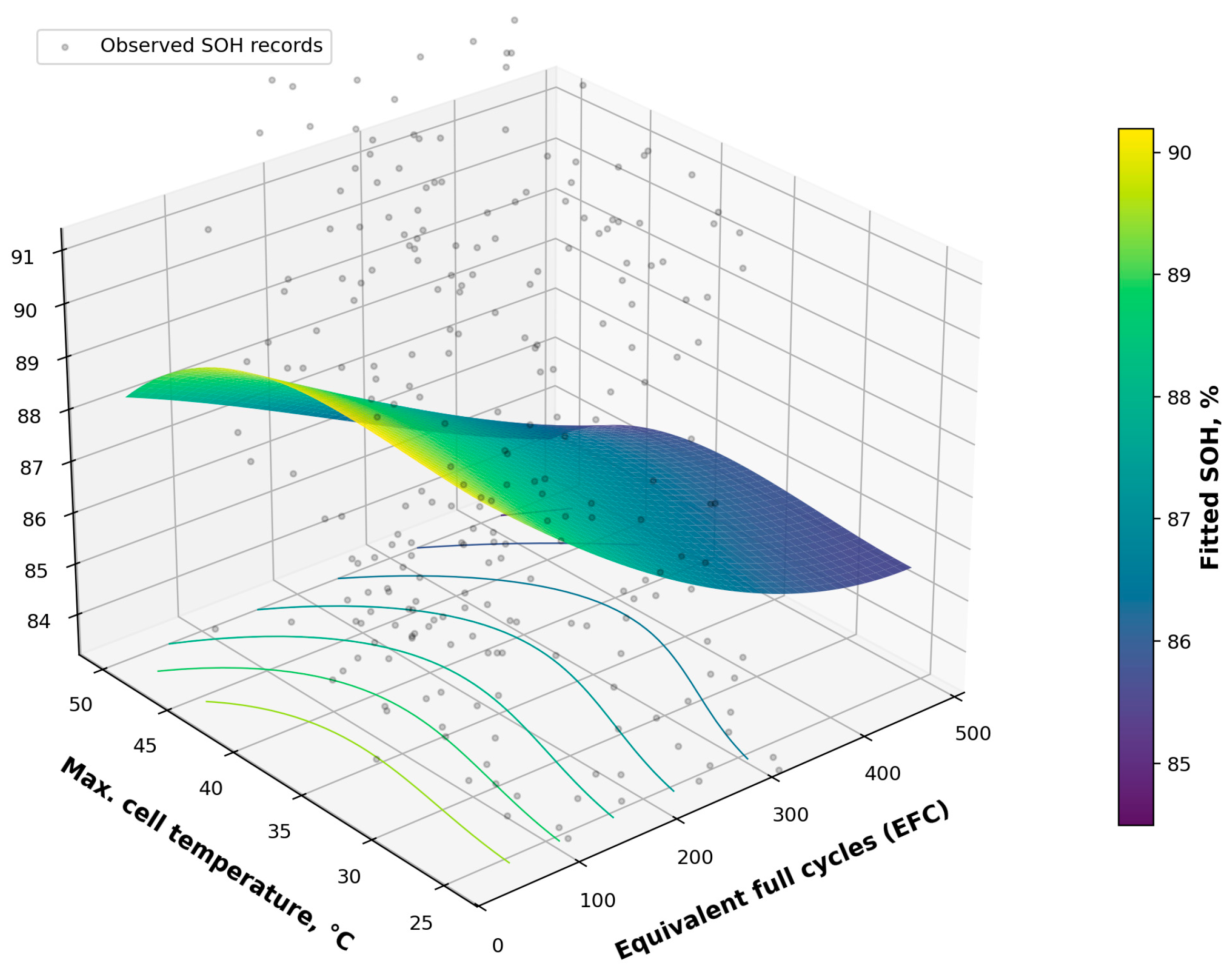
Figure 10 presents a three-dimensional nonlinear SOH response surface as a function of EFC and maximum cell temperature. Unlike a planar approximation, this representation illustrates the accelerating degradation trend associated with simultaneous increases in cyclic and thermal exposure.
Figure 10 shows a nonlinear fitted relationship among SOH, EFC, and maximum cell temperature. SOH declines gradually at low-to-moderate EFC, whereas the fitted surface becomes steeper at higher cyclic and thermal exposure. The surface supports joint consideration of EFC and temperature history in B2 screening but does not, by itself, identify a causal electrochemical mechanism.
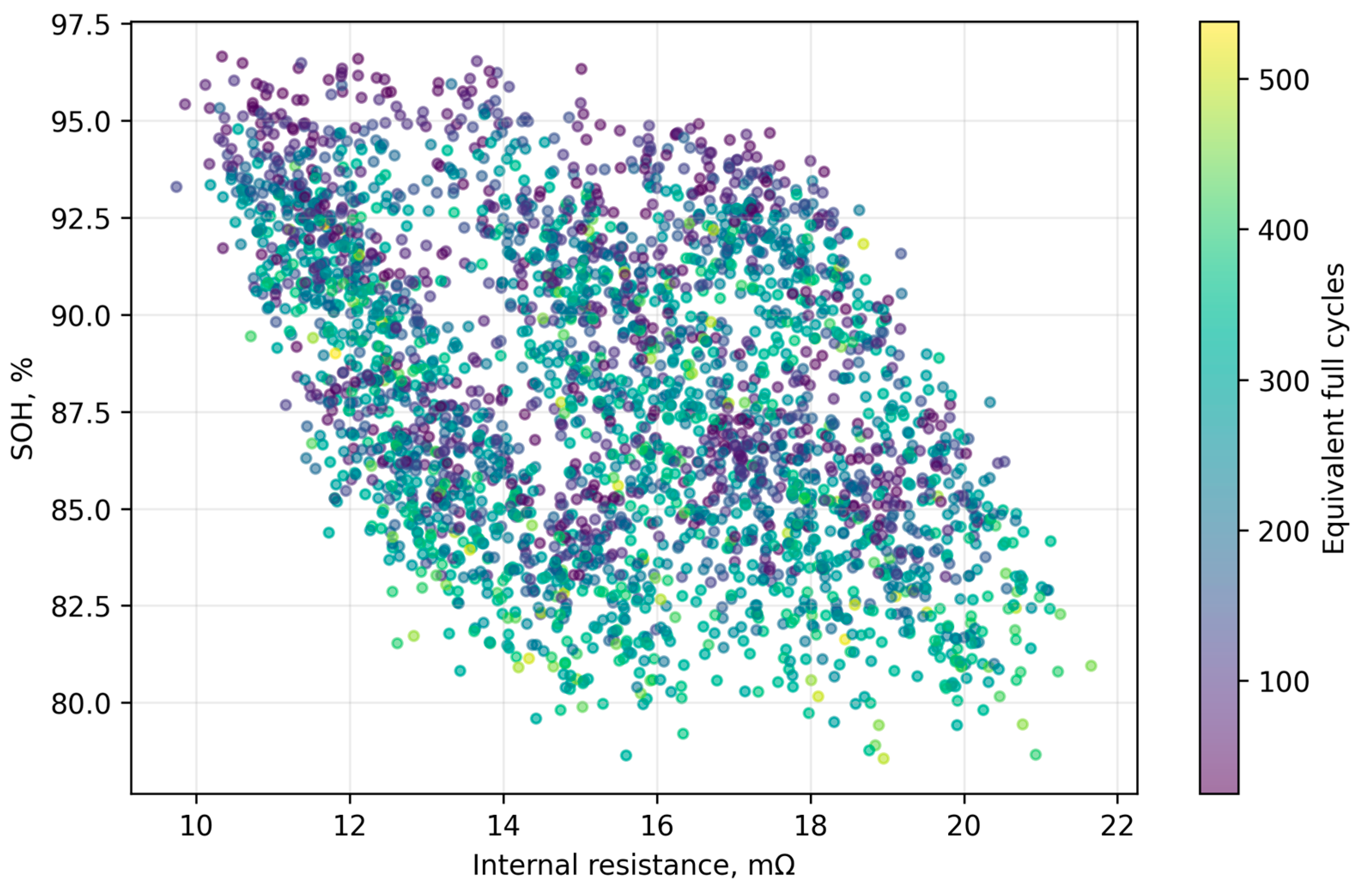
The relationship between SOH and internal resistance from individual pack-month observations is shown in Figure 11.
Figure 11 shows a negative association between SOH and Rint together with substantial dispersion. The B2 diagnostic gate must therefore combine SOH, internal resistance, thermal-event history, and measured-capacity verification rather than rely on one indicator.
The scatter in Figure 11 is also methodologically important. A given SOH value may correspond to different internal resistance levels and different accumulated EFC values, while a similar resistance value may occur for packs with different remaining capacities. Therefore, neither SOH nor internal resistance should be used as a single-variable replacement criterion. The figure supports a multiparameter diagnostic interpretation but does not establish that resistance growth alone caused the observed capacity loss.

3.6. Failures, Downtime, and Empirical FMEA

To make the FMEA reproducible, the score anchors were fixed before comparing B1 and B2. Table 11 defines the severity, occurrence, and detection scales used in the analysis.
Scores from 1 to 10 serve as engineering benchmarks for this decision-making model. The event rate metric uses the observed frequency of events along with recurrence or seasonal clustering.
Table 11 separates the three FMEA dimensions. Severity reflects the consequence after failure, occurrence reflects the observed frequency band and recurrence pattern, and detection reflects the probability of identifying the developing condition before service interruption. The same anchors were applied to both strategies.
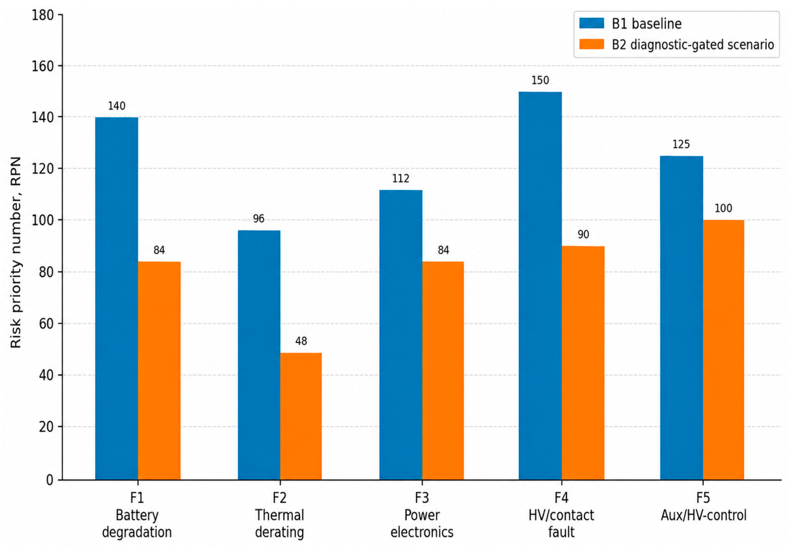
Table 12 makes the origin of every RPN explicit. Severity remains unchanged between strategies. For F1, B2 reduces occurrence from 5 to 4 and detection from 4 to 3 through capacity checks, SOH-trend monitoring, and resistance screening. For F2 and F4, thermal and high-voltage controls reduce occurrence, while F3 and F5 primarily benefit from improved detection. These changes are scenario assumptions rather than observed post-B2 frequencies.
The 144 observed failure events provide the weights for the fleet indicator. The B1 value is (28 × 140 + 33 × 96 + 20 × 112 + 34 × 150 + 29 × 125)/144 = 125.368. The B2 value is (28 × 84 + 33 × 48 + 20 × 84 + 34 × 90 + 29 × 100)/144 = 80.389. Therefore, the modelled reduction is 100 × (125.368 − 80.389)/125.368 = 35.87%, reported as 35.9%. Scheduled-maintenance events are excluded from both the numerator and denominator.
Figure 12 compares failure and scheduled-maintenance event counts with total downtime by event group. It separates frequent scheduled interventions from less frequent but operationally consequential failures.
Figure 12 shows that scheduled-maintenance events account for a large share of event counts, whereas battery degradation and traction-system failures contribute disproportionately to downtime. This separation prevents routine maintenance activity from distorting the failure-risk ranking.
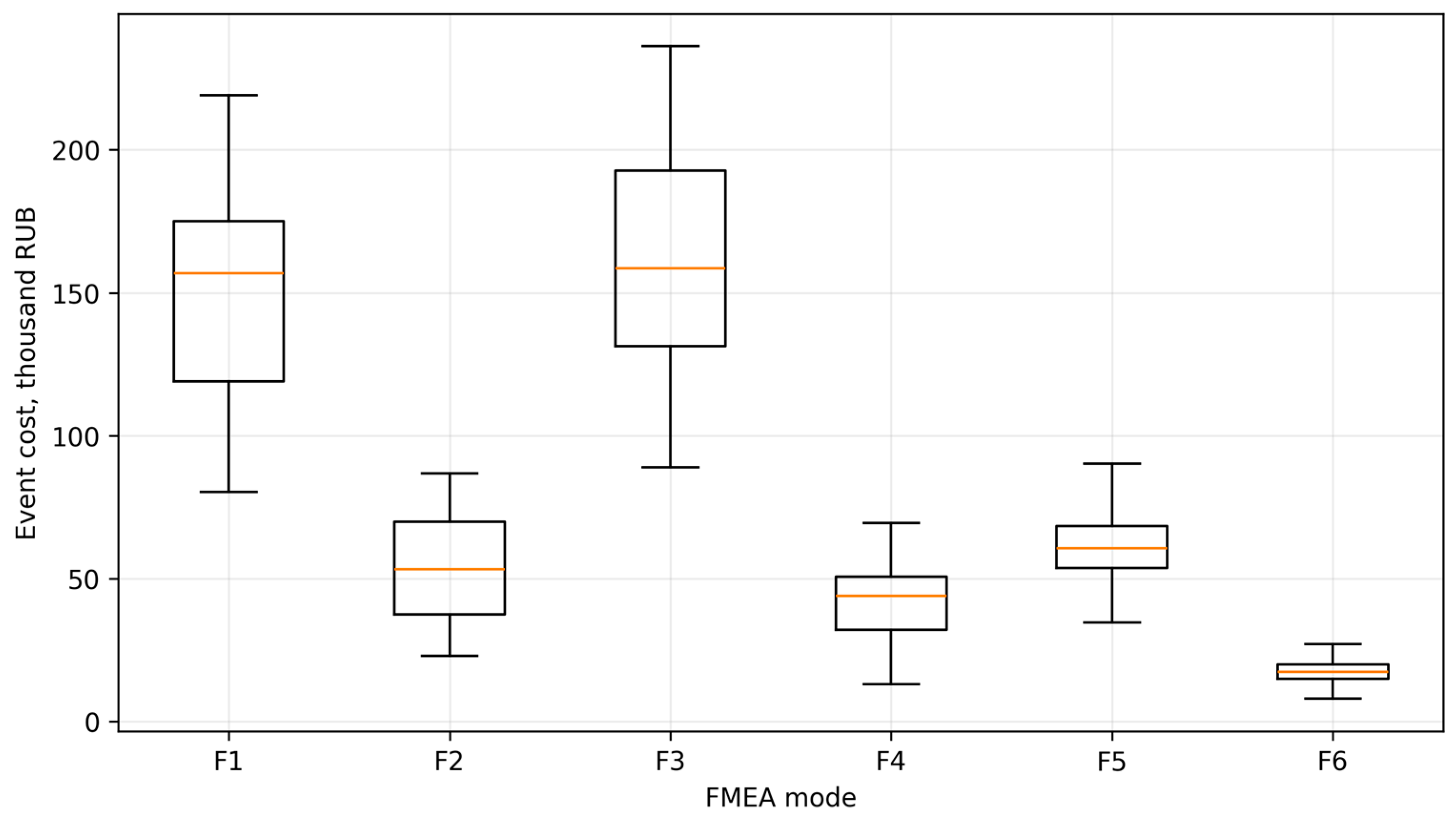
The distribution of the cost of events by failure and regulatory groups is shown in Figure 13.
Figure 13 shows a right-skewed event-cost distribution: median values do not represent the upper tail of expensive repairs and downtime. In the LCC calculation, a small number of high-voltage failures can therefore contribute as much as numerous low-cost scheduled interventions.
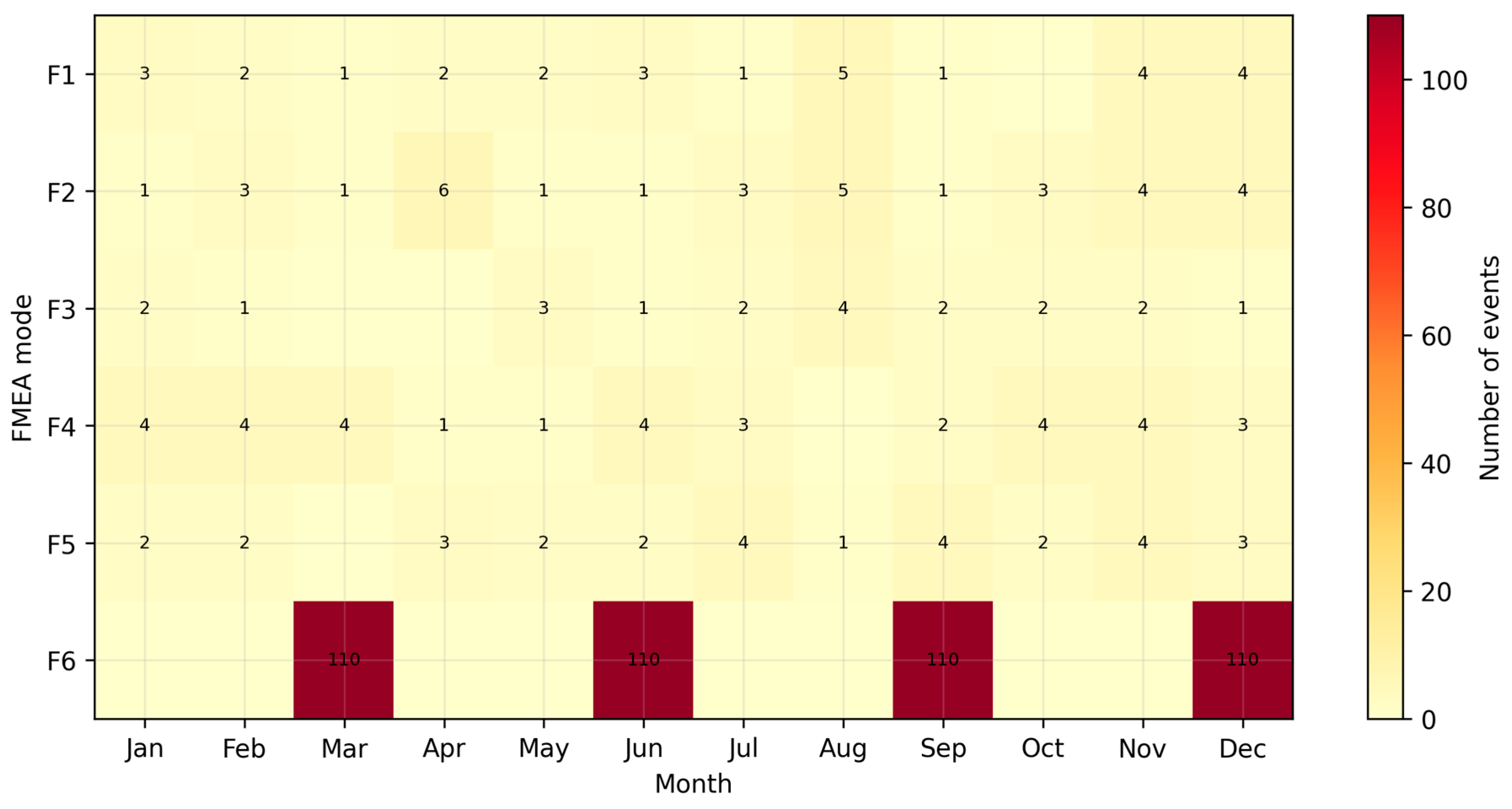
To analyze the seasonal concentration of events, a heat map of the month × event group is constructed, as shown in Figure 14.
Figure 14 shows seasonal clustering, particularly for thermal derating and auxiliary-system events. B2 implementation should therefore include pre-season inspection of heating and cooling circuits, BMS logs, high-voltage insulation, and derating settings.

3.7. LCC: Absolute Decomposition of Life-Cycle Cost

To address the lack of normalized results, Table 13 shows the absolute decomposition of LCC in RUB/km by key components.
Table 13 shows that the principal difference between B1 and B2 is the annualized battery replacement component. B2 increases diagnostic expenditure but reduces the replacement equivalent; the economic effect therefore depends on battery cost, diagnostic cost, the admissible service-life horizon, and controlled risk. Totals were calculated from unrounded components and may differ by 0.001 RUB/km from the sum of the displayed rounded values.
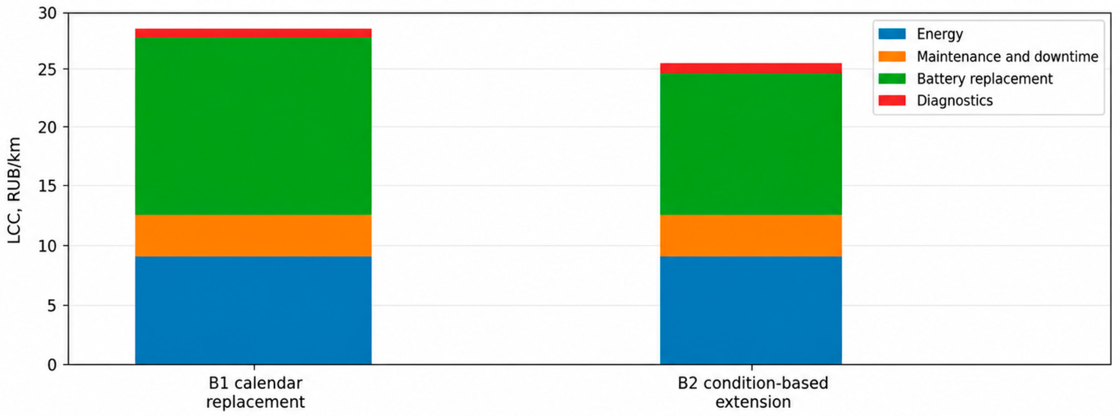
Figure 15 shows the absolute LCC decomposition for B1 and B2.
Figure 15 shows that energy costs are a significant, but not dominant, source of difference between B1/B2 strategies. The main controllable component is the lifespan of the battery kit. Therefore, the economic viability of B2 depends on the reliability of the diagnostic barriers and on the actual cost of battery replacement.

3.8. ELC: Stage Structure of Life-Cycle Emissions

For environmental interpretation, Table 14 shows the stage structure of the ELC: operational electricity, maintenance and repair materials, and battery-conditioned embedded contribution.
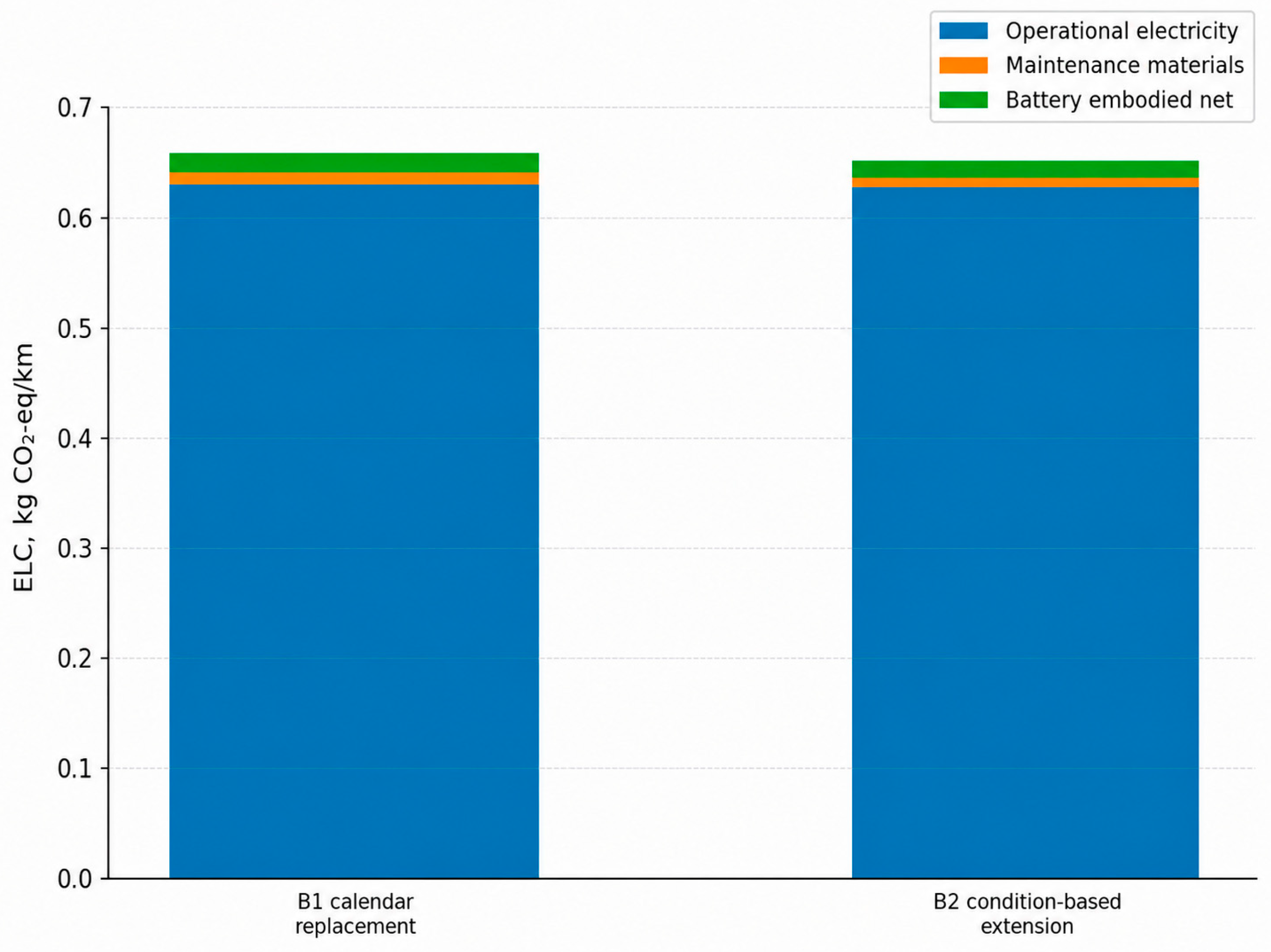
Table 14 shows that operational electricity contributes 0.6419 kg CO2-eq/km, or approximately 96.6% of baseline B1 emissions. Extending battery life reduces the battery-related contribution from 0.0226 to 0.0174 kg CO2-eq/km, while total ELC changes from 0.6646 to 0.6594 kg CO2-eq/km, corresponding to 0.7824%. Totals are based on unrounded components. Table 15 uses alternative network and waste processing scenarios to test the direction and magnitude of output.
Table 15 confirms that the absolute B1–B2 difference remains dominated by the avoided battery-production burden, while the relative benefit depends on the denominator formed by operational electricity. Under the cleaner-grid scenario, the relative ELC reduction increases to 1.59%; under the carbon-intensive scenario, it decreases to 0.56%. Varying the recycling credit from 0% to 20% changes the relative reduction only from 0.87% to 0.70%, so the main conclusion is more sensitive to the grid factor than to the assumed recycling credit.
The stage structure of the ELC is shown in Figure 16.
Figure 16 visually confirms the dominance of the operation stage. In practice, this means that in order to reduce the ELC, the operator needs to work not only with the battery strategy, but also with energy: recuperation, HVAC, driving modes, the schedule of autonomous sections, and the regional EFgrid coefficient.

3.9. Risk, RPN, and Effect of the B2 Diagnostic Strategy

Figure 17 compares the event-informed B1 RPN values with the illustrative B2 values obtained from the control assumptions in Table 12. B2 is considered acceptable only when the specified diagnostics and preventive actions are actually implemented.
Figure 17 shows that the modelled RPN decreases for all F1–F5 modes, but the mechanism differs by mode. F1 benefits from both lower occurrence and improved detection; F2 and F4 are reduced mainly through preventive thermal and high-voltage controls; F3 and F5 are reduced mainly through earlier detection. Severity is unchanged because B2 does not alter the consequence of a failure after it occurs.
The failure-event-weighted RPN decreases from 125.368 to 80.389, corresponding to 35.87% (35.9% after rounding). This is a scenario-based risk-control result, not an observed before–after reduction. Its operational validity must be verified after B2 implementation by comparing normalized event rates, detection lead time, downtime, and severity distributions.

3.10. Multi-Criteria Scenario Comparison and Sensitivity

Table 16 compares six predefined combinations of AH intensity and battery strategy using LCC, ELC, and failure-only event-weighted RPN. The final column reports dominance status only within this discrete evaluated set.
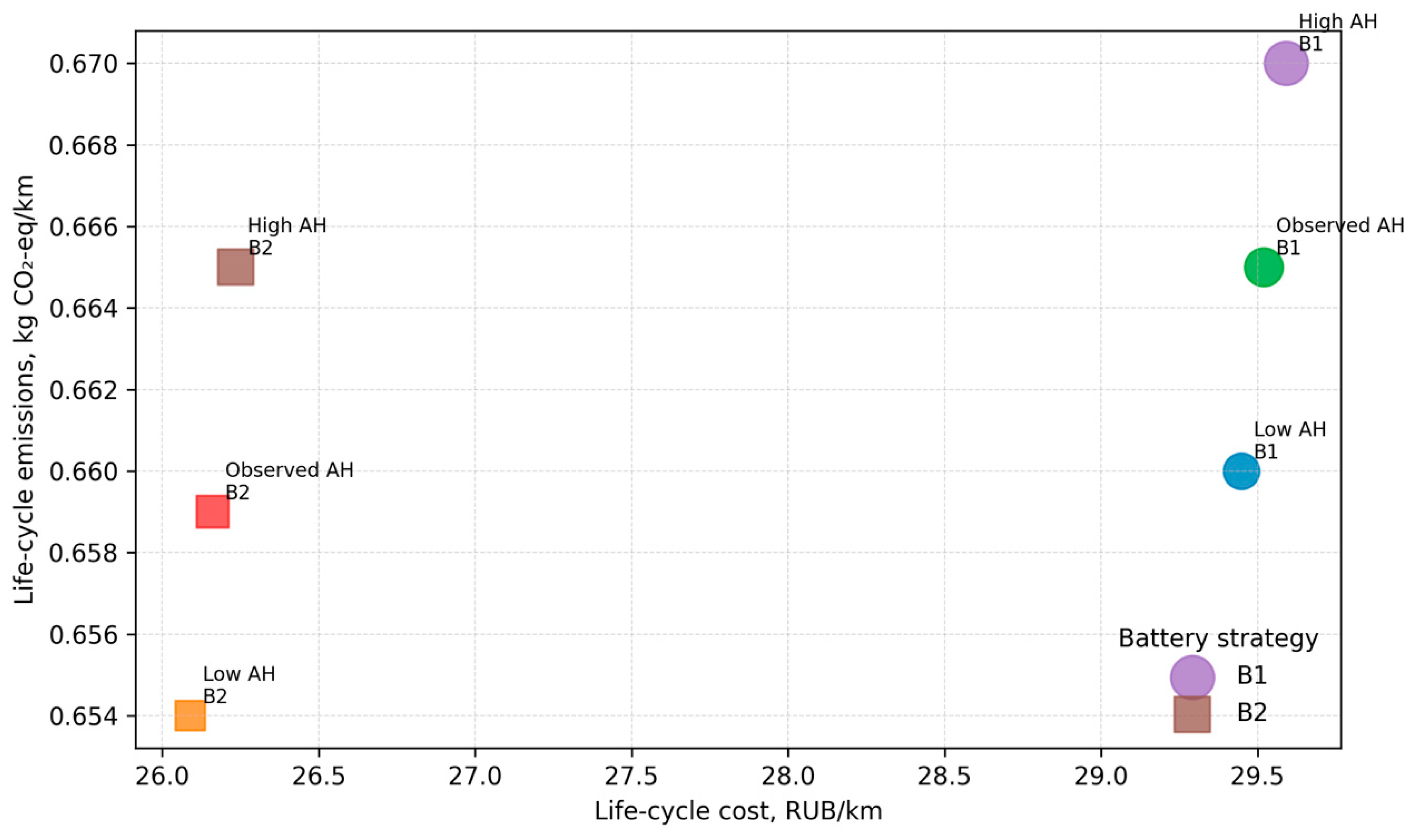
Table 16 shows that low AH–B2 is the only non-dominated member of the six-scenario numerical set because it has the lowest LCC, ELC, and weighted RPN. This result is not automatically transport feasible: a lower AH share may fail to provide the route coverage required on sections without catenary supply. Scenario selection must therefore be performed within a specified service-coverage requirement rather than from the three numerical criteria alone.
Figure 18 visualizes the six scenario positions in LCC–ELC coordinates; marker size represents failure-only event-weighted RPN.
Figure 18 is a discrete scenario map rather than the output of a multi-objective optimizer. B2 shifts each AH-intensity scenario toward lower cost and lower modelled risk, whereas higher AH intensity is associated with a greater energy and emissions burden. The preferred operating policy must therefore be selected from the service-feasible scenarios according to the municipality’s coverage requirement and its acceptable cost, emissions, and risk levels. Table 17 and Table 18 then test the robustness of the economic result to uncertain inputs and battery-life assumptions.
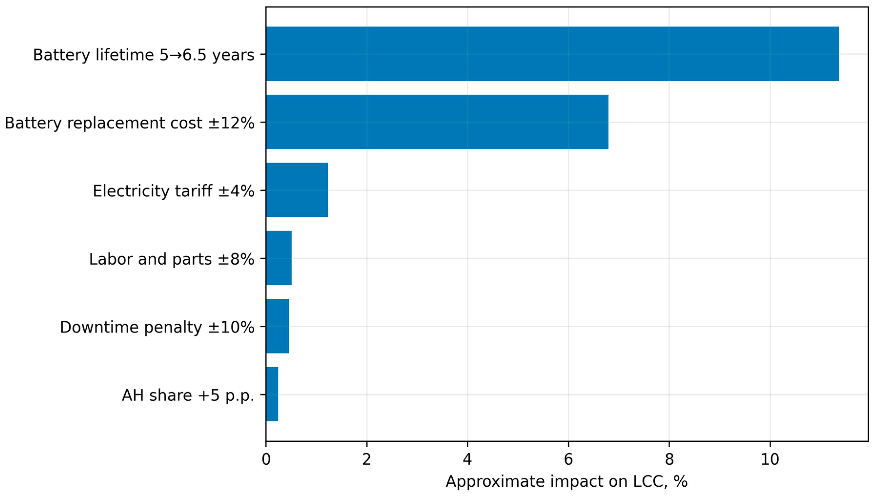
Table 17 shows that the central B2 advantage remains positive over all tested one-way variations. Battery replacement cost produces the widest LCC range, while electricity tariff, labour, downtime, AH share, and diagnostic cost have smaller effects on the relative advantage. The service-life horizon remains the dominant structural assumption and is examined separately in Table 18.
Table 18 shows that the calculated LCC benefit increases monotonically as the assumed battery horizon is extended. However, this mathematical trend does not demonstrate that the longer horizon is technically admissible. The 7.0-year scenario produces the lowest calculated LCC but is not selected as the central case because the available one-year observation period does not validate safe operation at that horizon. The 6.5-year scenario is therefore used as a conditional engineering scenario located between the conservative 5.5–6.0-year extensions and the insufficiently validated 7.0-year case.
Figure 19 summarizes the one-way sensitivity of LCC to the principal battery, tariff, maintenance, downtime, and AH-share assumptions.
Figure 19 and Table 17 and Table 18 show that the B2 result remains positive under the tested tariff, labour, downtime, AH-share, diagnostic cost, and battery cost variations, but its magnitude is strongly dependent on battery replacement cost and the admissible service-life horizon. The B2 saving remains between 10.52% and 12.12% when battery replacement cost varies by ±12%, whereas the horizon analysis ranges from 4.30% at 5.5 years to 13.98% at 7.0 years. The 7.0-year value remains an economic upper scenario and is not accepted without additional ageing validation.
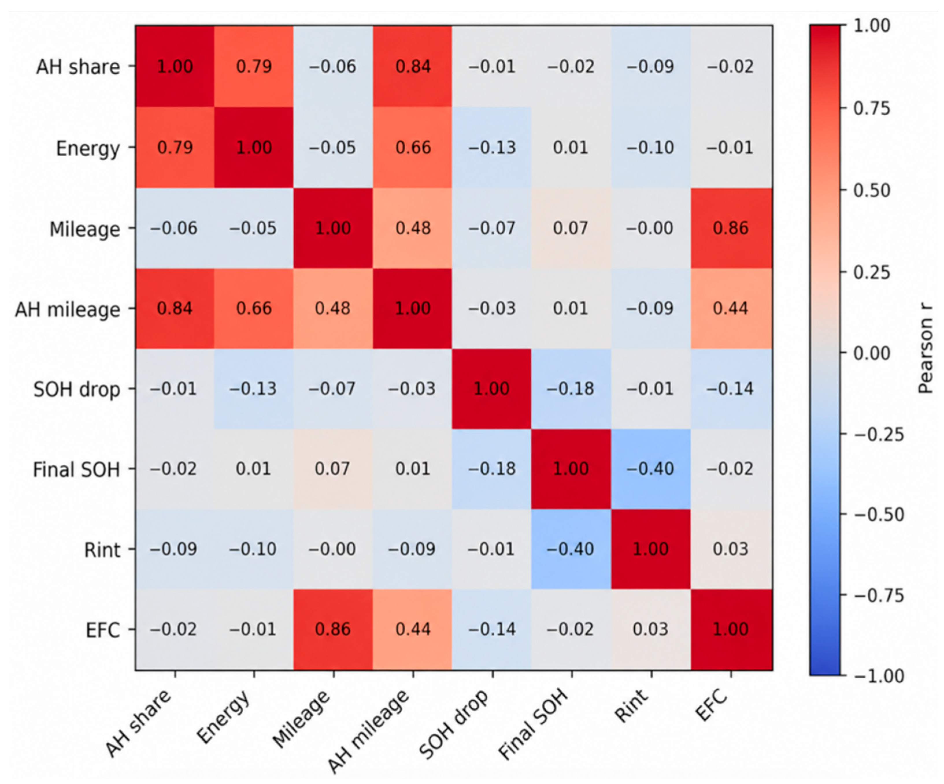
To cross-check the relationships between the key fleet-level indicators, a correlation matrix is constructed, as shown in Figure 20.
Figure 20 shows that pAH is closely related to eavg and AH mileage, whereas SOH drop is more strongly determined by individual resource state and cyclic load. This confirms that the power and resource blocks cannot be reduced to a single pAH variable: a separate SOH/Rint/EFC diagnostic is required for battery policy.

4. Discussion

4.1. Autonomous Operation as a Transport Function and a Controlled Operating Variable

Autonomous operation should be considered both an energy mode and a transport function that provides route flexibility and service continuity beyond the catenary network. The linked database in Table 1 enables the nominal capability of “up to 30 km of autonomous travel” to be replaced by the observed vehicle-day variable pAH. This distinction is important because actual AH mileage is determined by route assignment, shift requirements, temperature, passenger load, and catenary configuration rather than by vehicle capability alone.
Relative to studies focused separately on long-term electric-bus energy monitoring [63], total cost of ownership assessment [64,65], environmental life-cycle assessment [66,67], battery end-of-life and degradation [68,69], or FMEA-based battery risk assessment [70], the present framework advances through observation-level linkage rather than through a new isolated submodel. The same fleet records connect autonomous mileage and seasonal energy demand with SOH, internal resistance, EFC, maintenance events, downtime, LCC, ELC, and failure risk. The methodological advance is cross-domain consistency: B2 is considered acceptable only when its economic benefit is evaluated together with measured battery-condition and explicit risk constraints.
According to Table 4 and Figure 2, the actual average share of autonomous mode was 24.5%, and the total annual mileage of the analyzed fleet reached 6.16 million km. The distribution of pAH across the daily records, shown in Figure 3, demonstrates that the AH mode is used regularly rather than sporadically. Therefore, it cannot be excluded from LCC, ELC, and risk calculations as a secondary mode. On the contrary, autonomous travel should be included in the calculation model as a controllable variable that relates infrastructure constraints, energy efficiency, and battery life.
The energy results confirm a systematic difference between CS and AH operation. Fleet-average net energy consumption is 1.520 kWh/km, while mode-distributed gross energy is 1.521 kWh/km in CS mode and 1.752 kWh/km in AH mode. This difference is consistent with battery conversion losses and the greater influence of temperature and auxiliary demand during autonomous operation.
Autonomous operation is therefore an engineering trade-off between additional energy demand and expanded network functionality. The permissible pAH level should not be selected solely by minimizing kWh/km; it should reflect life-cycle cost, required route coverage, catenary investment alternatives, ESS condition, and operational risk. The proposed LCC–ELC–risk scenario framework supports this decision without representing autonomous operation merely as an energy penalty.

4.2. Energy Model and Seasonal Interpretation of Operational Data

The full-sample fit of the daily-energy model is R2 = 0.860, RMSE = 23.615 kWh/day, and MAPE = 8.119%. In the vehicle-grouped 10-fold validation based on the generated experimental-style dataset, the corresponding out-of-fold values are R2 = 0.842, RMSE = 25.18 kWh/day, and MAPE = 8.74%. The moderate reduction in accuracy is expected because complete annual histories of the test trolleybuses are excluded from coefficient estimation, thereby preventing leakage between repeated vehicle-day records.
As reported in Table 7, the subgroup analysis indicates that seasonal MAPE ranges from 7.92% in autumn to 9.63% in winter. Across daily AH-share classes, MAPE increases from 8.08% in the low-AH group to 9.46% in the high-AH group; route-group errors show a similar increase from 8.11% to 9.32%. This pattern is physically plausible because winter operation and high autonomous mileage combine greater HVAC demand, thermal conditioning, and higher traction-energy variability. The 94.1% empirical coverage of the nominal 95% prediction interval indicates acceptable provisional calibration, although the slight undercoverage in the winter and high-AH groups should be retained in uncertainty propagation to LCC and ELC.
The seasonal pattern of energy consumption presented in Figure 4 shows that temperature is one of the key drivers of change in eavg. At low temperatures, the contribution of HVAC/auxiliary loads increases, and at high temperatures, the load on the cooling systems of the battery and power electronics increases. The three-dimensional surface in Figure 6 clarifies this conclusion: the maximum eavg values are formed not simply by increasing the pAH but by combining a high proportion of autonomous travel and unfavourable temperature conditions. This indicates the need for seasonal calibration of operational standards and route tasks.
The practical interpretation is that the same pAH value is not energetically equivalent in different months of the year. The 10–15 km long autonomous section in summer, winter, and off-season places different loads on the ESS, the traction system, and auxiliary consumers. Therefore, for the dispatching of autonomous trolleybuses, it is advisable to use not only the standard of autonomous mileage but also correction factors that take into account temperature, passenger load, and route profile. This approach improves the accuracy of energy planning and reduces the risk of misestimating the residual life of the battery.
Figure 7 and Figure 8 show that inter-route and inter-depot heterogeneity also have engineering significance. Differences in eavg between routes and depots can be related to the length of autonomous sections, the number of stops, the average speed limit, the quality of the contact network, climatic conditions of storage, and maintenance features. Therefore, the average fleet-level estimate is useful for strategic planning, but operational management requires detailing by routes, depots, and groups of vehicles.

4.3. Economic Interpretation of B2 and the Limits of the Ecological Effect

The LCC results show that the condition-based battery-life extension strategy can be economically significant for an autonomous-range trolleybus fleet. According to Table 13 and Figure 15, the central B2 scenario reduces LCC from 29.52 to 26.16 RUB/km, or by 11.4%. For annual fleet mileage exceeding 6 million km, this difference is operationally material, but it remains conditional on pack-level eligibility and the assumed service-life horizon.
The 11.4% reduction corresponds specifically to the central 6.5-year B2 scenario. It should not be interpreted as a guaranteed fleet-wide saving because B2 eligibility is evaluated separately for each vehicle and limiting battery pack. As shown in Table 18, shorter admissible horizons of 5.5 and 6.0 years reduce LCC by 4.30% and 8.25%, respectively. The calculated 13.98% reduction at seven years is an economic upper scenario only and is not supported as a safe operating recommendation by the present one-year observation period.
The economic mechanism is transparent: B2 lowers the annualized battery replacement component while increasing expenditure on diagnostics and preventive maintenance. It therefore shifts expenditure from capital-intensive replacement toward condition-based maintenance rather than eliminating maintenance costs [69,70].
Environmental outcomes require separate interpretation from LCC. As shown in Table 14 and Figure 16, baseline ELC decreases from 0.6646 to 0.6594 kg CO2-eq/km, or by 0.7824%, because operational electricity accounts for approximately 96.6% of B1 emissions. B2 mainly reduces the embodied battery contribution and cannot substantially change total ELC while the electricity mix and operating energy demand remain unchanged [66,67].
The sensitivity results in Table 15 show how this conclusion changes with the grid mix. When the weighted grid factor is reduced to 0.200 kg CO2-eq/kWh, the relative B2 benefit increases to 1.59% because battery production represents a larger share of the lower total. When the weighted factor rises to 0.600 kg CO2-eq/kWh, the relative benefit decreases to 0.56%. Scaling the monthly factors by ±20% produces a 0.66–0.97% reduction, while changing the recycling credit from 0% to 20% produces a 0.70–0.87% reduction. Thus, the direction of the B2 environmental effect is stable, but its magnitude is modest and grid-dependent.
Therefore, the most effective environmental policy should combine B2 with energy measures: HVAC optimization, improved recovery efficiency, reduced traction chain losses, seasonal AH routing, and the use of low-carbon electricity. In this sense, B2 should be seen as a necessary but not the only element in the decarbonization of the fleet. Its significance lies in the fact that the extension of the ESS service life reduces the material intensity of the life cycle, increases the predictability of the technical condition, and creates a technological basis for further reducing the environmental footprint.

4.4. SOH, Internal Resistance, and EFC for Diagnostics-Guided Battery Service-Life Management

The diagnostic results show that SOH is necessary but insufficient for deciding whether a battery pack can remain in service. According to Table 10 and Figure 9, the fleet-average SOH decreased from 89.98% to 85.94%, whereas internal resistance increased from 14.92 to 15.83 mΩ and the mean accumulated EFC increased from 37.62 to 392.30. At the same time, the persistent between-pack SOH dispersion demonstrates that fleet-average values cannot replace pack-specific screening.
From an electrochemical perspective, the observed trajectory may reflect interacting ageing pathways. Calendar ageing may involve continued interphase growth and loss of cyclable lithium, whereas cyclic ageing may additionally involve active-material degradation, particle cracking, electrolyte decomposition, and impedance growth. Larger DoD, elevated charge or discharge rates, repeated high-temperature exposure, and low-temperature charging can accelerate these processes. These mechanisms are well established, but they cannot be separated uniquely from the available fleet records because chemistry-resolved, C-rate-resolved, and cell-level charging histories were unavailable [71,72,73].
The charging strategy is relevant because the autonomous sections impose additional charge–discharge throughput on the storage system. Nevertheless, the present dataset supports reliable calculation of EFC, mean DoD, temperature exposure, and SOH trajectories but does not provide sufficiently complete high-frequency current data to reconstruct the exact C-rate distribution for every charging event. For this reason, the study does not attribute the measured annual SOH decline to a single charging regime. Instead, EFC, DoD, thermal history, internal resistance, and failure records are used as observable fleet-level stress indicators.
Charging conditions and calendar exposure can alter the diagnostic meaning of the same SOH value. Long residence at high state of charge, elevated charging temperature, high charge or discharge C-rates, deep cycling, frequent fast charging, incomplete preheating, and charging at low cell temperature may accelerate interphase growth, lithium plating, electrolyte degradation, active-material damage, and resistance increase. Calendar ageing also continues during low-mileage or parked periods and depends strongly on time, temperature, and state of charge. Because the fleet exports do not contain complete event-level SOC, current, voltage, charging-temperature, cut-off, and dwell-time histories, B2 eligibility cannot be interpreted as a chemistry-specific lifetime prediction. It is a conservative fleet-management screen that must be supplemented by manufacturer-specific charging limits and periodic capacity and resistance verification.
Electrochemical impedance spectroscopy provides a non-destructive means of separating frequency-dependent resistive and electrochemical responses and is therefore relevant to future pack-level validation of BMS-derived SOH. Recent compact and TinyML-based approaches also indicate that impedance features may be processed on resource-constrained diagnostic hardware. These methods were not used to generate the present SOH results and are discussed only as a future extension of the fleet diagnostic architecture [60,61].
At the cell and electrode-material level, recent in situ and operando studies show how structural transformations, interfacial reactions, ion transport, and degradation can be observed during cycling in two-dimensional-material energy-storage devices [74]. Phase engineering likewise offers routes to modify conductivity, redox activity, ion diffusion, and structural stability [75]. These studies motivate future chemistry-resolved validation but do not provide direct evidence for the commercial packs analyzed here.
The onboard energy-storage system also provides route flexibility, continuity of service beyond the catenary network, and operational resilience. These benefits increase the importance of reliable condition assessment because an incorrectly extended battery lifetime can convert economic savings into derating, loss of autonomous range, or unplanned downtime. Energy storage improves system flexibility and reliability only when degradation and operating constraints are explicitly controlled [76].
Accordingly, the B2 strategy should not be based on one SOH threshold. Its acceptance logic must jointly consider SOH, measured available capacity, internal resistance growth, EFC, DoD, thermal-event history, pack-to-pack dispersion, and the absence of critical battery or high-voltage failure events. This formulation distinguishes a condition-based service-life extension from an unconditional calendar extension.
In operational terms, the B2 decision is conjunctive rather than compensatory. A favourable SOH value cannot compensate for an excessive resistance increase, repeated thermal derating, insufficient autonomous-range reserve, or an unresolved critical failure. Extension is authorized only while all mandatory gates in Table 3 remain satisfied. Any failed gate suspends the extension until corrective action and repeated verification are completed.
The FMEA results support the need for diagnostic gating, but they must be interpreted as an event-informed scenario rather than as an observed post-intervention effect. As shown in Table 12 and Figure 17, the event-weighted RPN decreases from 125.368 to 80.389, or by 35.9%, only under the illustrative B2 occurrence and detection assumptions. The largest modelled reductions occur for F1 and F2, which are directly addressed by SOH-trend, capacity, resistance, temperature, and derating controls. The smaller reductions for F3-F5 show that preventive regulations for power electronics, HV insulation, control systems, and auxiliary subsystems remain necessary.

4.5. Multi-Criteria Scenario Comparison and Managerial Interpretation

The analysis in Table 16 and Figure 18 is a comparison of six predefined scenarios, not a continuous multi-objective optimization. Low AH–B2 is numerically non-dominated within this set, but a low-AH policy may be infeasible when autonomous operation is required to maintain route coverage beyond the catenary network. The relevant managerial choice is therefore the best service-feasible scenario, not an unconstrained numerical minimum.
B2 improves the LCC and modelled risk position at each evaluated AH-intensity level, while its influence on ELC remains modest because operational electricity dominates the environmental total. This separation is useful for management: battery diagnostics and replacement policy primarily affect LCC and risk, whereas grid carbon intensity, HVAC demand, recuperation, and route operation primarily affect ELC.
The sensitivity analysis presented in Table 17 and Figure 19 shows that LCC is most affected by battery replacement cost and the admissible battery service-life horizon. Electricity tariff, labour, downtime, AH share, and diagnostic cost produce smaller changes in the relative B2 advantage. This gives the operator a specific management-priority map: a higher battery-replacement cost strengthens the economic case for B2, whereas inadequate diagnostics, unplanned downtime, or a shorter admissible horizon reduce the benefit. Therefore, B2 requires full integration of diagnostics into the maintenance-planning system rather than formal SOH monitoring alone.
The correlation matrix in Figure 20 complements the scenario comparison by showing the relationships among pAH, eavg, SOH, Rint, EFC, and mileage. The main operational implication is that autonomous mileage, energy efficiency, and ESS condition form an interconnected system. Fleet management should therefore integrate daily operating logs, energy telemetry, battery diagnostics, and failure events within one analytical environment.

4.6. Limitations and Directions for Further Research

First, external validity is limited by the single-city, single-operator, and 12-month study design. Climate, topography, stop density, route topology, catenary conditions, electricity mix, maintenance practices, and procurement prices can change the absolute LCC, ELC, energy, and failure results. The framework is transferable, but the numerical thresholds and outcomes require recalibration before application to another fleet.
Second, the operator supplied anonymized exports rather than the original onboard databases with complete calibration documentation for every measurement channel. Sensor-level measurement uncertainty could therefore not be reconstructed for all 40,150 vehicle-day records. The study reports record-quality categories, empirical ranges, cross-vehicle variability, and model error instead of assigning unsupported retrospective instrument tolerances.
Third, this study is observational. Associations among pAH, temperature, energy consumption, SOH, resistance, EFC, and failures remain vulnerable to residual confounding by route allocation, driver behaviour, passenger load, maintenance timing, charging practice, and unrecorded hardware conditions. The reported associations should not be interpreted as isolated causal effects. Multi-year matched before–after and intercity designs are required for stronger causal inference. The linear specification also does not explicitly resolve nonlinear interactions involving traffic congestion, stop density, road gradient and surface condition, intersection delay, acceleration and braking style, driver-specific behaviour, or catenary-voltage variation.
Fourth, several revision-stage results are illustrative rather than independently observed. The vehicle-grouped validation values use a generated experimental-style dataset, the B2 changes in FMEA occurrence and detection are ex ante control effect assumptions, and the alternative LCC and ELC sensitivity cases are scenario inputs. These values demonstrate the calculation workflow.
Fifth, the electrochemical resolution of the battery data is limited. The fleet exports contain SOH, available capacity, internal resistance, EFC, DoD, temperature, and thermal-event indicators, but not complete cell-level current and voltage trajectories, exact C-rate distributions, charging-cut-off histories, chemistry-resolved pack metadata, or EIS and operando spectra. The analysis therefore supports fleet-level condition monitoring but does not identify individual electrochemical ageing mechanisms. Charging-regime and calendar-ageing effects are therefore represented only indirectly through battery age, EFC, DoD, thermal history, SOH, internal resistance, and observed failure records.
Sixth, B2 had not been implemented as a controlled fleet intervention during the observation period. The 6.5-year battery horizon, diagnostic thresholds, and 35.9% modelled RPN reduction are conditional engineering scenarios rather than verified post-implementation outcomes. Their validation requires repeated eligibility reviews and a multi-year comparison of matched B1 and B2 vehicles, including withdrawals, false alarms, missed detections, and unplanned downtime. The deterministic eligibility rule is not a probability-calibrated decision model and does not quantify threshold uncertainty, dependence among diagnostic indicators, or the probability of safe operation over the proposed extension horizon.
Seventh, the functional unit is one vehicle-kilometre. Passenger-kilometres, occupancy-adjusted transport work, service regularity, catenary capital expenditure, and the economic value of newly served areas were not monetized. Moreover, the multi-criteria analysis evaluates six predefined scenarios rather than searching a continuous decision space. Future work should include service-quality and infrastructure constraints and compare only transport-equivalent alternatives.
These limitations define the evidential boundary of the study. The present contribution is a traceable fleet-level workflow and an internally consistent case analysis, not universal battery thresholds or a validated post-intervention claim. The next stage should combine verified record-level data, manufacturer-specific diagnostic limits, external fleet validation, and a prospective B2 implementation study.

4.7. Practical Recommendations for the Operator and the Municipal Customer

The operator should record autonomous operation explicitly in the daily logs. Ltotal, LCS, LAH, pAH, route, depot, temperature, passenger load, and abnormal-event indicators are required to link route assignment with energy demand, battery conditions, and failures. Without this granularity, fleet-average values cannot support pack-specific B2 decisions.
Energy telemetry should retain total net energy, mode-resolved CS/AH energy, recuperation, HVAC and auxiliary loads, and derating indicators. This structure reduces uncertainty in eCS and eAH and improves transfer of the operational results to LCC and ELC. Data-system modernization can therefore improve routing, maintenance, and ESS replacement decisions alongside hardware modernization.
For B2 implementation, the operator should conduct monthly BMS data screening and a formal eligibility review at least once per quarter. The quarterly review should include BMS-reported SOH, the most recent capacity-referenced SOH, BMS-to-capacity discrepancy, three-month SOH trend, internal resistance growth, pack-to-pack SOH spread, EFC, mean DoD, maximum and minimum cell temperatures, thermal-derating events, autonomous-range reserve, and F1–F5 failure history. A standardized capacity test should be performed at least annually and whenever the BMS SOH approaches 82%, the BMS-to-capacity discrepancy exceeds 1.5 percentage points, or accelerated degradation is detected.
The service-life extension should be approved only when all mandatory gates in Table 3 are satisfied. Failure of one gate should result in temporary suspension of B2, additional diagnostics, route derating, repair, pack replacement, or return to the B1 calendar-replacement policy. Thus, the 6.5-year horizon is not assigned once for the entire fleet but is repeatedly confirmed for each eligible vehicle.
For the municipal customer, an autonomous-range trolleybus is both rolling stock and an element of data-driven transport infrastructure. Its effectiveness depends on purchase cost, rated autonomous range, data quality, diagnostic capability, maintenance rules, and the operator’s ability to manage the battery condition at the fleet level. Fleet expansion should therefore coordinate vehicle procurement, catenary development, telemetry infrastructure, condition-based battery maintenance, and integrated LCC–ELC–risk monitoring. Algorithmic condition-based control studies provide a complementary basis for this data-to-decision architecture [77].

5. Conclusions

This paper presents a fleet-level study of 110 autonomous-range trolleybuses using 40,150 vehicle-day operating records, 40,150 energy records, 3960 pack-month SOH records, and 584 maintenance, failure, and downtime events. Autonomous operation is treated as a measurable mode that influences energy consumption, battery use, life-cycle cost, and operational risk rather than as a nominal vehicle capability.
The daily energy consumption model provides a descriptive performance for the entire sample with a determination coefficient of R2 = 0.860, a root mean square error of RMSE = 23.615 kWh/day, and a mean absolute percentage error of 8.119%. Validation by vehicle group yields R2 = 0.842, RMSE = 25.18 kWh/day, and MAPE = 8.74%, with MAPE for subgroups ranging from 7.92% to 9.63%.
The average SOH of the battery packs decreased from 89.98% to 85.94% over the 12-month observation period, corresponding to a fleet-average decline of 4.04 percentage points. This mean trajectory was accompanied by an increase in internal resistance and EFC, while the persistent between-pack SOH dispersion showed that degradation was not uniform across the fleet. The diagnostic interpretation therefore combines BMS-reported SOH, periodically measured available capacity, internal resistance, EFC, DoD, temperature history, thermal events, and failure records. Because complete chemistry-resolved and C-rate-resolved charging histories were unavailable, the study does not attribute the observed degradation to one electrochemical mechanism. The B2 strategy is consequently formulated as a multiparameter, diagnostic-gated operating policy rather than as a simple calendar-life extension.
In the central 6.5-year scenario, the condition-based battery-life extension strategy reduces LCC from 29.52 to 26.16 RUB/km, corresponding to an 11.4% reduction. The horizon sensitivity analysis shows reductions of 4.30%, 8.25%, 11.38%, and 13.98% for assumed service lives of 5.5, 6.0, 6.5, and 7.0 years, respectively. These values demonstrate the strong dependence of the economic result on the assumed battery horizon but do not independently establish technical admissibility. The 6.5-year horizon is therefore treated as a conditional central scenario, while actual extension is approved pack-by-pack only when all diagnostic gates remain satisfied. The event-weighted RPN for F1–F5 decreases from 125.368 to 80.389, or 35.9%, with the presence and detection of B2; this decrease requires prompt pre- and post-testing.
Baseline ELC decreases from 0.6646 to 0.6594 kg CO2-eq/km, corresponding to 0.7824%. The cleaner-grid scenario increases the relative B2 benefit to 1.59%, whereas the carbon-intensive scenario reduces it to 0.56%. The environmental advantage is therefore directionally stable but modest because operating electricity dominates total emissions and the battery strategy mainly affects the embodied component.
Taken together, this study contributes an observation-linked fleet assessment framework rather than a new standalone battery or energy model. The framework preserves a traceable sequence from vehicle-day operation through pack-month diagnostics and event-level maintenance data to LCC, ELC, and event-weighted RPN. Battery-life extension should only be approved for in-service vehicles whose limiting batteries continue to meet the full set of diagnostic criteria.

Author Contributions

Conceptualization, V.S.T., B.V.M. and N.V.M.; methodology, V.A.G. and T.A.P.; software, M.A.M.; validation, A.S.G. and V.V.T.; formal analysis, V.A.G. and T.A.P.; investigation, A.S.G. and V.V.T.; resources, A.S.G. and V.V.T.; writing—original draft preparation, V.S.T., B.V.M. and N.V.M.; writing—review and editing, V.A.G., M.A.M. and T.A.P.; visualization, M.A.M. All authors have read and agreed to the published version of the manuscript.

Funding

This research received no external funding.

Institutional Review Board Statement

Not applicable.

Informed Consent Statement

Not applicable.

Data Availability Statement

The original contributions presented in this study are included in the article. Further inquiries can be directed to the corresponding author.

Conflicts of Interest

The authors declare no conflicts of interest.

Notation

pAH is the observed share of autonomous mileage in total daily mileage (–);
CS is the contact-network power-supply mode;
AH is the autonomous-operation mode;
eavg, eCS, and eAH are the average net, contact-supply, and autonomous-mode-specific energy values, respectively (kWh/km);
SOH is the battery-pack state of health (%);
Rint is the battery-pack internal resistance (mΩ);
EFC is the number of equivalent full cycles;
DoD is the depth of discharge (%);
LCC is the life-cycle cost (RUB/km);
ELC is the life-cycle emissions (kg CO2-eq/km);
FMEA is failure mode and effects analysis;
RPN is the risk priority number, calculated as severity × occurrence × detection;
F1–F5 are the failure modes included in the fleet-level FMEA;
SM denotes scheduled-maintenance events included in LCC and availability calculations but excluded from weighted RPN.

References

  1. Pietrzak, K.; Pietrzak, O. Environmental effects of electromobility in a sustainable urban public transport. Sustainability 2020, 12, 1052. [Google Scholar] [CrossRef] [Scilit]
  2. Priemus, H.; Nijkamp, P.; Banister, D. Mobility and spatial dynamics: An uneasy relationship. J. Transp. Geogr. 2001, 9, 167–171. [Google Scholar] [CrossRef] [Scilit]
  3. Bos, R.; Temme, R. A Roadmap towards sustainable mobility in Breda. Transp. Res. Procedia 2014, 4, 103–115. [Google Scholar] [CrossRef] [Scilit]
  4. Lindholm, M.; Behrends, S. Challenges in urban freight transport planning—A review in the Baltic Sea Region. J. Transp. Geogr. 2012, 22, 129–136. [Google Scholar] [CrossRef] [Scilit]
  5. Newman, P.W.G.; Kenworthy, J.R. The land use-transport connection: An overview. Land Use Policy 1996, 13, 1–22. [Google Scholar] [CrossRef] [Scilit]
  6. Broto, V.C. Energy landscapes and urban trajectories towards sustainability. Energy Policy 2017, 108, 755–764. [Google Scholar] [CrossRef] [Scilit]
  7. Martyushev, N.V.; Malozyomov, B.V.; Demin, A.Y.; Pogrebnoy, A.V.; Kurdyumov, G.E.; Kondratiev, V.V.; Karlina, A.I. Comparative Assessment of the Reliability of Non-Recoverable Subsystems of Mining Electronic Equipment Using Various Computational Methods. Mathematics 2026, 14, 723. [Google Scholar] [CrossRef] [Scilit]
  8. Un-Habitat. Planning and Design for Sustainable Urban Mobility; Un-Habitat: Nairobi, Kenya, 2013. [Google Scholar]
  9. Sarybayev, Y.Y.; Balgayev, D.Y.; Tkachenko, D.Y.; Martyushev, N.V.; Malozyomov, B.V.; Beisenov, B.S.; Sorokova, S.N. Reliability-Oriented Modeling of Bellows Compensators: A Comparative PDE-Based Study Using Finite Difference and Finite Element Methods. Mathematics 2025, 13, 3452. [Google Scholar] [CrossRef] [Scilit]
  10. Malozyomov, B.V.; Khekert, E.V.; Martyushev, N.V.; Konyukhov, V.Y.; Chetverikova, V.V.; Golik, V.I.; Tynchenko, V.S. Improving the Reliability of the Protection of Electric Transport Networks. World Electr. Veh. J. 2025, 16, 477. [Google Scholar] [CrossRef] [Scilit]
  11. European Commission. Action Plan on Urban Mobility; COM(2009) 490 Final; European Commission: Brussels, Belgium, 2009; pp. 1–13. [Google Scholar]
  12. European Commission. A European Strategy for Low-Emission Mobility; European Commission: Brussels, Belgium, 2016. [Google Scholar]
  13. Gärling, T.; Schuitema, G. Travel demand management targeting reduced private car use: Effectiveness, public acceptability and political feasibility. J. Soc. Issues 2007, 63, 139–153. [Google Scholar] [CrossRef] [Scilit]
  14. Zadkov, D.A.; Martyushev, N.V.; Malozyomov, B.V.; Demin, A.Y.; Pogrebnoy, A.V.; Kuleshova, E.E.; Valuev, D.V. Mathematical Modeling of Operational Reliability of Mine Lifting Equipment Based on Censored Data. Mathematics 2026, 14, 716. [Google Scholar] [CrossRef] [Scilit]
  15. Song, Y.; Preston, J.; Ogilvie, D. New walking and cycling infrastructure and modal shift in the UK: A quasi-experimental panel study. Transp. Res. Part A Policy Pract. 2017, 95, 320–333. [Google Scholar] [CrossRef] [Scilit] [PubMed]
  16. Welcome to 2030: The Mega-Trends. Available online: https://ec.europa.eu/assets/epsc/pages/espas/chapter1.html (accessed on 25 October 2020).
  17. Bartłomiejczyk, M.; Kołacz, R. The reduction of auxiliaries power demand: The challenge for electromobility in public transportation. J. Clean. Prod. 2020, 252, 119776. [Google Scholar] [CrossRef] [Scilit]
  18. Malmö Stad. Sustainable Urban Mobility Plan: Creating a More Accessible Malmö; Malmö Stad: Malmö, Sweden, 2016. [Google Scholar]
  19. Nussipali, R.; Martyushev, N.V.; Malozyomov, B.V.; Tynchenko, V.S.; Kukartsev, V.A.; Tynchenko, Y.A.; Panfilova, T.A. Adaptive Corridor-Based Control of a Lithium-Ion Battery Energy Storage System for Wind-Turbine Power Stabilisation and Reliability Improvement in Industrial Microgrids. Electricity 2026, 7, 56. [Google Scholar] [CrossRef] [Scilit]
  20. World Economic Forum. A Report on the Global Agenda Council on Competitiveness; World Economic Forum: Cologny, Switzerland, 2014; p. 60. [Google Scholar]
  21. Maraš, V.; Bugarinović, M.; Anoyrkati, E.; Avarello, A. Megatrends, a way to identify the future transport challenges. Intell. Syst. Comput. 2019, 879, 34–41. [Google Scholar]
  22. European Commission. Public Transport Trends; Executive Summary; European Commission: Brussels, Belgium, 2019. [Google Scholar]
  23. Urbanek, A. Data-Driven Transport Policy in Cities: A Literature Review and Implications for Future Developments. In Integration as Solution for Advanced Smart Urban Transport Systems, Proceedings of the 15th Scientific and Technical Conference “Transport Systems. Theory & Practice”, Katowice, Poland, 20–21 September 2018; Sierpiński, G., Ed.; Springer: Berlin/Heidelberg, Germany, 2019; pp. 61–74. [Google Scholar]
  24. Pryalukhin, A.F.; Martyushev, N.V.; Malozyomov, B.V.; Demin, A.Y.; Pogrebnoy, A.V.; Kuleshova, E.E.; Valuev, D.V. Statistical Modeling and Forecasting of Operational Reliability of Induction Motors of Mining Dump Trucks. Mathematics 2026, 14, 706. [Google Scholar] [CrossRef] [Scilit]
  25. Liebl, F.; Schwarz, J.O. Normality of the future: Trend diagnosis for strategic foresight. Futures 2010, 42, 313–327. [Google Scholar] [CrossRef] [Scilit]
  26. United Nations. Paris Agreement; United Nations: New York, NY, USA, 2015. [Google Scholar]
  27. Fuhr, H.; Hickmann, T.; Kern, K. The role of cities in multi-level climate governance: Local climate policies and the 1.5 °C target. Curr. Opin. Environ. Sustain. 2018, 30, 1–6. [Google Scholar] [CrossRef] [Scilit]
  28. National Travel Survey. Stat. Release 2017; National Travel Survey: London, UK, 2018.
  29. Lozzi, G.; Rodrigues, M.; Marcucci, E.; Teoh, T.; Gatta, V.; Pacelli, V. COVID-19 and Urban Mobility: Impacts and Perspectives; European Parliament: Brussels, Belgium, 2020. [Google Scholar]
  30. Hebel, K. Travel Behaviour Survey of Urban Inhabitants Conducted in Polish Cities. The Theoretical and Practical Aspects; Wyd. Fundacji Rozwoju Uniwersytetu Gdańskiego: Gdańsk, Poland, 2013. (In Polish) [Google Scholar]
  31. Trinh, T.A.; Linh Le, T.P. Investigating Proenvironmental Behavior: The Case of Commuting Mode Choice. In Proceedings of the IOP Conference Series: Earth and Environmental Science, Banda Aceh, Indonesia, 26–27 September 2018; Volume 143. [Google Scholar] [CrossRef] [Scilit]
  32. Ardila-Gomez, A.; Ortegón-Sánchez, A. Sustainable Urban Transport Financing from the Sidewalk to the Subway: Capital, Operations, and Maintenance Financing; World Bank Group: Washington, DC, USA, 2015. [Google Scholar]
  33. Bucsky, P. Modal share changes due to COVID-19: The case of Budapest. Transp. Res. Interdiscip. Perspect. 2020, 8, 100141. [Google Scholar] [CrossRef] [Scilit] [PubMed]
  34. Smith, K. UITP Projects €40bn Hit for European Public Transport in 2020. Int. Railw. J. 2020. Available online: https://www.railjournal.com/financial/uitp-projects-e40bn-hit-for-european-public-transport-in-2020/ (accessed on 1 June 2026). [CrossRef] [Scilit]
  35. Issametova, M.; Martyushev, N.V.; Malozyomov, B.V.; Demin, A.Y.; Pogrebnoy, A.V.; Kuleshova, E.E.; Valuev, D.V. Reliability in Robotics and Intelligent Systems: Mathematical Modeling and Algorithmic Innovations. Mathematics 2026, 14, 580. [Google Scholar] [CrossRef] [Scilit]
  36. Civity Management Consultant. Verkehrswende: Aufgehoben Oder Aufgeschoben? Corona-Szenarien für den ÖPNV; Executive Summary; Civity Management Consultant: Warsaw, Poland, 2020. [Google Scholar]
  37. Wołek, M.; Wyszomirski, O.; Hebel, K.; Grzelec, K.; Połom, M.; Bartłomiejczyk, M.; Pudło, J.; Czermański, E.; Kołodziejski, H.; Debicka, O.; et al. The Trolleybus as an Urban Means of Transport in the Light of the Trolley Project; Wolek, M., Wyszomirski, O., Eds.; University of Gdansk Press: Sopot, Poland, 2013. [Google Scholar]
  38. Martyushev, N.V.; Malozyomov, B.V.; Gladkikh, V.A.; Demin, A.Y.; Pogrebnoy, A.V.; Kuleshova, E.E.; Karlina, Y.I. Adaptive Iterative Algorithm for Optimizing the Load Profile of Charging Stations with Restrictions on the State of Charge of the Battery of Mining Dump Trucks. Mathematics 2025, 13, 3964. [Google Scholar] [CrossRef] [Scilit]
  39. Penina, N.; Turygin, Y.V.; Racek, V. Comparative analysis of different types of hybrid electric vehicles. In Proceedings of the 13th International Symposium on Mechatronics, Mechatronika, Teplice, Slovakia, 2–4 June 2010. [Google Scholar]
  40. Fayyad, S.M.; Abuzalata, M.; Abu-Ein, S. Optimization of the Electrical Motor Generator in Hybrid Automobiles; University of Waterloo: Waterloo, Belgium, 2012; Volume 5. [Google Scholar]
  41. Gay, S.E.; Gao, H.; Ehsani, M. Fuel cell hybrid drive train configurations and motor drive selection. In Proceedings of the IEEE Vehicular Technology Conference, Vancouver, BC, Canada, 24–28 September 2002; Volume 56. [Google Scholar]
  42. Ruiz, V.; Di Persio, F. Standards for the Performance and Durability Assessment of Electric Vehicle Batteries; JRC Technical Reports; Publications Office of the European Union: Brussels, Belgium, 2018. [Google Scholar]
  43. Teegavarapu, S.; Summers, J.D. Case Study Method for Design Research: A Justification. In Proceedings of the ASME 2008 International Design Engineering Technical Conferences & Computers and Information in Engineering Conference, New York, NY, USA, 3–6 August 2008; pp. 1–9. [Google Scholar]
  44. Yin, R.K. Case Study Research: Design and Methods; Applied Social Research Methods Series; Sage: Thousand Oaks, CA, USA, 2003; Volume 5. [Google Scholar]
  45. Koniak, M.; Czerepicki, A.; Tomczuk, P.; Samsul, B. Simulation of the Battery Pack Exploitation Based on Real Measurement Data of Applied Chemical Cells. In Proceedings of the MATEC Web of Conferences, Chongqing, China, 15–17 June 2016; Volume 77. [Google Scholar]
  46. Hong, J.; Tang, M.; Wu, Z.; Miao, Z.; Qiping, G. The evolution of patterns within embodied energy flows in the Chinese economy: A multi-regional-based complex network approach. Sustain. Cities Soc. 2019, 47, 101500. [Google Scholar] [CrossRef] [Scilit]
  47. Eisenhardt, K.M. Theory building from cases: Opportunities and challenges. Acad. Manag. J. 2007, 50, 25–32. [Google Scholar] [CrossRef] [Scilit]
  48. Steenhuis, H.-J.; de Bruijn, E.J. Building Theories from Case Study Research: The Progressive Case Study. OM in the new world uncertainties. In Proceedings of the 17th Annual Conference of POMS, Boston, MA, USA, 28 April–1 May 2006; pp. 1–13. [Google Scholar]
  49. Lowe, M.; Tokuoka, S.; Trigg, T.; Gereffi, G. Lithium-Ion Batteries for Electric Vehicles; NREL: Golden, CO, USA, 2013; pp. 1–13. [CrossRef]
  50. Fleurbaey, K.; Omar, N.; Baghdadi, M.; El Timmermans, J.-M.; Van Mierlo, J. Analysis of hybrid rechargeable energy storage systems in series plug-in hybrid electric vehicles based on simulations. Energy Power Eng. 2014, 6, 195–211. [Google Scholar] [CrossRef]
  51. Shkarupa, O.; Vlasenko, D.; Vesperis, S.; Treus, A.; Juhaszova, Z. Strategic Management for Sustainable Decisions in Business: A Case of Greening the Transport Companies. Probl. Perspect. Manag. 2021, 19, 314–326. [Google Scholar] [CrossRef] [Scilit]
  52. Miles, R. Complexity, representation and practice: Case study as method and methodology. Issues Educ. Res. 2015, 25, 309–318. [Google Scholar]
  53. Flyvbjerg, B. Case study. In The Sage Handbook of Qualitative Research; SAGE Publications Ltd.: Thousand Oaks, CA, USA, 2014; pp. 301–316a. [Google Scholar]
  54. Wołek, M.; Wolański, M.; Bartłomiejczyk, M.; Wyszomirski, O.; Grzelec, K.; Hebel, K. Ensuring sustainable development of urban public transport: A case study of the trolleybus system in Gdynia and Sopot (Poland). J. Clean. Prod. 2020, 279, 123807. [Google Scholar] [CrossRef] [Scilit]
  55. Sierpiński, G.; Staniek, M.; Kłos, M.J. Decision making support for local authorities choosing the method for siting of in-city ev charging stations. Energies 2020, 13, 4682. [Google Scholar] [CrossRef] [Scilit]
  56. Shishkin, P.V.; Malozyomov, B.V.; Martyushev, N.V.; Kondratiev, V.V.; Dorofeev, E.M.; Kononenko, R.V.; Vit’kina, G.Y. Optimization of Energy Balance and Powertrain for Electric Mining Dump Trucks in Coal Mine Reclamation Operations. World Electr. Veh. J. 2025, 16, 601. [Google Scholar] [CrossRef] [Scilit]
  57. Mathieu, L. Electric Buses Arrive on Time—Marketplace, Economic, Technology, Environmental and Policy Perspectives for Fully Electric Buses in the EU; European Federation for Transport and Environment: Brussels, Belgium, 2018. [Google Scholar]
  58. Lajunen, A. Lifecycle costs and charging requirements of electric buses with different charging methods. J. Clean. Prod. 2018, 172, 56–67. [Google Scholar] [CrossRef] [Scilit]
  59. Bartłomiejczyk, M. Praktyczna aplikacja In Motion Charging w Gdyni: Trolejbusy w obsłudze linii autobusowych. Autobusy Tech. Eksploat. Syst. Transp. 2016, 7–8, 58–64. [Google Scholar]
  60. Lazanas, A.C.; Prodromidis, M.I. Electrochemical Impedance Spectroscopy—A Tutorial. ACS Meas. Sci. Au 2023, 3, 162–193. [Google Scholar] [CrossRef] [Scilit] [PubMed]
  61. Giazitzis, S.; Isse, A.A.; Blasuttigh, N.; Massi Pavan, A.; Raimondo, D.M.; Badha, S.; Rosetti, F.; Ogliari, E. TinyML Models for SoH Estimation of Lithium-Ion Batteries Based on Electrochemical Impedance Spectroscopy. J. Power Sources 2025, 653, 237568. [Google Scholar] [CrossRef] [Scilit]
  62. Wołek, M.; Hebel, K. Strategic planning of the development of trolleybus transportation within the cities of Poland. In Smart and Green Solutions for Transport Systems, Proceedings of the 16th Scientific and Technical Conference “Transport Systems. Theory and Practice 2019”, Katowice, Poland, 16–18 September 2019; Sierpinski, G., Ed.; Springer Nature: Cham, Switzerland, 2020. [Google Scholar]
  63. Klaproth, T.; Berendes, E.; Lehmann, T.; Kratzing, R.; Ufert, M. Empirical Energy Consumption Estimation and Battery Operation Analysis from Long-Term Monitoring of an Urban Electric Bus Fleet. World Electr. Veh. J. 2025, 16, 419. [Google Scholar] [CrossRef] [Scilit]
  64. Grauers, A.; Borén, S.; Enerbäck, O. Total Cost of Ownership Model and Significant Cost Parameters for the Design of Electric Bus Systems. Energies 2020, 13, 3262. [Google Scholar] [CrossRef] [Scilit]
  65. Jefferies, D.; Göhlich, D. A Comprehensive TCO Evaluation Method for Electric Bus Systems Based on Discrete-Event Simulation Including Bus Scheduling and Charging Infrastructure Optimisation. World Electr. Veh. J. 2020, 11, 56. [Google Scholar] [CrossRef] [Scilit]
  66. Lubecki, A.; Szczurowski, J.; Zarębska, K. A Comparative Environmental Life Cycle Assessment Study of Hydrogen Fuel, Electricity and Diesel Fuel for Public Buses. Appl. Energy 2023, 350, 121766. [Google Scholar] [CrossRef] [Scilit]
  67. Brambilla, P.C.; Girardi, P. Life Cycle Assessment of Urban Electric Bus: An Application in Italy. Sustainability 2025, 17, 9786. [Google Scholar] [CrossRef] [Scilit]
  68. Canals Casals, L.; Rodríguez, M.; Corchero, C.; Carrillo, R.E. Evaluation of the End-of-Life of Electric Vehicle Batteries According to the State-of-Health. World Electr. Veh. J. 2019, 10, 63. [Google Scholar] [CrossRef] [Scilit]
  69. Edge, J.S.; O’Kane, S.; Prosser, R.; Kirkaldy, N.D.; Patel, A.N.; Hales, A.; Ghosh, A.; Ai, W.; Chen, J.; Yang, J.; et al. Lithium Ion Battery Degradation: What You Need to Know. Phys. Chem. Chem. Phys. 2021, 23, 8200–8221. [Google Scholar] [CrossRef] [Scilit] [PubMed]
  70. Kirana, R.C.; Purwanto, N.A.; Azis, N.A.; Joelianto, E.; Santosa, S.P.; Budiman, B.A.; Nguyen, L.H.; Turnip, A. Failure Assessment in Lithium-Ion Battery Packs in Electric Vehicles Using the Failure Modes and Effects Analysis (FMEA) Approach. J. Mechatron. Electr. Power Veh. Technol. 2023, 14, 94–104. [Google Scholar] [CrossRef] [Scilit]
  71. Vetter, J.; Novák, P.; Wagner, M.R.; Veit, C.; Möller, K.-C.; Besenhard, J.O.; Winter, M.; Wohlfahrt-Mehrens, M.; Vogler, C.; Hammouche, A. Ageing Mechanisms in Lithium-Ion Batteries. J. Power Sources 2005, 147, 269–281. [Google Scholar] [CrossRef] [Scilit]
  72. Keil, P.; Jossen, A. Charging Protocols for Lithium-Ion Batteries and Their Impact on Cycle Life—An Experimental Study with Different 18650 High-Power Cells. J. Energy Storage 2016, 6, 125–141. [Google Scholar] [CrossRef] [Scilit]
  73. Birkl, C.R.; Roberts, M.R.; McTurk, E.; Bruce, P.G.; Howey, D.A. Degradation Diagnostics for Lithium Ion Cells. J. Power Sources 2017, 341, 373–386. [Google Scholar] [CrossRef] [Scilit]
  74. Chandra Mouli, K.V.V.; Mani, D.; Ramachandran, T.; Kumar, Y.A.; Ghosh, A.; Somu, P.; Mangiri, R. A New Era in Energy Storage: In Situ and Operando Characterization of 2D Materials-Based Devices. Mater. Chem. Phys. 2026, 348, 131660. [Google Scholar] [CrossRef] [Scilit]
  75. Mangiri, R.; Reddy, N.P.; Bae, J. Phase Engineering of Nanomaterials: Tailoring Crystal Phases for High-Performance Batteries and Supercapacitors. Micromachines 2025, 16, 1289. [Google Scholar] [CrossRef] [Scilit] [PubMed]
  76. Islam, M.M.; Yu, T.; Giannoccaro, G.; Mi, Y.; La Scala, M.; Rajabi Nasab, M.; Wang, J. Improving Reliability and Stability of Power Systems: A Comprehensive Review on the Role of Energy Storage Systems to Enhance Flexibility. IEEE Access 2024, 12, 152738–152765. [Google Scholar] [CrossRef] [Scilit]
  77. Yelemessov, K.; Baskanbayeva, D.; Sabirova, L.; Martyushev, N.V.; Malozyomov, B.V.; Zhanar, T.; Golik, V.I. Algorithmic Optimal Control of Screw Compressors for Energy-Efficient Operation in Smart Power Systems. Algorithms 2025, 18, 583. [Google Scholar] [CrossRef] [Scilit]
Figure 1. Empirical data workflow linking fleet records, route logs, energy telemetry, SOH diagnostics, maintenance events, and life-cycle decision metrics.
Wevj 17 00377 g001
Figure 2. Monthly fleet mileage and actual autonomous-mode share over the 12-month observation period.
Wevj 17 00377 g002
Figure 3. Distribution of daily autonomous-mode share across 40,150 vehicle-day records.
Wevj 17 00377 g003
Figure 4. Seasonal specific energy by traction mode and monthly ambient temperature.
Wevj 17 00377 g004
Figure 5. Validation and residual diagnostics of the daily-energy model: (a) measured versus predicted daily energy with the 1:1 line; (b) residuals versus fitted values; (c) quantile–quantile plot of standardized residuals; and (d) subgroup MAPE by season, daily AH-share class, and route-AH tertile.
Wevj 17 00377 g005
Figure 6. Three-dimensional fitted empirical energy response surface as a function of autonomous-mode share and ambient temperature.
Wevj 17 00377 g006
Figure 7. Route-level relation between autonomous-mode share and annual mean specific energy.
Wevj 17 00377 g007
Figure 8. Inter-vehicle heterogeneity of annual mean specific energy grouped by depot.
Wevj 17 00377 g008
Figure 9. Battery SOH and internal-resistance dynamics over the 12-month observation period.
Wevj 17 00377 g009
Figure 10. Three-dimensional nonlinear fitted SOH response surface showing the combined effect of equivalent full cycles and maximum cell temperature.
Wevj 17 00377 g010
Figure 11. SOH versus internal resistance with colour-coded equivalent full cycles.
Wevj 17 00377 g011
Figure 12. Failure and scheduled-maintenance event groups with total downtime.
Wevj 17 00377 g012
Figure 13. Distribution of maintenance, failure, and downtime cost by event group.
Wevj 17 00377 g013
Figure 14. Monthly concentration of failure and scheduled-maintenance events by event group.
Wevj 17 00377 g014
Figure 15. Life-cycle cost decomposition for the calendar-replacement strategy and the condition-based battery-life extension strategy.
Wevj 17 00377 g015
Figure 16. Life-cycle emissions decomposition for the calendar-replacement strategy and the condition-based battery-life extension strategy.
Wevj 17 00377 g016
Figure 17. FMEA risk priority numbers for B1 and B2 across five failure modes.
Wevj 17 00377 g017
Figure 18. Cost–emission–risk map for six discrete AH-intensity and battery-strategy scenarios using failure-only event-weighted RPN.
Wevj 17 00377 g018
Figure 19. Sensitivity of life-cycle cost to battery, tariff, downtime, maintenance, and AH-share assumptions.
Wevj 17 00377 g019
Figure 20. Correlation matrix of fleet-level mileage, energy, SOH, resistance, and cycling indicators.
Wevj 17 00377 g020
Table 1. Composition of the linked empirical database used in the fleet-level analysis.
Data BlockVolumeKey FieldsUsage in the Article
02_Fleet_registry110vehicle_id_hash, depot, capacity, odometerFleet definition, mileage normalization, and completeness check
03_Daily_route_logs40,150date, vehicle, route, total_km, CS_km, AH_km, temperaturepAH, daily mileage, seasonality, routing
04_Energy_telemetry40,150total_energy, CS_energy, AH_energy, regen, HVACeavg, eCS, eAH, energy-model validation
05_Battery_SOH3960SOH, capacity, internal resistance, EFC, temperatureESS condition, B2 diagnostics, and degradation assessment
06_Maintenance_failures584event_type, failure_mode, downtime, labour, partsFailures, maintenance, FMEA, downtime, cost
10_Data_quality_log371issue_type, decision, verification ruleuncertainty, filtering, and reproducibility
Table 2. Data-quality categories, preprocessing rules, and use of records in the analysis.
Record StatusNumber of RecordsShare, %Identification RuleFinal Use and Uncertainty Treatment
OK35,74289.0Mandatory vehicle hash, date, route, mileage, and energy fields were available; values were non-negative; the record passed cross-table and mileage-balance checksUsed in all applicable calculations without correction
Partial36159.0Core outcome and exposure variables were available, but at least one noncritical auxiliary, classification, or contextual field was incompleteRetained only in analyses that did not require the missing field; target energy, mileage, SOH, and internal resistance values were not imputed
Needs verification7932.0Cross-table mismatch, zero or physically invalid denominators, implausible value, or inconsistency between total, CS, and AH mileage or energy fieldsChecked against the source log and neighbouring vehicle-day or vehicle-week records; retained only after reconciliation, otherwise excluded from the affected metric
Total vehicle-day records40,150100.0Complete operational and energy analysis base before metric-specific exclusionsUsed as the denominator for reporting the record-status distribution
Note: The 371 entries in 10_Data_quality_log are issue-level records rather than additional vehicle-day observations. Each entry contains the affected record or variable, issue category, verification action, final inclusion or exclusion decision, and the corresponding justification.
Table 3. Diagnostic eligibility matrix for the B2 battery-life extension strategy.
Diagnostic DomainIndicatorB2 Eligibility ThresholdVerification IntervalAction When the Threshold Is Not Satisfied
Capacity conditionBMS-reported SOHSOHBMS ≥ 80%Monthly BMS review; quarterly formal decisionSuspend B2; perform capacity test and diagnostic review
Capacity conditionCapacity-referenced SOHSOHC ≥ 80%At least annually and whenever the BMS threshold is approachedReject extension if confirmed below the threshold
Diagnostic consistencyBMS-to-capacity discrepancy|ΔSOHcal| ≤ 1.5 percentage pointsAfter each capacity testRecalibrate or verify BMS estimation before a B2 decision
Degradation rateThree-month SOH trendDecline ≤ 0.60 percentage points/monthRolling three-month assessmentSuspend B2 and investigate accelerated degradation
Resistance conditionInternal resistanceRint ≤ 18.0 mΩ and increase ≤ 20% relative to the verified pack baselineQuarterlyAdditional impedance/resistance diagnostics; reject B2 if confirmed
Pack uniformityWithin-vehicle SOH spreadΔSOHpack ≤ 3.0 percentage pointsQuarterlyBalance, repair, replace, or isolate the limiting pack
Cyclic loadingAccumulated EFCEFC ≤ 1500, with the projected 6.5-year value below the approved manufacturer limitQuarterly projectionShorten the permitted extension horizon
Thermal conditionMaximum cell temperatureRoutine operation ≤ 45 °C; no unresolved event > 50 °CContinuous BMS monitoringSuspend B2 until cooling and thermal-control systems are verified
Low-temperature chargingMinimum charging temperatureNo charging below 0 °C unless verified preheating is activeEach charging eventBlock charging or activate the approved preheating procedure
Thermal-event historyRepeated derating events≤3 unresolved thermal-derating events per quarterQuarterlyPerform thermal-system inspection; suspend B2 if recurrence continues
Failure historyCritical battery/HV eventsNo unresolved F1, F2, or F4 critical event during the preceding 6 monthsAt each formal B2 reviewReject or suspend B2 until corrective action is completed
Functional reserveAvailable autonomous rangeVerified range ≥ maximum assigned AH section + 15% operational reserveSeasonal route reassessmentReduce the assigned AH section or remove the vehicle from B2 operation
Risk conditionWeighted failure-only RPNB2 weighted RPN ≤ corresponding B1 valueQuarterly or after a critical eventReturn to B1 or introduce additional risk controls
Table 4. Absolute operational and energy indicators of the fleet for 12 months.
IndicatorSignificanceUnit
Trolleybuses in the sample110vehicles
Vehicle-day records40,150records
Total mileage6,158,529.4km
Mileage in AH mode1,509,073.3km
Observed AH share24.50%
Mean daily mileage153.4 ± 35.5km/vehicle-day
Total net energy9,362,614.3kWh
eavg1.520kWh/km
eCS1.521kWh/km
eAH1.752kWh/km
Recuperated-energy share9.7% of total energy
HVAC/auxiliary share6.0% of total energy
Table 5. Monthly mileage, autonomous-operation share, ambient temperature, and specific-energy indicators.
MonthMileage, kmpAH, %T, °Ceavg, kWh/kmeCS, kWh/kmeAH, kWh/kmHVAC, %Regen, %
Jan524,08522.5−14.2451.9461.7712.05612.97.2
Feb470,46622.3−11.2111.8101.6931.95811.38.1
Mar525,10725.3−5.9451.6301.5761.8258.69.2
Apr505,69225.25.3771.3211.4011.6251.011.3
May522,50225.214.4841.2981.3921.6130.011.6
Jun504,46725.421.1601.3141.3971.6150.911.4
Jul522,24325.223.4291.3601.4201.6482.411.0
Aug522,51125.119.5651.3131.3981.6190.611.4
Sep508,32625.211.2031.2931.3881.6080.011.6
Oct526,23325.23.1061.3671.4261.6552.411.0
Nov506,86125.3−7.1731.6871.6101.8599.78.9
Dec520,03622.4−14.6291.9201.7602.03812.47.3
Table 6. Daily-energy regression coefficients with vehicle-clustered statistical inference.
PredictorEstimateClustered SE95% CIp-ValueVIFUnit
Intercept−0.2310.482−1.176 to 0.7140.631kWh/day
Total mileage1.0360.0181.001 to 1.071<0.0012.41kWh/km
AH mileage increment0.1810.0140.154 to 0.208<0.0011.86kWh/AH-km
Cold-degree mileage0.0220.00140.019 to 0.025<0.0011.38kWh/(km·°C)
Hot-degree mileage0.0430.00320.037 to 0.049<0.0011.21kWh/(km·°C)
Medium passenger load0.0760.0090.058 to 0.094<0.0011.32kWh/km
High passenger load0.2040.0150.175 to 0.233<0.0011.35kWh/km
Table 7. Vehicle-grouped cross-validation performance of the daily-energy model.
Validation SubsetTest Records, nR2MAE, kWh/DayRMSE, kWh/DayMAPE, %Bias, kWh/Day95% PI Coverage, %
Overall grouped 10-fold CV40,1500.84219.6425.188.740.1894.1
Winter99000.82923.7830.429.63−0.8493.2
Spring10,1200.85117.4622.478.200.1294.5
Summer10,1200.84617.9323.058.380.4194.0
Autumn10,0100.85816.8721.967.920.0794.8
Low daily AH share10,0380.85317.2922.618.08−0.1294.7
Medium daily AH share20,0740.84818.8324.188.510.0994.3
High daily AH share10,0380.82122.3628.979.460.6292.9
Low-AH route tertile13,2650.85617.5122.748.11−0.0894.6
Medium-AH route tertile13,5600.84718.9424.318.550.1794.2
High-AH route tertile13,3250.82621.8728.419.320.4993.1
Table 8. Routes with the highest average share of autonomous mode.
RouteRecordsMileage, kmpAH, %eavgeCSeAH
R_162872438,07431.21.5231.5121.744
R_131960291,06931.21.5331.5181.750
R_081929296,23631.21.5361.5211.754
R_041508241,46231.21.5331.5201.746
R_012008292,58331.21.5371.5231.754
R_032463390,44531.11.5411.5261.753
R_122069304,86631.11.5391.5261.748
R_102739430,59428.81.5291.5191.752
Table 9. Inter-vehicle variability in annual operating and SOH performance.
IndicatorMeanSDMinMaxUnit
Vehicle annual mileage55,987551947,31466,215km/year
Vehicle AH share24.54.012.531.3%
Vehicle eavg1.5200.0121.4871.541kWh/km
SOH drop4.061.191.706.90percentage points/year
Final SOH85.953.7978.9093.14%
Table 10. Monthly dynamics of SOH, internal resistance, and cyclic load of battery packs.
MonthSOH Mean, %SOH SD, pp.Rint, mΩEFC MeanMax Cell T, °CThermal Derating Events
Jan89.983.6714.9237.6234.95102
Feb89.663.6714.9969.0134.77102
Mar89.243.6415.07101.4735.0111
Apr88.943.6315.14132.1335.0017
May88.553.6315.24162.6735.7116
Jun88.243.7115.31197.4540.2478
Jul87.803.7115.40232.7941.48100
Aug87.493.6915.46261.1441.3696
Sep87.033.7315.58291.3134.9917
Oct86.673.7615.67321.5435.2715
Nov86.243.8015.79356.5335.1817
Dec85.943.8115.83392.3034.8899
Table 11. Severity, occurrence, and detection score anchors used in the FMEA.
ScoreSeverity SOccurrence ODetection D (Lower Is Better)
1No service interruption or measurable operational consequence<0.05 events/100,000 kmContinuous automatic detection and isolation; >99% prior detection
2Minor indication without functional loss0.05–0.14 events/100,000 kmAutomatic alarm or protection; >95% prior detection
3Short derating below 1 h; no route withdrawal0.15–0.29 events/100,000 kmScheduled or online monitoring usually detects the trend early
4Temporary functional loss or 1–4 h repair0.30–0.39 events/100,000 kmModerate detectability from trend analysis or inspection
5Route withdrawal for 4–8 h or moderate repair cost0.40–0.59 events/100,000 km without recurrent clusteringFault generally becomes visible after performance deterioration
6Repeated derating or 8–24 h subsystem loss0.40–0.59 events/100,000 km with recurrent or seasonal clusteringLow probability of detection before functional impact
7Prolonged downtime of 1–2 days and substantial repair0.60–0.89 events/100,000 kmFault usually detected at event onset rather than beforehand
8Severe subsystem failure, >2 days downtime, or high repair burden0.90–1.29 events/100,000 kmDetection difficult without advanced diagnostics
9Potentially hazardous event with major operational disruption1.30–1.99 events/100,000 kmVery low prior detectability
10Safety-critical HV, insulation, fire, or loss-of-control consequence≥2.00 events/100,000 kmNo reliable prior detection mechanism
Table 12. Event-informed FMEA scoring for B1 and B2 controls.
Failure ModeEmpirical Event BasisB1 ScoringB2 ScoringRPN Reduction, %
F1. Battery degradation28 events; 0.455/100,000 km; 1.229 h/10,000 km; 0.682 RUB/km7 × 5 × 4 = 1407 × 4 × 3 = 8440.0
F2. Battery thermal derating33 events; 0.536/100,000 km; 0.459 h/10,000 km; 0.284 RUB/km8 × 6 × 2 = 968 × 3 × 2 = 4850.0
F3. Power-electronics failure20 events; 0.325/100,000 km; 0.666 h/10,000 km; 0.513 RUB/km7 × 4 × 4 = 1127 × 4 × 3 = 8425.0
F4. HV insulation/charging-contact fault34 events; 0.552/100,000 km; 0.355 h/10,000 km; 0.235 RUB/km10 × 5 × 3 = 15010 × 3 × 3 = 9040.0
F5. Auxiliary/HV-control fault29 events; 0.471/100,000 km; 0.419 h/10,000 km; 0.279 RUB/km5 × 5 × 5 = 1255 × 5 × 4 = 10020.0
Table 13. LCC decomposition for strategies B1 and B2 in absolute units.
ComponentB1, RUB/kmB2, RUB/kmCalculation base
Energy9.0669.066Measured energy × seasonal rate
Maintenance and downtime3.2353.235MRO events + downtime cost
Battery replacement16.71812.8605 years vs. 6.5 years equivalent horizon
SOH diagnostics0.5001.000BMS/capacity test sessions
Total LCC29.52026.162Sum of components
B2 reduction, % 11.38Relative to B1
Table 14. Decomposition of ELC for strategies B1 and B2 in kg CO2-eq/km.
ComponentB1, kg CO2-eq/kmB2, kg CO2-eq/kmCalculation Base
Operation electricity0.64190.6419Measured energy × seasonal EFgrid
Maintenance materials0.00010.0001Cost of materials × material factor
Battery embodied net0.02260.0174Embodied factor + recycling credit
Total ELC0.66460.6594Sum of components
B2 reduction, % 0.7824Relative to B1
Table 15. Sensitivity of B1 and B2 life-cycle emissions to grid and recycling assumptions.
ScenarioGrid Emission AssumptionRecycling Credit, %B1 ELCB2 ELCB2 Reduction, %
Cleaner-grid caseWeighted EFgrid = 0.200 kg CO2-eq/kWh100.32670.32151.59
Seasonal factors −20%All monthly EFgrid,m × 0.80; weighted 0.338100.53620.53100.97
Baseline seasonal caseObserved monthly factors; weighted 0.422100.66460.65940.78
Seasonal factors +20%All monthly EFgrid,m × 1.20; weighted 0.507100.79300.78780.66
Carbon-intensive caseWeighted EFgrid = 0.600 kg CO2-eq/kWh100.93470.92950.56
No recycling creditBaseline seasonal grid factors00.66710.66130.87
Higher recycling creditBaseline seasonal grid factors200.66210.65750.70
Table 16. LCC–ELC–risk values for six discrete AH-intensity and battery-strategy scenarios.
ScenarioStrategyLCC, RUB/kmELC, kg CO2-eq/kmRisk, Weighted RPN (F1–F5)Status in Evaluated Set
Low AH-B1B129.4480.660106.563Dominated
Low AH-B2B226.0900.65468.331Non-dominated
Observed AH-B1B129.5200.665125.368Dominated
Observed AH-B2B226.1620.65980.389Dominated
High AH-B1B129.5920.670169.247Dominated
High AH-B2B226.2340.665108.525Dominated
Table 17. One-way sensitivity of B1 and B2 LCC to key operating and cost assumptions.
FactorAssumed VariationB1 LCC Range, RUB/kmB2 LCC Range, RUB/kmB2 Saving Range, %
Battery service-life horizonB1 = 5.0 years; B2 = 6.5 years29.52026.16211.38
Battery replacement cost±12%27.513–31.52524.618–27.70410.52–12.12
Electricity tariff±4%29.156–29.88225.798–26.52411.24–11.52
Labour and parts±8%29.260–29.77825.902–26.42011.28–11.48
Downtime penalty±10%29.196–29.84325.838–26.48511.25–11.50
AH shareObserved to +5 percentage points29.520–29.59226.162–26.23411.35–11.38
Diagnostic cost±30%29.369–29.66925.861–26.46110.81–11.94
Table 18. LCC sensitivity to the assumed battery service-life horizon.
Battery Service-Life Horizon, YearsBattery Replacement Component, RUB/kmDiagnostic Component, RUB/kmTotal LCC, RUB/kmLCC Reduction Relative to B1, %Interpretation
5.016.7180.50029.5200.00B1 calendar-replacement baseline
5.515.1980.75028.2504.30Short condition-based extension
6.013.9320.85027.0848.25Intermediate B2 horizon
6.512.8601.00026.16211.38Central B2 scenario used in the manuscript
7.011.9411.15025.39313.98Economic upper scenario; not accepted without additional ageing validation
Disclaimer/Publisher’s Note: The statements, opinions and data contained in all publications are solely those of the individual author(s) and contributor(s) and not of MDPI and/or the editor(s). MDPI and/or the editor(s) disclaim responsibility for any injury to people or property resulting from any ideas, methods, instructions or products referred to in the content.