Observer-Based Coordinated Control of Trajectory Tracking and Lateral-Roll Stability for Intelligent Vehicles

Abstract

To achieve precise trajectory tracking and lateral-roll stability during the coordinated control of high-speed autonomous vehicles under lane-changing conditions, this paper proposes an integrated control strategy based on state estimation with a high-order sliding mode and a double-power sliding mode. Firstly, establish a three-degrees-of-freedom vehicle dynamics model and trajectory-tracking error model that includes yaw lateral-roll coupling, and use an extended Kalman filter to estimate real-time unmeasurable states such as the center of mass roll angle, roll angle, and angular velocity. Then, for the trajectory-tracking subsystem, a high-order sliding-mode controller is designed. By introducing a virtual control variable and an arbitrary-order robust differentiator, the switching signal is implicitly integrated into the derivative of the control variable, significantly reducing chattering and ensuring finite-time convergence. Furthermore, in the lateral stability loop, a double-power convergence law sliding-mode controller is constructed to dynamically allocate yaw moment and roll moment with estimated state as feedback, achieving the decoupling optimization of stability and tracking performance. The joint simulation results show that the proposed strategy significantly outperforms traditional sliding-mode schemes in terms of lateral deviation, heading deviation, and key state oscillations under typical high-speed lane-changing conditions. This can provide theoretical basis and engineering reference for integrated control of autonomous vehicles under high dynamic limit conditions.

1. Introduction

With the rapid development of intelligent networking and autonomous driving technologies, trajectory-tracking accuracy and vehicle stability have become two core indicators that determine the safety and comfort of high-order auto-drive systems [1,2]. In recent years, trajectory-tracking strategies based on model predictive control, robust control, and artificial intelligence algorithms have made significant progress in structured road scenes, achieving centimeter-level tracking accuracy at moderate vehicle speeds and good road adhesion conditions [3,4]. However, when the vehicle is in extreme conditions such as high-speed lane changing, emergency obstacle avoidance, or low-adhesion conditions, the trajectory-tracking performance often deteriorates sharply due to tire force saturation, nonlinear roll–lateral coupling, and model uncertainty [5,6]. Existing research mostly focuses on path following at the lateral dynamics level, lacking systematic modeling and compensation for complex factors such as coupled vertical–lateral dynamics, interactions between spring and spring masses, and actuator dynamic hysteresis, resulting in response lag, overshoot, and even instability of control algorithms in practical deployment [7,8,9].

Concurrently, vehicle stability control technology has also undergone an evolution from traditional single control to integrated chassis coordinated control. Although stability controllers based on lateral moment allocation can effectively suppress excessive or insufficient steering, their control logic is mostly independent of the trajectory-tracking layer, thereby exhibiting conflicting control objectives and redundant resource allocation [10]. In recent years, collaborative control frameworks have been proposed with a multi-level objective of unified planning, tracking, and stability. However, existing collaborative methods often assume that the vehicle state can be measured in all dimensions and simplify roll dynamics as static or linear constraints, ignoring the coupling effect of roll angle on tire roll characteristics and load transfer [11]. In particular, for vehicles with a high center of gravity such as SUVs and electric buses, lateral acceleration induced roll motion can significantly alter the vertical load distribution of tires, thereby weakening trajectory-tracking accuracy and inducing rollover risk. Establishing a real-time coupling mechanism between trajectory tracking and stability control has become a major bottleneck in current research [12,13].

On a technical level, limited state measurability is also a key challenge that hinders the performance of collaborative control [14,15]. The key state variables such as the center-of-mass lateral angle, roll angle, and angular velocity are difficult to obtain online at low cost and high accuracy. Traditional Kalman filtering exhibits inadequate estimation accuracy in strongly nonlinear and noise-coupled scenarios, leading to a decrease in the adaptability of the controller to extreme working conditions [16,17]. Furthermore, a fundamental trade-off exists between mitigating chattering and maintaining robustness in current sliding mode control approaches. Low-order sliding surfaces are easy to implement but exhibit significant chattering, while high-order sliding surfaces can suppress chattering but introduce complex high-order derivative calculations, making it difficult to balance real-time performance and engineering feasibility [18,19,20].

With the evolution of intelligent driving systems towards the levels of L3 and above, the coordinated control of trajectory tracking and stability of vehicles under extreme conditions such as high speed, low adhesion, or emergency obstacle avoidance has become one of the core bottlenecks restricting their commercial implementation. Typical scenarios such as high-speed lane changing and obstacle avoidance exhibit high lateral acceleration, significant roll motion, and pronounced nonlinear coupling characteristics [21,22]. Traditional hierarchical architectures based on linear quadratic or model predictive control struggle to balance real-time performance and robustness; at the same time, key states such as center-of-mass lateral angle and roll angle are difficult to measure directly due to cost and installation limitations, further limiting the engineering application of advanced algorithms [23,24].

Sliding mode control (SMC) has been extensively applied in vehicle yaw and roll stability control in recent years, owing to its inherent robustness against parameter perturbations and external disturbances. However, conventional first-order SMC relies on high-frequency switching, resulting in actuator chattering, tire force saturation, and deterioration of ride comfort, especially under high-speed lane-changing conditions [25,26]. Trajectory-tracking errors and vehicle-state oscillations are coupled with each other, forming positive feedback in error disturbance, seriously weakening system performance. To reduce chattering, high-order sliding mode control (HSMC) achieves control signal continuity by embedding discontinuous terms into high-order derivatives, but its dependence on model accuracy and state information integrity significantly increases. Alternatively, nonlinear observers such as extended Kalman Filter (EKF) have been introduced to estimate unmeasurable states. Nevertheless, in the presence of strong lateral-roll coupling and large disturbance conditions, they still face problems such as accumulated linearization errors and insufficient convergence speed [27,28].

In addition, existing research often dissociates trajectory tracking from stability control: the trajectory-tracking layer assumes that the vehicle is always in the stable domain, while the stability control layer passively compensates for the instability trend caused by tracking errors [29,30]. Such a cascading structure, characterized by “tracking first, stabilizing later,” overlooks the dynamic interdependence between the two, leading to conflicts between internal and external objectives and hindering the achievement of global optimality. In recent years, some scholars have attempted to use integrated control frameworks to achieve integrated design of trajectory tracking and stability through shared state feedback or collaborative optimization of objective functions. However, achieving a balance between estimation accuracy, control robustness, and chattering suppression under real-time constraints remains a critical challenge. In summary, current trajectory-tracking and stability control research still faces multiple challenges in terms of model accuracy, state estimation, control algorithms, and hierarchical coordination [31,32]. How to construct a high-fidelity dynamic model that takes into account lateral vertical coupling, how to design a highly robust state estimator under uncertainty and measurement constraints, and how to construct a collaborative control framework with low vibration, strong robustness, and real-time deployment have become key scientific issues in promoting the landing of high-order autonomous driving.

High-speed lane changing of vehicles represent a typical strong-coupling, underactuated, and nonlinear extreme condition. Traditional layered control strategies commonly decouple trajectory tracking from stability control, resulting in dynamic interaction conflicts between the inner and outer loops, which may lead to trajectory lag, lateral/lateral oscillation, and even instability. In addition, it is difficult to directly measure key states such as the center of mass sideslip angle and roll angle at low cost and high precision during high dynamic processes, which further limits the engineering implementation of advanced control algorithms. SMC has been widely adopted in vehicle motion control due to its strong robustness, but the inherent chattering problem of first-order switching laws severely restricts its application in high-precision trajectory tracking and comfort requirements scenarios. In response to the above challenges, this article constructs a coupled dynamic model of lateral sway lateral tilt from the perspective of model estimation control integration, uses EKF to achieve soft sensing of unmeasurable states, and designs HSMC and double-power convergence law sliding-mode controller (DSMC) separately to achieve coordinated optimization of trajectory tracking and stability, providing a new technical approach for safe and reliable driving of autonomous vehicles under extreme conditions.

The structure of the rest of full text is as follows: Section 2 elaborates on the dynamics model of intelligent vehicle; Section 3 proposes a coordinated control strategy of trajectory tracking and vehicle stability based on state estimation; Section 4 verifies the effectiveness of the observer-based coordinated control strategy of trajectory tracking and lateral-roll stability; Section 5 summarizes the research results.

2. Dynamics Model of Intelligent Vehicle

2.1. Vehicle Dynamic Model

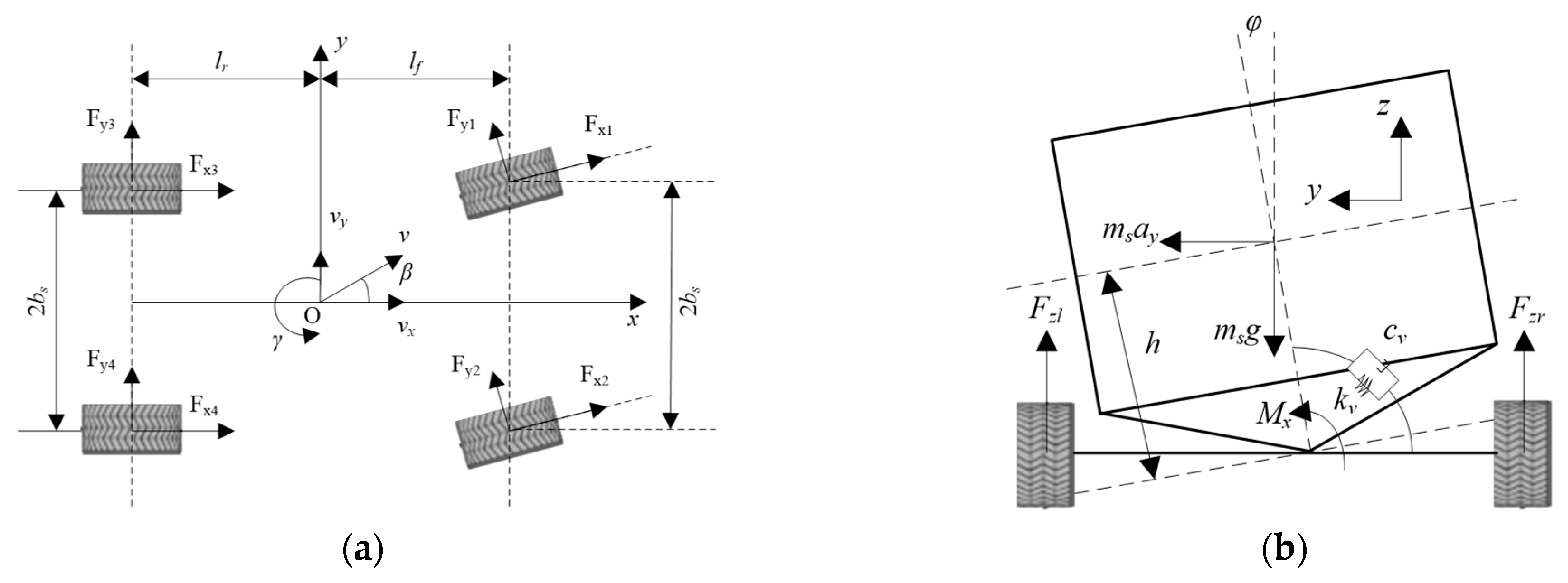
Building a mathematical model that can truly reflect the dynamic behavior of vehicles is the core prerequisite for the design of vehicle controllers and the implementation of motion-control algorithms. To this end, we set up a virtual three-dimensional reference coordinate system: its x-axis coincides with the longitudinal direction of the vehicle’s motion, the y-axis is perpendicular to the x-axis and points laterally, the z-axis is defined as the vertical direction, and the reference point is fixed to the vehicle’s center of mass. In the modeling process, the influence of air resistance and differences in tire mechanical properties is ignored. Figure 1 shows a schematic diagram of the dynamic model, including two perspectives [33]: the lateral dynamic model and the vertical dynamic model of the vehicle. Among them, the dynamic equation of the vehicle monorail model that integrates lateral and yaw degrees of freedom [12] can be expressed as

$$m\left({\dot{v}}_y+v_x\gamma \right)=F_{yf}+F_{yr},$$

(1)

$$I_z\dot{\gamma }=l_f{F}_{yf}-l_r{F}_{yr}+M_z,$$

(2)

where m is the overall vehicle mass, v_x is the longitudinal vehicle speed, v_y is the lateral vehicle speed, γ is the vehicle yaw rate, I_z is the vehicle’s moment of inertia around the z-axis, l_f and l_r are the distances from the vehicle’s center of mass to the front and rear axles, F_yf and F_yr are the lateral tire forces on the front and rear wheels, respectively, and M_z is the additional yaw moment and can be denoted as $M_z={\displaystyle \sum _{i=1}^4{F}_{xi}}\left[{\left(-1\right)}^i{b}_s\cos {\delta }_f+l_f\sin {\delta }_f\right]$, ${\delta }_f$ is the front-wheel steering angle, b_s is the half distance of front and rear wheels; and F_xi (i = 1, 2, 3, 4) is the tire force acting on the ith wheel. The vehicle model equation considering the dynamics of vehicle roll degrees of freedom can be expressed as

$$I_x\ddot{\varphi }=m_s{a}_{y}g+m_{s}gh-c_v\dot{\varphi }-k_v\varphi +M_x,$$

(3)

where $I_x$ is the moment of inertia of the entire vehicle around the x-axis, $\varphi$, $\dot{\varphi }$, and $\ddot{\varphi }$ are the vehicle roll angle, vehicle roll-angle velocity, and vehicle roll-angle acceleration, respectively. $m_s$ is the sprung mass, $a_y$ is the lateral acceleration of the vehicle, $g$ is the acceleration due to gravity, $h$ is the height of the vehicle’s center of mass from the horizontal ground, $k_v$ is the equivalent roll damping, $c_v$ is the equivalent roll stiffness, and $M_x$ is the roll moment.

Assuming that the front-wheel rotation angle of the vehicle is small and the tires are in a linear working area, the lateral tire force of the front and rear wheels can be expressed as

$$\begin{array}{l}{F}_{yf}=2C_f{\alpha }_f\\ F_{yr}=2C_r{\alpha }_r\end{array},$$

(4)

where C_f and C_r are the lateral stiffness of the front and rear tires, respectively, and α_f and α_r are the tire lateral angles of the front and rear tires, respectively. And the tire sideslip angle can be expressed as

$$\begin{array}{c}{\alpha }_f={\delta }_f-{\displaystyle \frac{l_f\gamma +v_y}{v_x}}\\ {\alpha }_r={\displaystyle \frac{l_r\gamma -v_y}{v_x}}\end{array},$$

(5)

where δ_f is the front-wheel steering angle. By combining the above equations, the vehicle dynamics model including lateral and roll dynamics can be derived as

$$\dot{\gamma }={\displaystyle \frac{C_r{l}_r-C_f{l}_f}{I_z}}\beta -{\displaystyle \frac{C_f{l}_f^2+C_r{l}_r^2}{I_z{v}_x}}\gamma +{\displaystyle \frac{C_f{l}_f}{I_z}}{\delta }_f+{\displaystyle \frac{1}{I_z}}{M}_z,$$

(6)

$$\dot{\beta }=-{\displaystyle \frac{C_f+C_r}{m{v}_x}}\beta -\left(1+{\displaystyle \frac{C_f{l}_f-C_r{l}_r}{m{v}_x^2}}\right)\gamma +{\displaystyle \frac{C_f}{m{v}_x}}{\delta }_f,$$

(7)

$$\ddot{\varphi }=-{\displaystyle \frac{h\left(C_f+C_r\right)m_s}{I_{x}m}}\beta +{\displaystyle \frac{h\left(-C_f{l}_f+C_r{l}_r\right)m_s}{I_x{v}_{x}m}}\gamma -{\displaystyle \frac{c_v}{I_x}}\dot{\varphi }+{\displaystyle \frac{m_{s}gh-k_v}{I_x}}\varphi +{\displaystyle \frac{h{C}_f{m}_s}{I_{x}m}}{\delta }_f+{\displaystyle \frac{1}{I_x}}{M}_x,$$

(8)

where $\beta$ is the vehicle sideslip angle, and it can be denoted as $\beta =\arctan \left(v_y/v_x\right)\approx v_y/v_x$.

2.2. Trajectory-Tracking Model

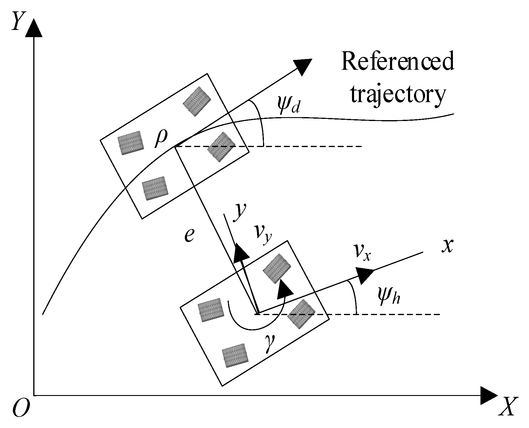
In order to comprehensively characterize the kinematic performance of unmanned vehicles in the trajectory-tracking stage at the mathematical level, this paper constructs a trajectory-tracking kinematic model and provides its structural schematic in Figure 2. In this diagram, the global geodetic coordinate system XOY is first constructed with the ground as the reference; subsequently, two core state variables, lateral position error and heading angle error, were introduced to quantitatively evaluate the degree of deviation of the unmanned vehicle from the expected path. The specific expression for heading angle error is as follows

$$\psi ={\psi }_h-{\psi }_d,$$

(9)

where ψ is the heading error, ψ_h is the real heading angle of vehicle, and ψ_d is the referenced heading angle of vehicle. By taking the derivative of Equation (9), we can obtain

$$\dot{\psi }=\gamma -\rho v_x,$$

(10)

where ρ is the curvature of referenced trajectory. The lateral deviation of trajectory tracking is the lateral offset between the center of mass of the unmanned vehicle and the reference trajectory, and its differential equation can be expressed as

$$\dot{e}=v_x\sin \psi +v_y\cos \psi ,$$

(11)

where e represents the lateral offset. Assuming a small heading deviation, then Equation (11) can be expressed as

$$\dot{e}=v_x\psi +v_y,$$

(12)

Then, by combining Equations (7) and (8) with Equations (10) and (12), the trajectory tracking control model of intelligent vehicle can be obtained as

$$\begin{array}{l}{\dot{x}}_1=x_2\\ {\dot{x}}_2=-{\displaystyle \frac{C_f+C_r}{m{v}_x}}{x}_2+{\displaystyle \frac{C_f+C_r}{m}}{x}_3+{\displaystyle \frac{C_r{l}_r-C_f{l}_f}{m{v}_x}}{x}_4+{\displaystyle \frac{C_f}{m}}u+{\displaystyle \frac{C_r{l}_r-C_f{l}_f}{m\rho }}-{\displaystyle \frac{v_x^2}{\rho }}\\ {\dot{x}}_3=x_4\\ {\dot{x}}_4={\displaystyle \frac{C_r{l}_r-C_f{l}_f}{I_z{v}_x}}{x}_2+{\displaystyle \frac{C_f{l}_f-C_r{l}_r}{I_z}}{x}_3-{\displaystyle \frac{C_f{l}_f^2+C_r{l}_r^2}{I_z{v}_x}}{x}_4+{\displaystyle \frac{2C_f{l}_f}{I_z}}u-{\displaystyle \frac{C_f{l}_f^2+C_r{l}_r^2}{I_z\rho }}\end{array},$$

(13)

where the system state variables can be written as $x_1=e$, $x_2=\dot{e}$, $x_3=\psi$, $x_4=\dot{\psi }$, and the input is written as $U={\delta }_f$.

3. Coordinated Control of Trajectory Tracking and Vehicle Stability Based on State Estimation

3.1. Hierarchical Control Strategy

The vehicle control strategy consists of three parallel and continuously interactive functional modules: trajectory tracking, state estimation, and lateral-roll integrated control, which exchange information in real time through a shared data bus. In the vehicle trajectory-tracking controller, the controller compares the lateral deviation and heading error between the actual vehicle position and the expected trajectory based on the reference trajectory information. The trajectory-tracking controller adopts high-order sliding mode control to achieve the required front-wheel steering angle control based on the latest lateral deviation and heading deviation and their change rates. The state-estimation module utilizes an extended Kalman filter to process the measurement signals of front-wheel steering angle, vehicle speed, yaw rate, yaw moment, and roll moment as the known inputs, and uses a discretized vehicle dynamics model for dynamic prediction and correction, thereby estimating key state variables such as vehicle sideslip angle, roll angle, and roll rate, and inputting the results to the corresponding control module. The integrated control module for lateral-roll stability is implemented based on double power approach law sliding mode control. The stability controller receives the front-wheel steering angle control quantity from the trajectory tracking control module, and combines it with the state estimation quantities of the vehicle sideslip angle, yaw rate, roll angle, and roll-angle velocity provided by the state estimation module. Applying a double-power sliding mode convergence law, it quickly calculates the actual yaw moment and roll moment that need to be applied to the vehicle chassis at each moment, and directly drives the actuator action. The collaborative control strategy, which integrates trajectory tracking and stability control based on state estimation, is illustrated in Figure 3.

3.2. Vehicle Trajectory-Tracking Control Method

In order to clearly express the design process of the trajectory-tracking controller, it is defined that $a_{t1}=-{\displaystyle \frac{C_f+C_r}{m{v}_x}}$, $a_{t2}={\displaystyle \frac{C_f+C_r}{m}}$, $a_{t3}={\displaystyle \frac{C_r{l}_r-C_f{l}_f}{m{v}_x}}$, $a_{t4}={\displaystyle \frac{C_r{l}_r-C_f{l}_f}{I_z{v}_x}}$, $a_{t5}={\displaystyle \frac{C_f{l}_f-C_r{l}_r}{I_z}}$, $a_{t6}=-{\displaystyle \frac{C_f{l}_f^2+C_r{l}_r^2}{I_z{v}_x}}$, $b_{t1}={\displaystyle \frac{C_f}{m}}$, $b_{t2}={\displaystyle \frac{2C_f{l}_f}{I_z}}$, $d_{t1}={\displaystyle \frac{C_r{l}_r-C_f{l}_f}{m\rho }}-{\displaystyle \frac{v_x^2}{\rho }}$, $d_{t2}=-{\displaystyle \frac{C_f{l}_f^2+C_r{l}_r^2}{I_z\rho }}$. Then, the trajectory-tracking model in Equation (13) be expressed as

$$\begin{array}{l}{\dot{x}}_1=x_2\\ {\dot{x}}_2=f_1\left(x\right)+b_{1}U\\ {\dot{x}}_3=x_4\\ {\dot{x}}_4=f_2\left(x\right)+b_{2}U\end{array},$$

(14)

where the state variable x is defined as $x={[x_1 x_2 x_3 x_4]}^T$, $d_{t1}$ and $d_{t2}$ are known interferences of the system, and there is $f_1\left(x\right)=a_{t1}{x}_2+a_{t2}{x}_3+a_{t3}{x}_4+d_{t1}$, $f_2\left(x\right)=a_{t4}{x}_2+a_{t5}{x}_3+a_{t6}{x}_4+d_{t2}$. The vehicle trajectory-tracking control requires real-time vehicle dynamics control to minimize the lateral and heading deviations between the actual vehicle trajectory and the reference trajectory. For system (12), it is necessary to design a trajectory-tracking controller to ensure the system state approaches zero.

In the design process of the sliding-mode controller, the inherent flutter problem cannot be ignored. The negative mechanism of chatter in a vehicle controller during trajectory tracking and lateral-roll cooperative control can be traced back to the coupling effect of high-frequency switching law inherent in sliding mode control, vehicle dynamics and actuator physical characteristics. The traditional first-order sliding mode directly applies the symbol function to the control channel, and its ideal switching frequency tends to be infinite. However, the bandwidth of the vehicle chassis execution layer is limited, which means that the nominal ideal sliding-mode surface cannot be accurately maintained. At this time, the system state crosses back and forth at a finite frequency near the sliding-mode surface, resulting in a limit-cycle oscillation, the amplitude and frequency of which are affected by the interaction of tire stiffness, actuator hysteresis, and chassis lateral and vertical dynamics. This oscillation not only amplifies the lateral deviation and heading deviation, but also induces the pitch roll resonance of the sprung mass through the coupling path of lateral acceleration and roll torque, so that the vertical load is redistributed, further weakening the linear controllable range of tire cornering force, and finally forming a “flutter instability” positive feedback.

The vehicle trajectory-tracking model in Equation (14) is a typical underactuated system. To address this issue, and to weaken the side effects caused by the above mechanism, the sliding surface s can be defined as

$$s=c_1{x}_1+c_2{x}_2+c_3{x}_3+c_4{x}_4,$$

(15)

where c₁, c₂, c₃, and c₄ are normal numbers. By taking the first derivative of the sliding surface, the following equation can be obtained

$$\begin{array}{l}\dot{s}=c_1{\dot{x}}_1+c_2{\dot{x}}_2+c_3{\dot{x}}_3+c_4{\dot{x}}_4=c_1{x}_2+c_2{f}_1+c_2{b}_{1}U+c_3{x}_4+c_4{f}_2+c_4{b}_{2}U\\ =\left[c_1{x}_2+c_2{f}_1+c_3{x}_4+c_4{f}_2\right]+\left(c_2{b}_1+c_4{b}_2\right)U=F(x)+G(x)U\end{array},$$

(16)

where $F(x)=c_1{x}_2+c_2{f}_1+c_3{x}_4+c_4{f}_2$, $G(x)=c_2{b}_1+c_4{b}_2$. Obviously, $F(x)$ is continuous and first-order differentiable, while $G(x)$ is a constant. It can be seen that the first derivative of s with respect to time has a control variable, namely the control input U.

By taking the first derivative of Equation (16) again, we can obtain

$$\ddot{s}=\dot{F}(x)+G(x)\dot{U},$$

(17)

Equation (17) can be written in the form of an integral chain as follows

$$\left\{\begin{array}{l}{\dot{s}}_1=s_2\hfill \\ {\dot{s}}_2=\dot{F}(x)+G(x)\dot{U}\hfill \end{array}\right.,$$

(18)

$\dot{U}$ is defined as the virtual control quantity, where $s_1=s$, $s_2=\dot{s}$. To avoid problems such as signal noise caused by multiple derivative calculations, in Equation (18), an arbitrary-order sliding-mode robust differentiator is used for high-precision approximation of $\dot{F}(x)$. The approximation result is represented by $\dot{\overline{F}}(x)$, and ${\Delta }_F(x)=\dot{F}(x)-\dot{\overline{F}}(x)$ is the approximation error. In finite time, ${\Delta }_F(x)$ approaches 0; If $G(x)$ is split into two items, then there is $G(x)=\overline{G}(x)+{\Delta }_G(x)$. Thus, the system (18) can be written in the following form with uncertain terms

$$\left\{\begin{array}{l}{\dot{s}}_1=s_2\hfill \\ {\dot{s}}_2=\dot{\overline{F}}(x)+{\Delta }_F(x)+(\overline{G}(x)+{\Delta }_G(x))\dot{U}\hfill \end{array}\right.,$$

(19)

where $\dot{\overline{F}}(x)$ and $\overline{G}(x)$ are the nominal parts of $\dot{F}(x)$ and $G(x)$ in the controller design process, respectively. The uncertain part of $\dot{F}(x)$ is represented by a bounded function ${\Delta }_F(x)$, and there exists a known nonlinear function $\rho (x)$ and a known constant $1⩾\delta >0$ that satisfy the following conditions

$$\left\{\begin{array}{l}‖{\Delta }_F\left(x\right)\hspace{0.17em}-{\Delta }_G\left(x\right)\hspace{0.17em}{\overline{G}}^{-1}\left(x\right)\hspace{0.17em}\dot{\overline{F}}\left(x\right)\hspace{0.17em}‖⩽\rho \left(x\right)\hfill \\ ‖{\Delta }_G\left(x\right)\hspace{0.17em}{\overline{G}}^{-1}\left(x\right)\hspace{0.17em}‖⩽1\hspace{0.17em}-\delta \hfill \end{array}\right.,$$

(20)

where $‖\cdot ‖$ is defined as the 2-norm.

Next, it is necessary to design and analyze the stability of a high-order sliding-mode controller for vehicle trajectory tracking. By defining the sliding surface s, the input-output relationship between the sliding surface and the virtual control variable $\dot{U}$ can be effectively established. The integral chain form of the following single-input–single-output is represented as

$$\left\{\begin{array}{l}{\dot{s}}_1=s_2\hfill \\ {\dot{s}}_2=w_{\mathrm{nom} }\hfill \end{array}\right.,$$

(21)

Therefore, the feedback control law in the equation can be expressed as $w_{\mathrm{nom} }(s)=-k_1\mathrm{sgn}\left(s_1\right){\left|s_1\right|}^{{\displaystyle \frac{1}{2}}}-k_2\mathrm{sgn}\left(s_2\right){\left|s_2\right|}^{{\displaystyle \frac{2}{3}}}$, and the normal numbers $k_1$ and $k_2$ can be used to ensure that $p^2+k_{2}p+k_1$ is Hurwitz. It can be considered that system (21) can converge to the origin in finite time. Then, design the auxiliary control input in the following form

$$\left\{\begin{array}{l}w(s)=w_{\mathrm{nom} }(s)+w_{\mathrm{disc} }(s,{\sigma }_{\mathrm{aux}})\hfill \\ {\dot{\sigma }}_{\mathrm{aux} }=-w_{\mathrm{nom} }(s)\hfill \end{array}\right.\hspace{0.33em}\hspace{0.33em},$$

(22)

where $s={[s_1,s_2]}^{\mathrm{T}}$. The sliding surface related to $w_{\mathrm{disc}}(s)$ is defined as $\sigma =s_2+{\sigma }_{\mathrm{aux}}$ and $w_{\mathrm{disc}}=-\eta \mathrm{sgn}(\sigma )$. Then, the control gain $\eta$ can be expressed as

$$\eta ⩾{\displaystyle \frac{(1-\delta )\left|w_{\mathrm{nom}}\right|+\rho +\epsilon }{\delta }},$$

(23)

where $\epsilon$ is a small normal number.

In the system (17), assuming that Equation (20) holds, its high-order sliding mode control law can be expressed as

$$\dot{U}={\overline{G}}^{-1}(-\dot{\overline{F}}+w_{\mathrm{nom}}(s)+w_{\mathrm{disc}}(s,{\sigma }_{\mathrm{aux}})),$$

(24)

Thus, the system can converge to zero in finite time. Under the control law (24), the closed-loop equation of system (17) can be expressed as

$$\left\{\begin{array}{l}{\dot{s}}_1=s_2\hfill \\ {\dot{s}}_2=(1+{\Delta }_G{\overline{G}}^{-1})(w_{\mathrm{nom}}(s)+w_{\mathrm{disc}}(s,{\sigma }_{\mathrm{aux}}))-{\Delta }_G{\overline{G}}^{-1}\dot{\overline{F}}+{\Delta }_F\hfill \end{array}\right.,$$

(25)

By selecting the following form of Lyapunov function $V=0.5{\sigma }^2$, according to Equations (22)–(25), it can be obtained as

$$\begin{array}{l}\dot{V}=\sigma ({\dot{s}}_2+{\dot{\sigma }}_{\mathrm{aux}})=\sigma ((1+{\Delta }_G{\overline{G}}^{-1})w_{\mathrm{disc}}-{\Delta }_G{\overline{G}}^{-1}\dot{\overline{F}}+{\Delta }_F+{\Delta }_G{\overline{G}}^{-1}{w}_{\mathrm{nom}})\\ =\sigma (-\eta (1+{\Delta }_G{\overline{G}}^{-1})\mathrm{sgn}(\sigma )-{\Delta }_G{\overline{G}}^{-1}\dot{\overline{F}}+{\Delta }_F+{\Delta }_G{\overline{G}}^{-1}{w}_{\mathrm{nom}})\\ ⩽-\eta \left|\sigma \right|+(1-\delta )\eta \left|\sigma \right|+(1-\delta )\left|w_{\mathrm{nom}}\right|\left|\sigma \right|+\rho \left|\sigma \right|\\ ⩽(-\delta \eta +(1-\delta )|w_{\mathrm{nom}}|+\rho )\left|\sigma \right|⩽-\epsilon \left|\sigma \right|⩽-\epsilon \sqrt{2}\sqrt{V}\le 0\end{array},$$

(26)

Therefore, under uncertain conditions, the trajectory of system (17) reaches the sliding mode set $\{s\in X:\sigma =0\}$ after a finite time $T_f⩾{\displaystyle \frac{V(0)}{\sqrt{2\epsilon }}}$.

According to assumption (20), $(1+{\Delta }_c{\tilde{G}}^{-1})$ is reversible. According to Equations (10) and (18), when $\dot{\sigma }=0$, $w_{disc}$ satisfies the following condition

$$w_{disc}={(1+{\Delta }_G{\overline{G}}^{-1})}^{-1}({\Delta }_G{\overline{G}}^{-1}\dot{\overline{F}}-{\Delta }_F-{\Delta }_G{\overline{G}}^{-1}{w}_{nom}),$$

(27)

Therefore, when $t>T_f$, the closed-loop motion equation of the system is expressed as

$$\left\{\begin{array}{l}{\dot{s}}_1=s_2\hfill \\ {\dot{s}}_2={\Delta }_G{\overline{G}}^{-1}{w}_{nom}\hfill \end{array}\right.,$$

(28)

According to Equation (21), the control law $w_{nom}$ can ensure that the system (28) converges in finite time. Therefore, the second-order sliding-mode motion of $s={[s_1,s_2]}^T$ is established such that $s_1=s_2=0$. Given the initial control variable $U(0)$, by integrating Equation (24), the actual feedback control law of vehicle front-wheel steering angle can be obtained as

$$U=U(0)+{\displaystyle \int {\overline{G}}^{-1}}(-\dot{\overline{F}}+w_{nom}(s)+w_{disc}(s,{\sigma }_{aux}))\mathrm{d}\tau ,$$

(29)

From this, it can be seen that the introduction of the integral term in Equation (29) directly includes the switching term in the first derivative of the actual control variable, and the actual control variable does not contain high-frequency switching, thus achieving the goal of eliminating control chattering.

3.3. Vehicle Lateral-Roll Integrated Control Method Based on State Estimation

The vehicle dynamics models in Equations (6)–(8) can be transformed into discrete-state space equations in the following form

$$\begin{array}{l}{x}_{k+1}=A_k{x}_k+B_k{u}_k+w_k\\ y_k=C_k{x}_k+v_k\end{array},$$

(30)

where x_k+1 is the system-state quantity of the discrete model; y_k+1 is the system measurement quantity of the discrete model; A_k+1, B_k+1, C_k+1 represent the state-transition matrix, input matrix, and measurement matrix of the discrete model, respectively; and w_k and v_k are the process noise and measurement noise, respectively. w_k and v_k are both Gaussian white noise vectors and are uncorrelated with each other. The covariance matrices of process noise and measurement noise can be written as Q_k and R_k, respectively. Kalman filtering is a widely used and effective estimation algorithm, which has been proven to have good state estimation performance in many studies. Extended Kalman filter can linearize the nonlinearity of the system, which has superior performance for state estimation of complex systems and is more suitable for real vehicle applications. According to the state-space equation in Equation (30), the iterative steps of the extended Kalman filter can be expressed as

(1)

Time propagation of status information.

The initialization status is

$$x_{0/0}=E\left(x_0\right),P_{0/0}=E\left[\left(x-x_0\right){\left(x-x_0\right)}^T\right],$$

(31)

where x₀ is the initial state vector, and P₀ is the error covariance matrix. The predicted system state at a fixed step size can be expressed as

$${\widehat{x}}_{k+1/k}=A_k{\widehat{x}}_k+B_k{u}_k,$$

(32)

The variance of prediction error at the current step size can be expressed as

$$P_{k+1/k}={\Phi }_k{P}_{k/k}{\Phi }_k^T+Q_k,$$

(33)

where P_k is the covariance matrix of the system-state estimation error, ${\Phi }_k=I+A_{k}T$, and T is the filtering period of the Kalman filter.

(2)

Status information measurement update.

Based on the previous prediction variance, the feedback gain matrix of the further calculated state estimation can be expressed as

$$K_{k+1}=P_{k+1/k}{C}_{k+1}^T{\left(C_{k+1}{P}_{k+1/k}{C}_{k+1}^T+R_{k+1}\right)}^{-1},$$

(34)

where K_k+1 is the state feedback matrix. Then, based on the feedback gain matrix, the estimated value of the state filter at the current time can be expressed as

$${\widehat{x}}_{k+1/k+1}={\widehat{x}}_{k+1/k}+K_{k+1}\left[y_{k+1}-C_{k+1}{x}_{k+1/k}\right].$$

(35)

Finally, the variance of the filtering estimation error at the next moment is calculated again to enter the next iteration of estimation, which is

$$P_{k+1/k+1}=\left(I-K_{k+1}{C}_{k+1}\right)P_{k+1/k}.$$

(36)

By using the extended Kalman filter mentioned above, a method for estimating the driving state of the entire vehicle can be designed in conjunction with the vehicle dynamics model. The system-state variable is $x_k={\left[\begin{array}{cccc}{\gamma }_k& {\beta }_k& {\varphi }_k& {\dot{\varphi }}_{v,k}\end{array}\right]}^T$, the input variable is $u_k={\left[\begin{array}{cc}{\delta }_k& {\gamma }_k\end{array}\right]}^T$, and the measurement variable is $y_k=a_{y,k}$. Here, a_x and a_y are the longitudinal acceleration and lateral acceleration of the vehicle, respectively, and satisfy the following formula

$$\begin{array}{l}{a}_x={\dot{v}}_x-\gamma v_y\\ a_y={\dot{v}}_y+\gamma v_x\end{array}.$$

(37)

According to Equation (37), the formula for lateral acceleration can be derived as

$$a_y=-{\displaystyle \frac{C_f{l}_f-C_r{l}_r}{m{v}_x}}\gamma -{\displaystyle \frac{C_f+C_r}{m}}\beta +{\displaystyle \frac{C_f}{m}}\delta .$$

(38)

By discretizing the equation, the required measurement equation for the extended Kalman filter can be obtained.

According to the above vehicle-state Kalman filtering estimation method, the estimated values of the vehicle’s center of mass roll angle and roll angle can be obtained. Then, treat this value as a soft sensing value measured by a virtual sensor and use it as an input for the vehicle’s lateral-roll integrated controller. To simplify representation and facilitate controller design, it is defined as $a_{s1}={\displaystyle \frac{C_r{l}_r-C_f{l}_f}{I_z}}$, $a_{s2}=-{\displaystyle \frac{C_f{l}_f^2+C_r{l}_r^2}{I_z{v}_x}}$, $a_{s3}=-{\displaystyle \frac{C_f+C_r}{m{v}_x}}$, $a_{s4}=-\left(1+{\displaystyle \frac{C_f{l}_f-C_r{l}_r}{m{v}_x^2}}\right)$, $a_{s5}=-{\displaystyle \frac{h\left(C_f+C_r\right)m_s}{I_{x}m}}$, $a_{s6}={\displaystyle \frac{h\left(-C_f{l}_f+C_r{l}_r\right)m_s}{I_x{v}_{x}m}}$, $a_{s7}=-{\displaystyle \frac{c_v}{I_x}}$, $a_{s8}={\displaystyle \frac{m_{s}gh-k_v}{I_x}}$, $b_{s1}={\displaystyle \frac{C_f{l}_f}{I_z}}{\delta }_f$, $b_{s2}={\displaystyle \frac{1}{I_z}}$, $b_{s3}={\displaystyle \frac{C_f}{m{v}_x}}{\delta }_f$, $b_{s4}={\displaystyle \frac{h{C}_f{m}_s}{I_{x}m}}{\delta }_f$, $b_{s5}={\displaystyle \frac{1}{I_x}}$. In order to achieve integrated controller design, Equations (6)–(8) are represented as the following state-space equations

$${\dot{x}}_s=f_s\left(x\right)+g_s\left(x\right)u+\epsilon .$$

(39)

where $x_s={\left[\begin{array}{cccc}{x}_{s1}& x_{s2}& x_{s3}& x_{s4}\end{array}\right]}^T={\left[\begin{array}{cccc}\gamma & \beta & {\varphi }_v& {\dot{\varphi }}_v\end{array}\right]}^T$, $u={\left[\begin{array}{cc}{u}_{s1}& u_{s2}\end{array}\right]}^T={\left[\begin{array}{cc}{M}_z& M_x\end{array}\right]}^T$, $f_s\left(x\right)=\left[\begin{array}{c}{a}_{s1}{x}_{s2}+a_{s2}{x}_{s1}+b_{s1}\\ a_{s3}{x}_{s2}+a_{s4}{x}_{s1}+b_{s3}\\ x_{s4}\\ a_{s5}{x}_{s2}+a_{s6}{x}_{s1}+a_{s7}{x}_{s4}+a_{s8}{x}_{s3}+b_{s5}\end{array}\right]$, $g\left(x\right)=\left[\begin{array}{cc}{b}_{s2}& 0\\ 0& 0\\ 0& 0\\ 0& b_{s5}\end{array}\right]$, $\epsilon$ is the amount of system interference.

For the vehicle system (39), in order to improve the control accuracy and anti-interference ability of the vehicle controller, the sliding-surface convergence law is designed as a double-power convergence law in the following form

$$\dot{s}=-k_1{\left|s\right|}^{m_1}\mathrm{sgn}\left(s\right)-k_2{\left|s\right|}^{m_2}\mathrm{sgn}\left(s\right).$$

(40)

where $k_1>0$, $k_2>0$, $m_1>1$, $0<m_2<1$. According to the sliding-mode convergence law mentioned above, when the system state deviates from the sliding mode, the sliding-mode approaching speed accelerates and the system can quickly approach the sliding surface. When the system state approaches the sliding surface, in order to avoid excessive chattering, this sliding-mode convergence law can reduce the adjustment amplitude of the sliding mode. If the reference state of the vehicle controller is $x_d$, then the tracking error is $e=x-x_d$, and the sliding surface can be defined as

$$s=k_{s}e+\dot{e}.$$

(41)

where $k_s$ is the sliding-mode-control parameter greater than 0. Therefore, it can be concluded that the sliding-mode-control rate under this convergence law is

$$u={\displaystyle \frac{1}{g\left(x\right)}}({\displaystyle \frac{1}{k_s}}\left(-k_1{\left|s\right|}^{m_1}\mathrm{sgn}\left(s\right)-k_2{\left|s\right|}^{m_2}\mathrm{sgn}\left(s\right)\right.\left.+k_s{\dot{x}}_d-\ddot{e}\right)\left.-f\left(x\right)-\epsilon \right).$$

(42)

To demonstrate the convergence of the sliding-mode controller, the Lyapunov function is selected as $V={\displaystyle \frac{1}{2}}{s}^2$. By taking the derivative of the Lyapunov function, we can obtain

$$\dot{V}=s\dot{s}=s\mathrm{sgn}\left(s\right)\left(-k_1{\left|s\right|}^{m_1}-k_2{\left|s\right|}^{m_2}\right).$$

(43)

It can be observed that $\dot{V}\le 0$ is constant, indicating that the designed sliding-mode controller tends to be stable.

4. Result Verification

In order to verify the application effect of the state-estimation-based vehicle trajectory tracking and stability collaborative control strategy designed in the article, simulation verification and analysis were conducted based on a joint simulation model of CarSim V8.02 and Simulink R2022b. Among them, the CarSim software was used to provide a dynamic model of the entire vehicle, and the vehicle-state estimation module and vehicle-coupling control module were built in Simulink software. Corresponding simulation conditions were selected for joint simulation experiments. The vehicle parameters in the simulation are shown in

Table 1. Vehicle parameters.

Vehicle Parameters	Numerical Values and Units
Vehicle mass	860 kg
Distance from center of mass to front/rear axle	1.2 m
Half wheelbase	0.7 m
Effective radius of wheels	0.3 m
Front/rear wheel lateral stiffness	50,000 N/rad
Sprung mass	560 kg
Equivalent lateral stiffness	50,000 N/rad
Equivalent roll damping	5000 N·s/(m·rad)
Height of vehicle mass center	0.65 m
Moment of inertia	1000 kg·m2

. In addition, the simulation test conditions are selected for lane-changing scenarios with a vehicle speed of 20 m/s and a road adhesion coefficient of 1.0.

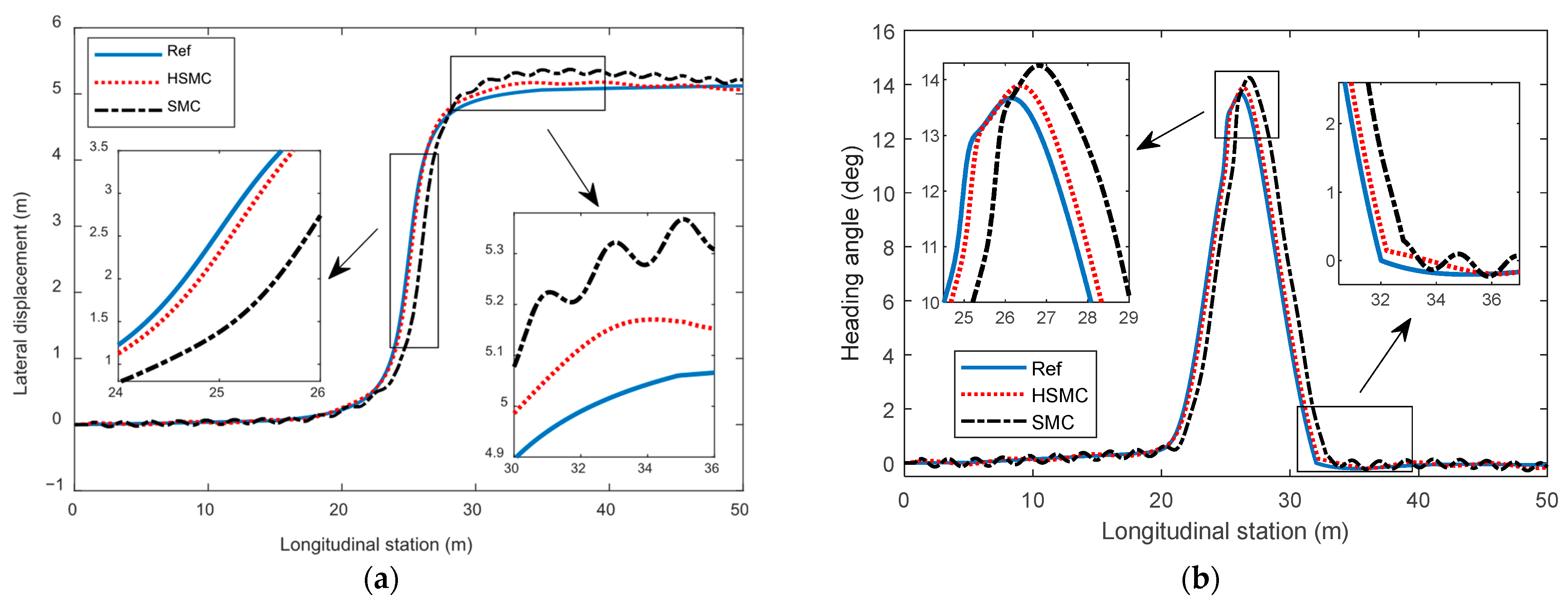
In order to reflect the vehicle application effect of the proposed sliding-mode-control algorithm, a common conventional sliding-mode-control algorithm based on switching control law is selected as the comparison benchmark. Under driving conditions involving lane-changing trajectory-tracking control, the obtained vehicle trajectory-tracking control results are shown in Figure 4. According to the actual vehicle travel trajectory results under different control methods, it can be seen that the vehicle travel trajectory obtained under the HSMC algorithm is significantly closer to the reference trajectory overall. While the conventional sliding-mode-control algorithm can track the general trend of the reference trajectory, it suffers from notable lag and deviation, particularly during rapid lane-changing maneuvers. Through the local magnification of the trajectory curve, it can be observed that the vehicle trajectory under the HSMC algorithm has faster response capability and higher tracking accuracy during rapid lane changes. Compared to the sliding-mode-control algorithm, the overall vehicle trajectory curve has a very minor time-delay problem. At the same time, when the vehicle changes lanes and needs to return to straight driving, the trajectory curve obtained by the conventional SMC algorithm exhibits significant oscillations and fluctuations, which are caused by the inherent chattering problem of the sliding-mode-control algorithm and switching control law. In contrast, the proposed HSMC algorithm can make the vehicle’s driving trajectory smoother and converge faster.

The trend of changes in vehicle heading angle can better reflect the changes in the direction of vehicle travel. According to the comparison results of vehicle heading angles in Figure 4, it can also be observed that there is a certain degree of lag in the tracking reference value of the vehicle heading angle under sliding-mode control, which is the direct reason for the lag of the vehicle driving trajectory curve compared to the reference trajectory curve under this algorithm. In contrast, the proposed high-order sliding-mode-control algorithm can ensure that the vehicle heading change can timely track the change requirements of the reference heading angle. Through local magnification, it can be seen that under the SMC algorithm, there is still a certain degree of fluctuation and oscillation in the amplitude of the vehicle heading angle after the vehicle trajectory returns to normal, which is also the direct reason for the oscillation of the vehicle’s driving trajectory at this time. The vehicle driving trajectory under the HSMC algorithm can track the trend of the reference heading angle in real time and accurately, and the overall tracking accuracy and dynamic response capability have been significantly improved.

The lateral deviation and heading deviation in the process of vehicle trajectory-tracking control can more intuitively reflect the trajectory-tracking accuracy under different control methods. Therefore, the error results of vehicle trajectory-tracking control were statistically analyzed, as shown in Figure 5. During the period when the vehicle is driving in a straight line and has not changed lanes, the lateral deviation of the vehicle under the two control methods is basically the same and fluctuates around zero values. When the vehicle changes lanes quickly, the lateral deviation of trajectory tracking under SMC algorithm increases sharply and the maximum amplitude is close to 1.5 m. In contrast, the lateral deviation of trajectory tracking under HSMC algorithm is well suppressed, with a maximum value of about 0.25 m, which is significantly reduced compared to SMC. At the same time, when the vehicle changes lanes and needs to continue driving in a straight line, the lateral deviation of the vehicle trajectory under the HSMC algorithm can quickly and smoothly converge and eventually approach zero. Under the SMC algorithm, there is a certain degree of overshoot in the lateral deviation of vehicle trajectories, which decreases to zero at the maximum amplitude and then increases in the opposite direction. Subsequently, its amplitude convergence speed is significantly slower and there is a significant oscillation phenomenon. This indicates that SMC algorithm is inferior to HSMC in terms of dynamic adjustment response capability and tracking accuracy.

The deviation in vehicle trajectory-tracking heading also shows the same trend of change. According to the comparison of heading deviation, it can be seen that during the period when the vehicle is traveling in a straight line and has not changed lanes, the heading angle of the vehicle under the two control algorithms remains basically unchanged around zero. When the vehicle needs to change lanes, the heading deviation of the vehicle under the HSMC algorithm is relatively small and its maximum deviation amplitude is about 1 deg, indicating that the heading of the vehicle under the HSMC algorithm is close to the reference trajectory requirement, thus ensuring good trajectory-tracking performance. In contrast, the vehicle trajectory heading deviation under the SMC algorithm increases rapidly in the initial stage of lane changing and reaches a deviation of nearly 3 deg. Then, during the process of the vehicle trajectory returning to normal, the heading deviation of the vehicle trajectory under the SMC algorithm increases in the opposite direction, which is also the direct reason for the occurrence of control overshoot in the lateral deviation of the vehicle trajectory. At the same time, the fluctuation and oscillation of vehicle heading deviation under SMC algorithm are more obvious, which leads to the oscillation of vehicle driving trajectory. Overall, the HSMC algorithm can significantly improve the vehicle trajectory-tracking control effect compared to SMC by providing fast heading tracking control and precise trajectory error-tracking suppression.

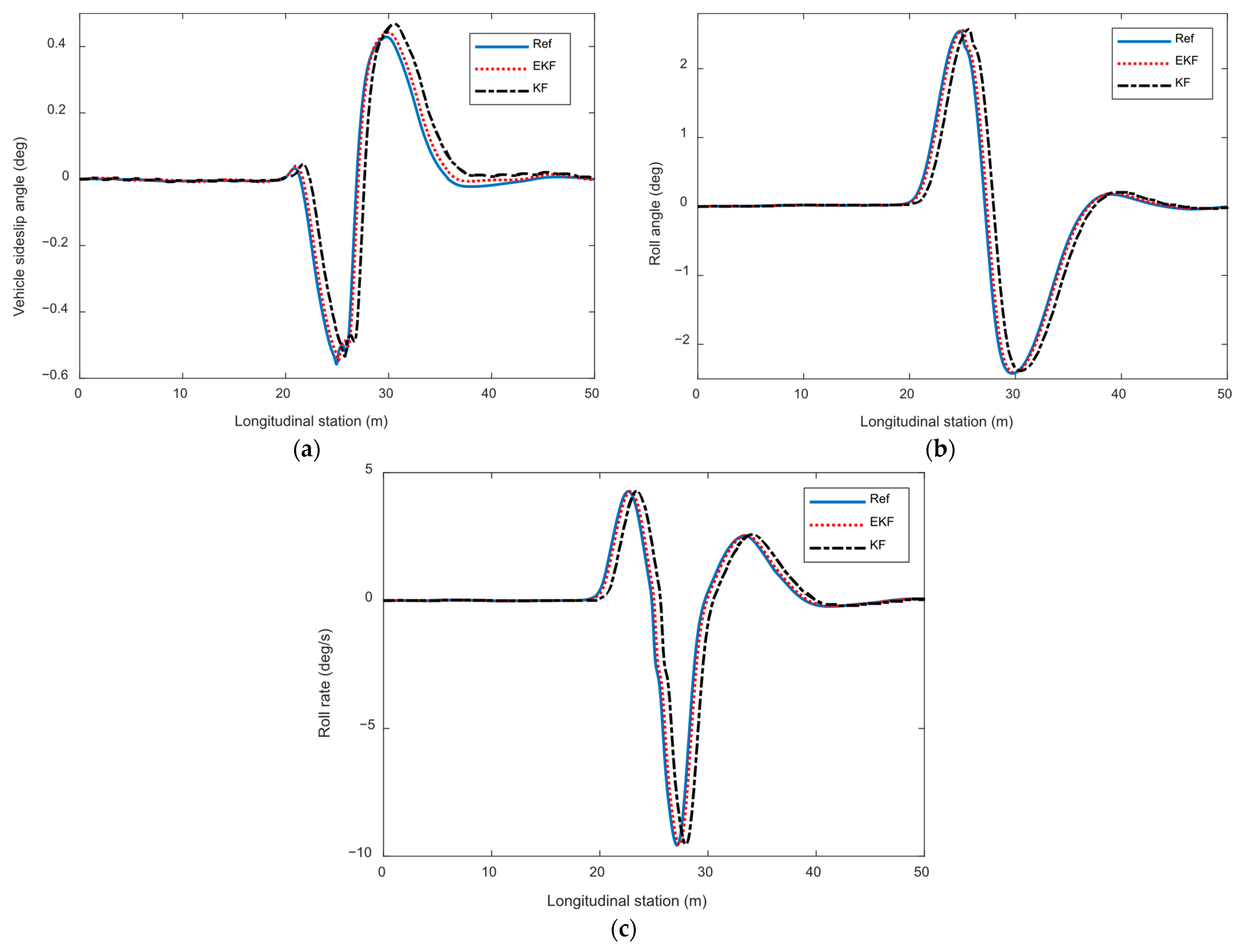
While analyzing the effectiveness of vehicle trajectory-tracking control, it is necessary to simultaneously consider the stability control effect of the vehicle. At this point, the performance of vehicle-state estimation based on EKF is one of the important factors affecting the effectiveness of vehicle stability control. The comparative results of vehicle-state estimation are shown in Figure 6. Overall, the Kalman filter algorithm can accurately calculate the vehicle’s center of mass roll angle, roll angle, and roll-angle velocity, and the estimated vehicle trajectory curve is in good agreement with the actual values. During the rapid lane-change process of vehicles, the vehicle state changes sharply, and there is a certain degree of time delay and amplitude deviation in the vehicle-state estimation results under the KF algorithm. On the other hand, EKF can relatively maintain good estimation performance, and the vehicle-state estimation results based on EKF algorithm have a certain degree of improvement in real-time performance, convergence speed, and overall estimation accuracy compared to KF. This indicates that the overall performance of the proposed estimation method can meet the requirements of vehicle control inputs.

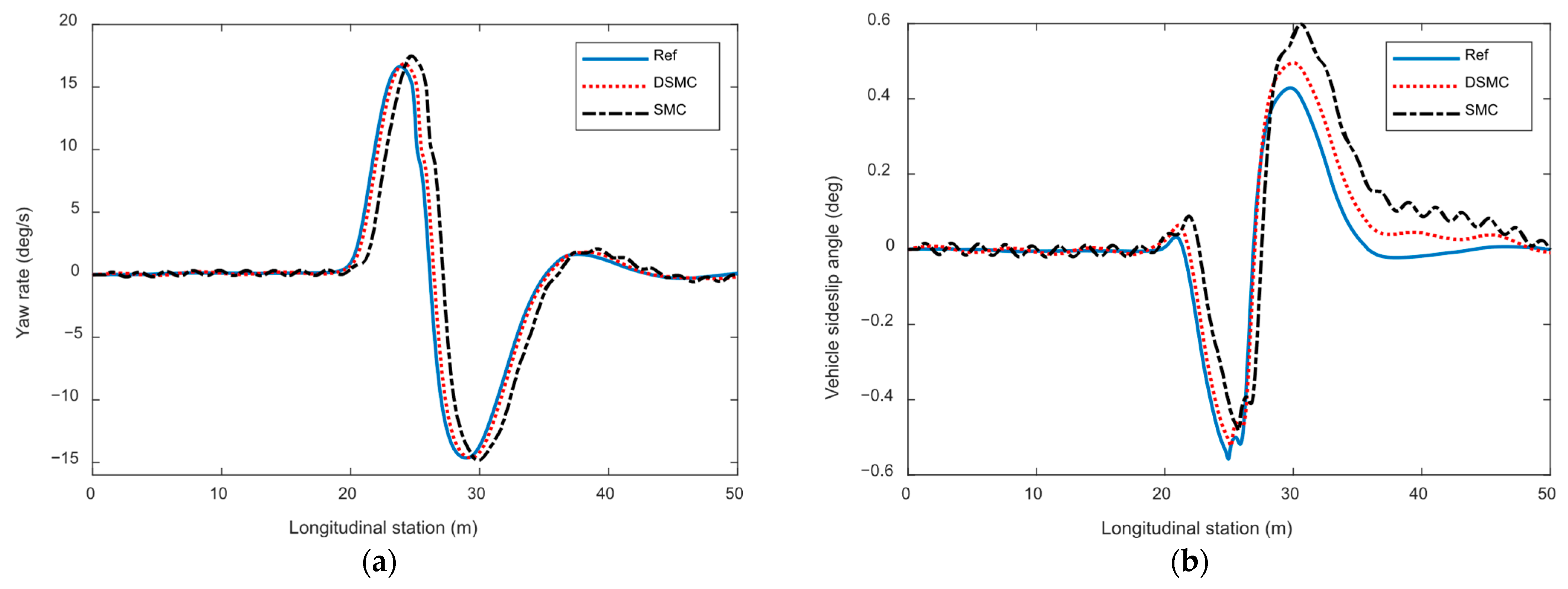
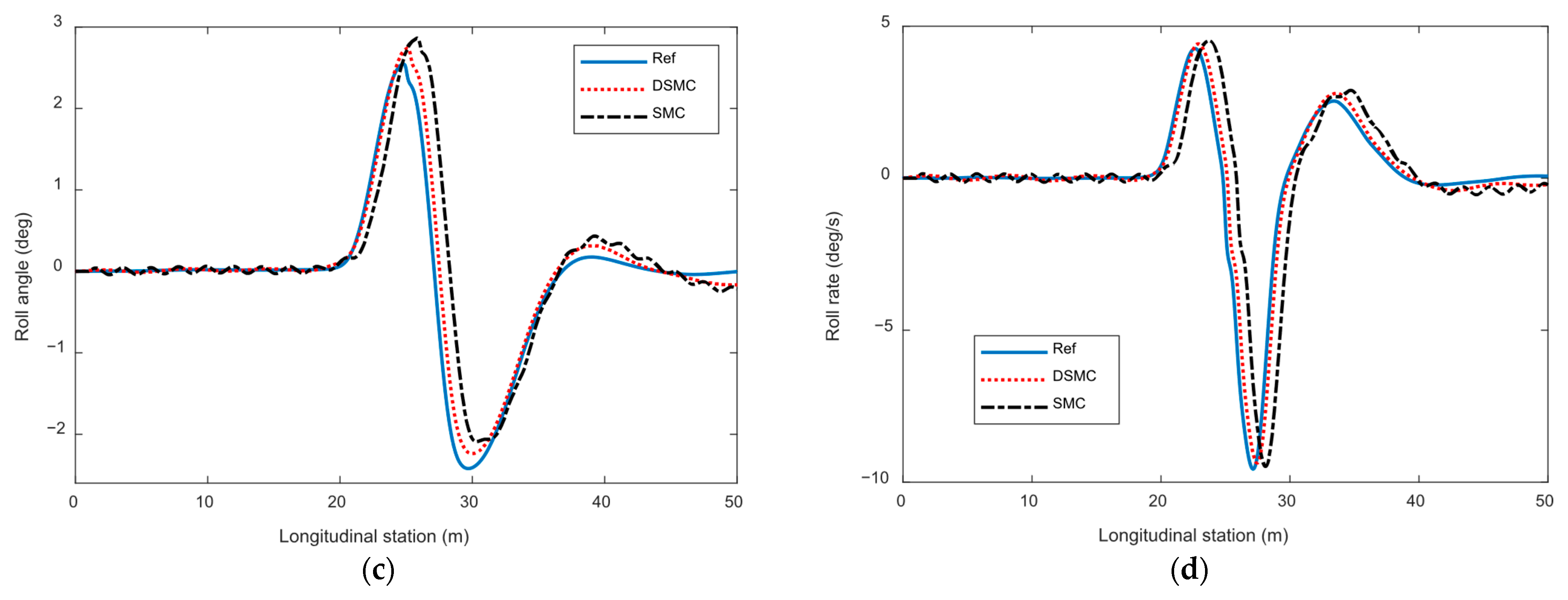
During the lane-change process, the integrated stability control effect of vehicle lateral roll is shown in Figure 7. In order to independently reflect the effects of different control algorithms and obtain reliable reference values, in the simulation test, a trajectory-tracking controller was first established only in the Simulink model and the required front-wheel steering angle for control was obtained. Input the obtained front-wheel steering angle into the CarSim model and use the stability control module built-in in the model to achieve the stability requirements of the vehicle. Collect the vehicle-state variables under lane-changing conditions and use them as reference values. In this way, the stability control effect of the vehicle after the intervention of the designed control algorithm can be effectively reflected. As shown in the figure, compared with DSMC, the vehicle yaw rate under SMC algorithm has the problem of tracking control lag, and the vehicle yaw rate under SMC algorithm exhibits a certain degree of oscillation fluctuation. In contrast, the vehicle yaw rate curve under DSMC algorithm is smoother, which reflects that the introduced double-power convergence law can effectively improve the inherent oscillation problem of conventional SMC algorithm and switching control law. In the vehicle center of the mass lateral angle curve, the control results under DSMC algorithm are closer to the reference value, and its convergence speed and ability to suppress amplitude oscillations are more prominent. In contrast, under the SMC algorithm, the oscillation phenomenon of the vehicle’s center-of-mass sideslip angle curve is more obvious, with the maximum value of the center-of-mass sideslip angle approaching 0.4 degrees. The convergence speed of the state amplitude is slower, and the overall deviation degree of the amplitude is also greater. The control results of vehicle roll angle and roll-angle speed also showed the same trend. As shown in the figure, the vehicle’s roll angle and roll-angle speed also show a sharp increase and rapid fluctuation during lane changing and vehicle turning. At this point, there is a more significant lack of tracking capability and amplitude oscillation deviation in the tracking control results of SMC. In contrast, the vehicle-state curve under DSMC algorithm has higher smoothness, and the fluctuation amplitude of vehicle roll angle and roll-angle velocity is effectively suppressed, which helps to further improve vehicle stability. On the premise of theoretical analysis, combined with the simulation results, the designed control system has a stable equilibrium point, which ensures the gradual stability of the system control effect. The introduction of double-power convergence law makes the system have fast reaching characteristics when it is far from the equilibrium point, and can achieve smooth convergence when it is close to the equilibrium point. This property effectively solves the chattering problem of traditional sliding-mode control.

The high-speed core scenario of the strategy is locked in the typical high lateral excitation and high-speed coupling condition of “highway lane change emergency obstacle avoidance”, and its longitudinal speed range covers the daily high-speed cruise to the section close to the upper limit of vehicle dynamics. In this scenario, the comprehensive performance of trajectory-tracking accuracy and lateral roll stability needs to meet the criteria of “no significant delay and no visible oscillation”. When the vehicle can finish track tracking continuously and smoothly in the process of high-speed lane changing, and the roll motion and yaw response do not have secondary fluctuations that can be perceived by the driver and passengers, it can be determined that the strategy has sufficient conditions to serve as the engineering benchmark at the current hardware level. For extreme cases beyond the above scene boundary, the strategy will automatically switch to the safety degradation mode with “maintaining driving stability” as the priority, instead of continuing to pursue centimeter-level tracking accuracy.

In the process of control algorithm verification, the significance of quantitative statistical control error is that it can convert the qualitative judgment of performance into a comparable quantitative objective index, so as to provide a more accurate argument for the effectiveness of the algorithm. Through the statistics of the average error and root mean square error of key state variables such as lateral deviation, heading deviation and yaw rate, vehicle sideslip angle, roll angle and roll rate, the specific performance of the proposed control law in providing control effect can be further revealed. Then, the error average (e_a) and error root mean square (e_r) can be denoted as

$$\begin{array}{c}{e}_a={\displaystyle \frac{1}{N}}{\displaystyle \sum _{i=1}^N\left({\widehat{x}}_i-x_i\right)}\\ e_r=\sqrt{{\displaystyle \frac{1}{N}}{\displaystyle \sum _{i=1}^N{\left({\widehat{x}}_i-x_i\right)}^2}}\end{array}$$

(44)

where N is sampling amount, $x_i$ denotes referenced value, ${\widehat{x}}_i$ represents estimated value. The quantitative comparison results of e_AVE and e_RMSE are listed in

Table 2. Quantitative comparison results of e_AVE and e_RMSE.

Index	Algorithm	Lateral Deviation	Heading Error	Yaw Rate	Vehicle Sideslip Angle	Roll Angle	Roll Rate
eAVE	SMC	0.3944	0.6284	0.8904	0.0356	0.1395	0.2233
	HSMC/DSMC	0.0779	0.1265	0.6721	0.0189	0.0816	0.1783
eRMSE	SMC	0.5684	0.5377	0.2353	0.2295	0.2387	0.2971
	HSMC/DSMC	0.3907	0.3692	0.1899	0.1638	0.1606	0.1726

. From the overall comparative data, the proposed HSMC/DSMC control algorithm is superior to the traditional SMC in all six indicators, and the error reduction degree presents the hierarchical characteristics of significant lateral heading and moderate yaw roll. Specifically, in the two channels that directly affect the trajectory-tracking accuracy, lateral deviation, and heading error, the average value and root mean square of the error are significantly suppressed, indicating that the combination of high-order sliding-mode surface and double-power convergence law significantly weakens the trajectory lag and overshoot, and verifies the effectiveness of chattering suppression and finite-time convergence. In terms of the state variables related to stability, such as yaw rate, vehicle sideslip angle, roll angle and its angular velocity, the error is also reduced, but the amplitude is relatively mild, reflecting the trade-off between steady-state smoothness and dynamic response achieved by the lateral roll integrated control: it neither excessively inhibits the necessary yaw maneuver, but also effectively suppresses the roll oscillation. In summary, the collaborative strategy not only maintains the naturalness of vehicle motion, but also reduces the trajectory error and stability fluctuation, which provides a quantitative basis for pervasive control for most operating conditions.

5. Conclusions

(1) A lateral-roll coupling dynamic model and trajectory error model were established, and real-time accurate estimation of key unmeasurable states was achieved through EKF, solving the problems of difficult state acquisition and insufficient measurement accuracy in high dynamic processes.

(2) The proposed HSMC trajectory-tracking algorithm embeds the high-order derivatives of the sliding surface into the integral chain and uses virtual control variables to smooth the switching signal, fundamentally suppressing the chattering phenomenon of traditional sliding mode and ensuring that the system converges to the sliding-mode set within a finite time, significantly improving trajectory-tracking accuracy and ride comfort.

(3) The designed DSMC integrated lateral-roll controller is based on the double-power law of convergence, and adjusts the lateral and roll control torques online according to the estimated state, taking into account both fast convergence and steady-state smoothing requirements, achieving coordinated stable control of vehicle lateral-roll motion.

(4) Finally, based on the CarSim–Simulink joint simulation platform, the proposed strategy was validated in a high-speed lane-changing scenario with a vehicle speed of 20 m/s and a road adhesion coefficient of 1.0. The results show that compared with conventional sliding mode, HSMC reduces the maximum lateral deviation from 1.5 m to 0.25 m, reduces the peak heading deviation from 3 deg to within 1 deg, and has no visible chattering. Compared to standard Kalman filtering, EKF suppresses the delay in estimating results during state transitions. Under DSMC control, the oscillation amplitude of yaw rate and roll-angle velocity significantly decreases, and the overshoot of the center of mass roll angle is almost eliminated. The proposed method is significantly superior to traditional methods in terms of tracking accuracy, response speed, and stability, verifying the effectiveness and engineering feasibility of the method.

(5) In the future research work, the influence of parameter uncertainty, actuator saturation and complex road adhesion conditions on the control effect will be further considered from the perspective of model and algorithm. At the model level, it is planned to introduce the coupling term of nonlinear tire force model and aerodynamics, and dynamically correct the sideslip stiffness and wind load disturbance through the parameter online identification mechanism, so as to break through the working condition boundary of the current linear hypothesis; at the algorithm level, the high-order sliding mode and double-power sliding-mode framework are extended to a multi-stage adaptive structure. According to the road adhesion level and the vehicle state, the real-time switching gain is obtained, and the event trigger mechanism is introduced to reduce the computational load, so as to ensure the implement ability in the vehicle-embedded platform. In addition, for the problem of model mismatch and constraint coupling, the improved model predictive control can be studied. Through online linearization error correction and rolling time-domain adaptive weight, model predictive control can maintain the advantages of explicit constraint processing and reduce the dependence on accurate models; its output will form a two-tier architecture with the sliding-mode controller. The upper-model predictive control is responsible for global trajectory planning and constraint feasible region determination. The lower sliding mode can quickly compensate the model error and external disturbance to realize the complementarity of calculation accuracy and real-time performance. Secondly, for high-dimensional nonlinear dynamics and unknown disturbance scenarios, the deep reinforcement learning method will be explored and the end-to-end control strategy will be learned online; at the same time, a secure filter layer is designed to limit the reinforcement learning output to the attraction region of the sliding-mode surface, ensuring that the stability constraint can be met at the initial stage of training.

References

1. Zhao, W.Q. Real-Time Model Predictive Control of Path-Following for Autonomous Vehicles Towards Model Mismatch and Uncertainty. Control Eng. Pract. 2024, 142, 105678. [Google Scholar] [CrossRef]
2. Cui, K.; He, J.; Yao, X.; Gu, X. Adaptive Model Predictive Control Based on Stability Index for Path Tracking of Autonomous Vehicles Considering Model Error. Proc. Inst. Mech. Eng. Part C J. Mech. Eng. Sci. 2024, 238, 9372–9396. [Google Scholar] [CrossRef]
3. Hu, J.; Liu, Y.; Xiao, F.; Lin, Z.; Deng, C. Coordinated Control of Active Suspension and DYC for Four-Wheel Independent Drive Electric Vehicles Based on Stability. Appl. Sci. 2022, 12, 11768. [Google Scholar] [CrossRef]
4. Napolitano Dell’Annunziata, G.; Ruffini, M.; Stefanelli, R.; Adiletta, G.; Fichera, G.; Timpone, F. Four-Wheeled Vehicle Sideslip Angle Estimation: A Machine Learning-Based Technique for Real-Time Virtual Sensor Development. Appl. Sci. 2024, 14, 1036. [Google Scholar] [CrossRef]
5. Li, H.; Li, B.; Yang, H.; Mu, C. Nonlinear Model Predictive Control for Time-Optimal Turning Around of an Autonomous Vehicle Under Steering Lag. IEEE/ASME Trans. Mechatron. 2025, 30, 577–586. [Google Scholar] [CrossRef]
6. Feng, H.; Zhou, Y.; Li, S.; Cheng, G.; Ma, S.; Li, Y. Adaptive Backstepping Control with Time-Delay Compensation for MR-Damper-Based Vehicle Seat Suspension. Actuators 2025, 14, 178. [Google Scholar] [CrossRef]
7. Zhao, Z.; Zhang, L.; Ding, X.; Zhang, Z.; Li, S.; Gu, L. Integrated Active Suspension and Anti-Lock Braking Control for Four-Wheel-Independent-Drive Electric Vehicles. Chin. J. Mech. Eng. 2024, 37, 20. [Google Scholar] [CrossRef]
8. Yang, Y.; Liu, C.; Lai, S.K.; Chen, Z.; Chen, L. Frequency-dependent equivalent impedance analysis for optimizing vehicle inertial suspensions. Nonlinear Dyn. 2024, 113, 9373–9398. [Google Scholar] [CrossRef]
9. Boada, B.L.; Viadero-Monasterio, F.; Zhang, H.; Boada, M.J.L. Simultaneous Estimation of Vehicle Sideslip and Roll Angles Using an Integral-Based Event-Triggered H∞ Observer Considering Intravehicle Communications. IEEE Trans. Veh. Technol. 2023, 72, 4411–4425. [Google Scholar] [CrossRef]
10. Liu, Y.; Gao, H. Stability, scalability, speedability, and string stability of connected vehicle systems. IEEE Trans. Syst. Man Cybern. Syst. 2021, 52, 2819–2832. [Google Scholar] [CrossRef]
11. Jiang, Y.; Meng, H.; Chen, G.P.; Yang, C.N.; Xu, X.J.; Zhang, L.; Xu, H.J. Differential-steering based path tracking control and energy-saving torque distribution strategy of 6WID unmanned ground vehicle. Energy 2022, 254, 124209. [Google Scholar] [CrossRef]
12. Lee, J.E.; Kim, B.W. A Novel Adaptive Non-Singular Fast Terminal Sliding Mode Control for Direct Yaw Moment Control in 4WID Electric Vehicles. Sensors 2025, 25, 941. [Google Scholar] [CrossRef] [PubMed]
13. Wang, X.; Chen, T.; Lu, J. Longitudinal Tire Force Estimation Method for 4WIDEV Based on Data-Driven Modified Recursive Subspace Identification Algorithm. Algorithms 2025, 18, 409. [Google Scholar] [CrossRef]
14. Chen, X.; Zhang, W.; Bai, H.; Jiang, R.; Ding, H.; Wei, L. A Sigmoid-Based Car-Following Model to Improve Acceleration Stability in Traffic Oscillation and Following Failure in Free Flow. IEEE Trans. Intell. Transp. Syst. 2024, 25, 9039–9057. [Google Scholar] [CrossRef]
15. Meng, D.; Chu, H.; Tian, M.; Gao, B.; Chen, H. Real-Time High-Precision Nonlinear Tracking Control of Autonomous Vehicles Using Fast Iterative Model Predictive Control. IEEE Trans. Intell. Veh. 2024, 9, 3644–3657. [Google Scholar] [CrossRef]
16. Liang, J.; Tian, Q.; Feng, J.; Pi, D.; Yin, G. A Polytopic Model-Based Robust Predictive Control Scheme for Path Tracking of Autonomous Vehicles. IEEE Trans. Intell. Veh. 2024, 9, 3928–3939. [Google Scholar] [CrossRef]
17. Wan, Z.; Xu, C.; Li, B.; Li, Y.; Ye, F. Trajectory Tracking Method of Four-Wheeled Independent Drive and Steering AGV Based on LSTM-MPC and Fuzzy PID Cooperative Control. Electronics 2025, 14, 2000. [Google Scholar] [CrossRef]
18. Huang, K.; Wei, K.; Li, F.; Yang, C.; Gui, W. LSTM-MPC: A Deep Learning Based Predictive Control Method for Multimode Process Control. IEEE Trans. Ind. Electron. 2022, 70, 11544–11554. [Google Scholar] [CrossRef]
19. Guo, N.; Zhang, X.; Zou, Y.; Lenzo, B.; Du, G.; Zhang, T. A Supervisory Control Strategy of Distributed Drive Electric Vehicles for Coordinating Handling, Lateral Stability, and Energy Efficiency. IEEE Trans. Transp. Electrif. 2021, 7, 2488–2504. [Google Scholar] [CrossRef]
20. Hua, X.; Xiang, K.; Cheng, X.; Ning, X. An Adaptive Compound Control Strategy of Electric Vehicles for Coordinating Lateral Stability and Energy Efficiency. Appl. Sci. 2025, 15, 3347. [Google Scholar] [CrossRef]
21. Liu, W.; Zhang, J.; Ma, R.; He, C. Cascade-Free Predictive Wheel Slip Control with Discrete-Valued Inputs for Automotive Hydraulic Anti-lock Braking Systems. IEEE Trans. Transp. Electrif. 2024, 11, 6048–6059. [Google Scholar] [CrossRef]
22. Lee, J.E.; Kim, B.W. Improving Direct Yaw-Moment Control via Neural-Network-Based Non-Singular Fast Terminal Sliding Mode Control for Electric Vehicles. Sensors 2024, 24, 4079. [Google Scholar] [CrossRef] [PubMed]
23. Tao, Y.; Ge, C.; Feng, H.; Xue, H.; Yao, M.; Tang, H.; Liao, Z.; Chen, P. A novel approach for adaptively separating and extracting compound fault features of the in-wheel motor bearing. ISA Trans. 2025, 159, 337–351. [Google Scholar] [CrossRef] [PubMed]
24. Micheli, F.; Bersani, M.; Arrigoni, S.; Braghin, F.; Cheli, F. NMPC Trajectory Planner for Urban Autonomous Driving. Veh. Syst. Dyn. 2023, 61, 1387–1409. [Google Scholar] [CrossRef]
25. Chen, J.; Wang, R.; Liu, W.; Sun, D.; Jiang, Y.; Ding, R. A Review of Recent Advances in Roll Stability Control in On-Road and Off-Road Vehicles. Appl. Sci. 2025, 15, 5491. [Google Scholar] [CrossRef]
26. Picotti, E.; Mion, E.; Libera, A.D.; Pavlovic, J.; Censi, A.; Frazzoli, E.; Beghi, A.; Bruschetta, M. A Learning-Based Nonlinear Model Predictive Controller for a Real Go-Kart Based on Black-Box Dynamics Modeling Through Gaussian Processes. IEEE Trans. Control Syst. Technol. 2023, 31, 2034–2047. [Google Scholar] [CrossRef]
27. Pinho, J.; Costa, G.; Lima, P.U.; Ayala Botto, M. Learning-Based Model Predictive Control for Autonomous Racing. World Electr. Veh. J. 2023, 14, 163. [Google Scholar] [CrossRef]
28. Manzano, J.M.; Limon, D.; de la Peña, D.M.; Calliess, J.P. Robust learning-based MPC for nonlinear constrained systems. Automatica 2020, 117, 108948. [Google Scholar] [CrossRef]
29. Feng, H.; Tao, Y.; Feng, J.; Zhang, Y.; Xue, H.; Wang, T.; Xu, X.; Chen, P. Fault-tolerant collaborative control of four-wheel-drive electric vehicle for one or more in-wheel motors’ faults. Sensors 2025, 25, 1540. [Google Scholar] [CrossRef]
30. Zhang, Z.; Ding, H.; Guo, K.; Zhang, N. A Hierarchical Control Strategy for FWID-EVs Based on Multi-Agent with Consideration of Safety and Economy. Energies 2022, 15, 9112. [Google Scholar] [CrossRef]
31. Qi, G.X.; Yue, M.; Shangguan, J.; Guo, L.; Zhao, J. Integrated Control Method for Path Tracking and Lateral Stability of Distributed Drive Electric Vehicles with Extended Kalman Filter-Based Tire Cornering Stiffness Estimation. J. Vib. Control 2024, 30, 2582–2595. [Google Scholar] [CrossRef]
32. Wang, Z.J.; Zhou, X.Y.; Wang, J.M. Extremum-Seeking-Based Adaptive Model-Free Control and Its Application to Automated Vehicle Path Tracking. IEEE-ASME Trans. Mechatron. 2022, 27, 3874–3884. [Google Scholar] [CrossRef]
33. Li, J.; Wang, F.; Guo, W.; Zhou, Z.; Miao, S.; Chen, T. Hierarchical Coordination Control of Distributed Drive Intelligent Vehicle Based on TSMPC and Tire Force Optimization Allocation. Algorithms 2025, 18, 508. [Google Scholar] [CrossRef]
Figure 1. Vehicle dynamic model. (a) Lateral dynamic model; (b) vertical dynamic model.
Wevj 16 00524 g001
Figure 2. Vehicle trajectory-tracking model.
Wevj 16 00524 g002
Figure 3. Architecture of overall coordination control strategy.
Wevj 16 00524 g003
Figure 4. Comparison of vehicle trajectory-tracking effects. (a) Vehicle trajectory; (b) heading angle.
Wevj 16 00524 g004
Figure 5. Comparison of vehicle trajectory-tracking control errors. (a) Lateral deviation; (b) heading error.
Wevj 16 00524 g005
Figure 6. Comparison of vehicle-state estimation performance: (a) vehicle sideslip angle, (b) roll angle, (c) roll rate.
Wevj 16 00524 g006
Figure 7. Comparison of the integrated lateral-roll stability control effects of vehicle. (a) Vehicle yaw rate, (b) vehicle sideslip angle, (c) roll angle, (d) roll rate.
Wevj 16 00524 g007aWevj 16 00524 g007b