Empirical Energy Consumption Estimation and Battery Operation Analysis from Long-Term Monitoring of an Urban Electric Bus Fleet

Abstract

Electric buses are key in the strategy towards a greenhouse-gas-neutral fleet. However, their restrictions in terms of range and refueling as well as their increased price point present new challenges for public transport companies. This study aims to address, based on real-world operational data, how energy consumption and charging behavior affect battery aging and how operational strategies can be optimized to extend battery life under realistic conditions. This article presents an energy consumption analysis with respect to ambient temperatures and average vehicle speed based exclusively on real-world data of an urban bus fleet, providing a data foundation for range forecasting and infrastructure planning optimized for public transport needs. Additionally, the State of Charge (SOC) window during operation and vehicle idle time as well as the charging power were analyzed in this case study to formulate recommendations towards a more battery-friendly treatment. The central research question is whether battery-friendly operational strategies—such as reduced charging power and lower SOC windows—can realistically be implemented in daily public transport operations. The impact of the recommendations on battery lifetime is estimated using a battery aging model on drive cycles. Finally, the reduction in CO₂ emissions compared to diesel buses is estimated.

1. Introduction

Among the 35,579 buses sold in the European Union (EU) throughout the year 2024, 18.5% of them were electrically chargeable vehicles [1]. Although diesel powered vehicles still make up the majority of sold buses (63.1%), fully electric buses are no longer a niche market, especially with EU climate goals set to reduce greenhouse gas emissions by at least 55% by 2030 compared to 1990 levels [2].

However, with the often two to three times higher initial vehicle cost compared to internal combustion engine (ICE) buses, infrastructure investments for charging stations, and operation restrictions regarding vehicle range and downtime for charging, it is economically challenging to justify the transition to a fully electric bus fleet. Economic feasibility is usually evaluated by a total cost of ownership (TCO) study, which covers the individual demands and constraints of public transport companies [3,4,5,6].

By long-term monitoring of battery-electric bus (BEB) fleets, important operational aspects that contribute to overall cost and performance can be assessed in detail. These include the specific energy consumption (SEC)—in kWh/km—which directly relates to operational energy costs and indicators of battery usage that inform potential impacts on battery lifetime. While a full TCO analysis is beyond the scope of this study, insights into these two factors can support such evaluations. For instance, energy consumption data helps assess the feasibility of specific circulations under varying ambient conditions, while battery-friendly operation strategies may reduce long-term degradation, indirectly contributing to lower total costs over time.

1.1. Energy Consumption Estimation of BEBs

Accurately estimating the energy consumption of BEBs is essential for feasibility studies aimed at transitioning urban transit systems from conventional to electric propulsion. A common but overly simplistic method is to assume a constant specific energy consumption value (e.g., 1.5 kWh/km), applying a linear relationship between energy use and distance traveled [7,8]. This approach neglects critical variables such as route topology, vehicle load, and auxiliary energy demands, particularly for heating and air conditioning.

To address these limitations, a variety of advanced methodologies have been proposed in the literature, including physical modeling, regression-based techniques, machine learning algorithms, and hybrid approaches that integrate multiple methods [9,10]. For instance, Gallet et al. [11] developed a longitudinal dynamics model that estimates energy demand without requiring detailed drive cycle data. While this method reduces input data requirements, it may compromise predictive accuracy compared to more detailed approaches.

Abdelaty et al. [12] introduced a multivariate regression model calibrated using 120 real-world drive cycles. Their findings indicate that energy consumption can vary substantially—ranging from 1.109 to 3.05 kWh/km—depending on vehicular, operational, topographical, and environmental parameters.

An alternative and widely adopted approach involves vehicle simulation models, which utilize detailed drive cycles and comprehensive vehicle parameterization to estimate energy use with high fidelity [7,13,14]. More recently, data-driven techniques, particularly artificial neural networks (ANNs), have gained traction. These models are trained on large datasets of operational bus data and are capable of capturing complex nonlinear relationships between influencing factors and energy consumption [15,16].

1.2. Battery-Friendly Operation

It is beyond the scope of this paper to address the details of electrochemical processes responsible for battery degradation, which are extensively studied in the literature [17,18,19,20,21]. On a more general level, it is common to differentiate into calendric and cyclic aging when discussing battery degradation [19,20].

Calendric aging is exponentially increasing with cell temperature and voltage [22]. It is therefore recommended to store a battery at relatively low cell voltage and therefore low SOC (e.g., 30%). Depending on the specific cell chemistry, additional degradation processes may modify this general behavior, e.g., accelerated aging in a certain SOC range [23,24,25]. Storing an NMC battery at around 30% SOC can reduce the effects of calendric aging by a factor of two compared to storing at near 100% SOC [26,27].

When discussing cyclic aging, the SOC operating window and the charge/discharge rate are of importance. Operating a battery with a low DoD but high SOC level, close to 80–100%, may result in about 40% higher capacity degradation compared to, e.g., 40–60% [28]. For battery operation, a low DoD centered at around 50% SOC or lower is ideal with details varying by cell type [28,29,30]. The charge and discharge rate also influences cyclic battery aging as charging at high currents and suboptimal battery temperatures may result in faster degradation [31,32,33,34,35].

Based on the results of battery degradation studies, general battery operating rules can be formulated, positively impacting battery degradation, i.e., the reduction in battery capacity and (maximum) power output:

• Operate at low Depth of Discharge (DoD) cycles centered at about 50% SOC or lower with frequent charging;
• Operate at near room temperature and store at a low temperature;
• Keep the battery at a low SOC level when storing for longer periods of time (e.g., 30%);
• Avoid high SOC states (typically, degradation is highest at 100% SOC due to higher cell voltage);
• Charge at low power using C-rates below 2 C, where the C-rate refers to the rate at which a battery is charged or discharged relative to its capacity (e.g., 1 C means a full charge or discharge in one hour).

Note that these rules are general best practices, and the ideal battery operation may be adjusted based on the exact composition. Also, these rules are formulated solely from the perspective of battery-friendly operation. Depending on the use case, it may not be economically feasible to (strictly) follow these rules as they reduce flexibility and increase downtime for charging.

1.3. Research Contribution of This Study

This study presents several key findings regarding the operation of a battery electric urban bus fleet. Solely based on vehicle monitoring data of a bus fleet for about 2.5 years, the SEC is analyzed with respect to the ambient temperature and the average speed allowing for easy-to-use range and cost estimation. The given values are to be interpreted as the round-trip SEC for urban drive cycles with zero elevation difference between the start and end point.

While various modeling techniques—ranging from physics-based simulations to statistical and machine learning approaches—exist for estimating vehicle energy consumption, this study deliberately follows a purely empirical and data-driven strategy. For instance the acceleration profile, although not explicitly modeled, is inherently driver-specific and varies significantly across urban bus operations. Its influence is indirectly captured through average speed, which correlates with stop-and-go intensity and dwell times and is further reflected in the observed spread of the specific energy consumption (SEC), particularly within the 10th to 90th percentile range. This approach ensures robust and interpretable results without overfitting to driver behavior or specific operating patterns, supporting generalizable insights for fleet-level operational planning.

To address the rules of battery-friendly vehicle operation, the SOC level during operation and idle time as well as the charging power are analyzed. Based on the analysis of the current fleet operation, recommendations for an increased battery lifetime are given. The impact on bus delays and battery lifetime of those recommendations are then evaluated by estimating the additional charge time and applying a battery aging model to an original and an optimized drive cycle. Finally, the reduction in CO₂ emissions compared to diesel buses is estimated in this study.

2. Methods

2.1. Overview over Bus Fleet and Signal Set

A mixed fleet of solo and articulated fully battery-electric buses has been monitored starting mid-2022 (the exact starting date varies by bus) until 28 February 2025. The total distance and number of operating days, as well as information about the battery, are given in

Table 1. Overview of the monitored bus fleet (rotated). The number of operating days was identified within the energy consumption analysis (see Section 2.2).

Attribute	Solo Bus, 12 m	Articulated Bus, 18 m
Curb Weight including battery (t)	14.5	21.9
Engine Power (Peak/Continuous) (kW)	250/125	250/125
Total Battery Capacity (kWh)	258	322.5
Battery Chemistry	NMC	NMC
Total Monitored Distance (Tkm)	372.6	3029.3
Total Days in Monitoring	2030	16,033
Total Operating Days	1413	11,564

. The difference between the Total Operating Days and Total Days in Monitoring originates from filtering out days with data gaps and inconsistencies as well as idle times where the bus was parked at a depot. All vehicles included in the monitoring campaign were nearly new at the onset of data collection, with odometer readings below 1000 km at the beginning of the observation period.

Relevant signals from the OEM cloud service were long-time stored and evaluated using the Cloud2Cloud capabilities of the IVImon platform [36]. Relevant signals and their time resolutions are listed in

Table 2. Vehicle signals and their time resolution used for evaluations. Temperature values are obtained from open-meteo [37].

Signal	Unit	Time Resolution
Battery Power	kW	100 ms
Battery Current	A	100 ms
State of Charge (SOC)	%	On value-change
Vehicle Speed	km/h	100 ms
Total mileage	km	1 s
Vehicle weight	kg	200 ms
GPS altitude	m	Few seconds (varying)
Ambient Temperature	°C	1 h

.

Due to data gaps and irregularities in the temperature signal at an air vent, that could in principle be used to monitor the ambient temperature, hourly temperature values from open-meteo were taken for the evaluation [37].

2.2. Energy Consumption Analysis

Long-term monitoring allows for analyzing the energy consumption at different operational conditions and using this data for future disposition planning. The benefit of this approach is the data-driven nature without the need for extensive modeling as studied in the literature (see Section 1.1). There are several influencing factors regarding the energy consumption of an electric vehicle for a specific trip. Figure 1 presents a scheme of the most important indirect and direct factors considered in this paper impacting the SEC.

The speed profile is of great importance as many acceleration and deceleration processes during a trip, like in stop-and-go traffic, result in higher energy consumption. It is mainly influenced by the bus driver and regulatory factors like bus lanes and traffic lights. Especially at higher speeds, wind resistance leads to a higher SEC as well, due to the quadratic influence of the vehicle speed to drag forces. The speed signal is also used for trip detection in the following way: A trip starts as soon as the speed signal is above zero and ends when the signal reaches zero and the time at rest is longer than four minutes. This prevents stop-and-go traffic and breaks at bus stops from ending the trip time period. Only trips that are longer than ten minutes are evaluated for the energy consumption analysis to prevent short maneuvers and test drives from influencing the results. For each detected trip, the average speed is calculated by dividing the total distance by the trip duration. In the context of urban buses, a lower average speed mostly indicates a longer rest time at stations and traffic lights and more stop-and-go traffic in general.

An example dataset for an operational day of a bus is shown in Figure 2. Panel (a) shows the vehicle speed signal for one day of operation. In total, 11 individual trips are identified from that signal; the beginning and end of such trips are marked with a green and red vertical line, respectively.

While the ambient temperature plays a big role in energy consumption due to higher secondary consumers like heating, as well as higher power draw of the battery thermal management, wind conditions are considered negligible for urban bus speed profiles within this paper.

Figure 2b–g show important quantities of one detected trip indicated by the lines connecting subplots (a) and (b). The battery power is shown in panel (e), where negative values indicate power drawn from the battery, and positive values show energy recuperation from braking and the beginning of a charging process at around 15:47. The following quantities were evaluated for each trip: The distance value can be directly taken from the vehicle odometer signal by subtracting the values at the end and start of the trip. Dividing the distance by the trip duration directly yields the average speed of the trip. The energy is calculated from the mean value of the battery power signal, available with a time precision of 100 ms, multiplied by the trip duration. The ambient temperature is taken from the hourly open-meteo dataset by finding the closest timestamp to the trip after half of the trip duration. The results for the 11 trips identified in Figure 2a are listed in

Table 3. Evaluated values for the 11 individual trips for the dataset shown in Figure 2.

Trip Nr.	Distance (km)	Energy (kWh)	Average Speed (km/h)	Ambient Temperature (°C)	Average Vehicle Weight (t)	Elevation Difference (m)	SEC (kWh/km)
1	15.58	30.86	21.52	0.8	22.62	32.0	1.98
2	20.73	53.75	20.47	0.8	24.26	113.0	2.59
3	20.61	36.68	19.60	2.4	23.87	−124.3	1.78
4	20.72	43.52	20.10	6.8	24.58	123.9	2.10
5	20.60	25.56	20.02	8.3	24.03	−117.6	1.24
6	20.70	47.40	19.58	9.8	24.22	118.3	2.29
7	20.58	31.84	19.62	10.3	23.60	−113.8	1.55
8	20.68	45.79	19.41	10.1	23.68	111.0	2.21
9	20.51	33.02	18.60	9.9	24.21	−109.1	1.61
10	20.75	45.64	19.61	7.4	23.25	108.1	2.20
11	8.17	7.58	23.33	7.4	22.47	−108.2	0.93

.

The elevation profile influences the trip energy consumption heavily. When looking at the values given in Table 3, trips 2 to 10 all have nearly identical distances. However, subsequent trips have opposite elevation differences due to the same route being driven back and forth resulting in trips 2, 4, 6, 8, and 10 having up to 85% higher SEC compared to the trips 3, 5, 7, and 9. To mostly eliminate the influence of the elevation profile of individual trips, as well as reduce the impact of outliers, a daily grouping of the trips is performed.

For the daily grouping, the distance and energy values of all trips during an operating day and of an individual bus are summed up. New energy consumption and average speed values are calculated from the summed-up distance, energy, and trip duration values. To calculate daily averaged temperatures and vehicle weights and account for the possibility of trips with largely different distances, the individual values are weighted by the trip distances:

$$\overline{x}={\displaystyle \frac{1}{{\sum }_{j=1}^n{d}_j}}\sum _{i=1}^n{x}_i{d}_i$$

(1)

Here, x is either the ambient temperature T or the vehicle weight m, $\overline{x}$ is the daily average value, $x_i$ is the average value of trip i, $d_i$ is the distance of trip i, and n is the total number of trips detected during the day of operation. The daily grouping of the individual trip values given in Table 3 results in the values given in

Table 4. Daily grouped trip values evaluated from the individual trip values given in Table 3 and shown in Figure 1.

Distance (km)	Energy (kWh)	Average Speed (km/h)	Distance- Weighted Average Temperature $\overline{\mathit{T}}$ (°C)	Distance- Weighted Average Vehicle Weight $\overline{\mathit{m}}$ (t)	SEC (kWh/km)
209.61	401.64	19.91	6.83	23.81	1.92

.

The procedure was conducted for all operating days for each bus without discrepancies in the dataset, such as nonphysically low or large vehicle weight, with more than 50 km daily distance driven, resulting in 1413 data points for the solo buses and 11,564 data points for articulated buses. Histograms of the number of data points with respect to average speed, distance-weighted average temperature, and vehicle weight are shown in Figure 3.

2.3. Usage Analysis on SOC Levels and Charging Power

In this study, the driven kilometers of electric buses within specific ranges of battery SOC are analyzed by dividing the SOC into 20 intervals ranging from 0% to 100% in increments of 5%. The total kilometers driven within each SOC bin are aggregated for each day and vehicle, providing an overview of the relationship between battery state and distance traveled.

In order to evaluate the distribution of SOC during the idle time of electric buses, a series of data processing functions is employed. Therefore, the SOC, vehicle speed, and current flow signals as well as the odometer signal are used. The odometer signal is used to detect data gaps where the vehicle was operated. Such data gaps with an odometer signal discrepancy were discarded and therefore not counted towards vehicle idle time. Then, the data was resampled to a 1 min frequency using interpolation methods to fill in missing values. Again, the SOC is divided into 20 intervals, and for each interval, the occurrences where the vehicles is stationary (speed equal to 0) and the battery current is below 1 A is counted, resulting in a dataset containing the amount of time (in minutes, later converted into days) each bus spent idle at varying SOC levels.

To assess the charged energy (in kWh) within different ranges of charging power (in kW), the battery power signal was used. Battery charging sections were identified by finding sections where the battery power was positive for longer than 1 min. The energy charged during each charging period was calculated using the trapezoidal integration method. The charging power was divided into intervals ranging from 0 to 300 kW in 10 kW increments, and the total energy charged for each interval is aggregated.

3. Results

3.1. Analysis of the Specific Energy Consumption

Based on the daily grouped dataset described in Section 2.2, the SEC was analyzed with respect to ambient temperature and average speed, the results of which are presented in Figure 4, with panels (a) and (b) for the solo and articulated buses, respectively. The data points are grouped into bins of speed and temperature ranges. The speed range is given in the legend of Figure 4; the temperature range is ±1 °C around the plotted data point. The points show the mean values of the energy consumption in kWh/km, with the shaded area of each curve ranging from the 10th and 90th percentile. Panels (c) and (d) show the 90th percentiles in separate plots as these values should be used for bus disposition planning.

In the ambient temperature range between 16 °C and 20 °C, the energy consumption is lowest for both types of buses and all average speed ranges. At temperatures above 22 °C, cabin climatization and battery thermal management (cooling) increase the SEC, e.g., by 13% when comparing 18 °C with 28 °C ambient temperature at the (18, 20) km/h speed range for articulated buses. At low temperature, the SEC increases until reaching a plateau at about 4 °C ambient temperature. This is due to an additional oil heater supporting cabin climatization and thus reducing battery energy consumption. Interestingly, the 90th percentiles for the articulated buses in panel (d) keep increasing until the lowest ambient temperature value in the dataset, with an exception at −4 °C and (18, 20) km/h due to only 16 daily grouped data points in that temperature and speed range. This may indicate that the additional oil heater is not always operating.

The deviations of the 10th and 90th percentile compared to the mean values are typically around 8% to 10%. There are several influencing factors on the SEC besides average speed and ambient temperature. One is the total vehicle weight, i.e., the difference between a (nearly) empty bus and a fully occupied one. However, when analyzing the daily distance-weighted average vehicle weight, the 10th and 90th percentile only differ by about 2% from the mean values. Since vehicle weight has a linear influence on the SEC, it should in turn result in deviations of about 2% [38]. The influence of the driver is probably the biggest factor as, at least for battery-electric passenger cars, an anticipatory driving style can reduce the energy consumption by up to 16% compared to aggressive driving and 7.1% compared to moderate driving behavior [39]. Higher average speed results in lower overall energy consumption which is attributed to less stop-and-go traffic due to traffic lights or congestion and shorter stopping times at stations. Thus, bus acceleration in cities by prioritization at traffic lights and setting up separate bus lanes is also a cost saving factor. The difference between the (18, 20) km/h and the (20, 22) km/h average speed intervals is about 0.05 kWh/km.

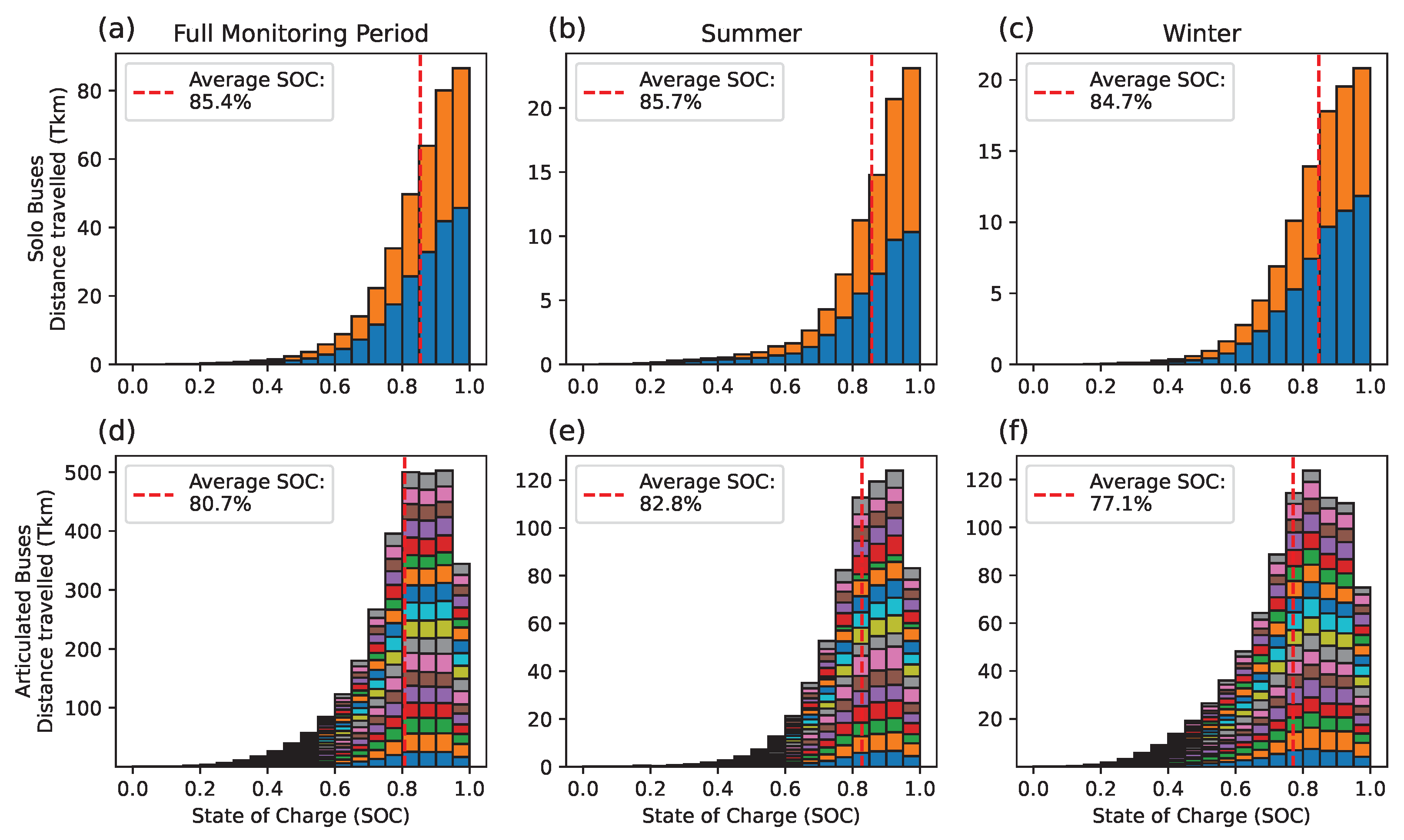
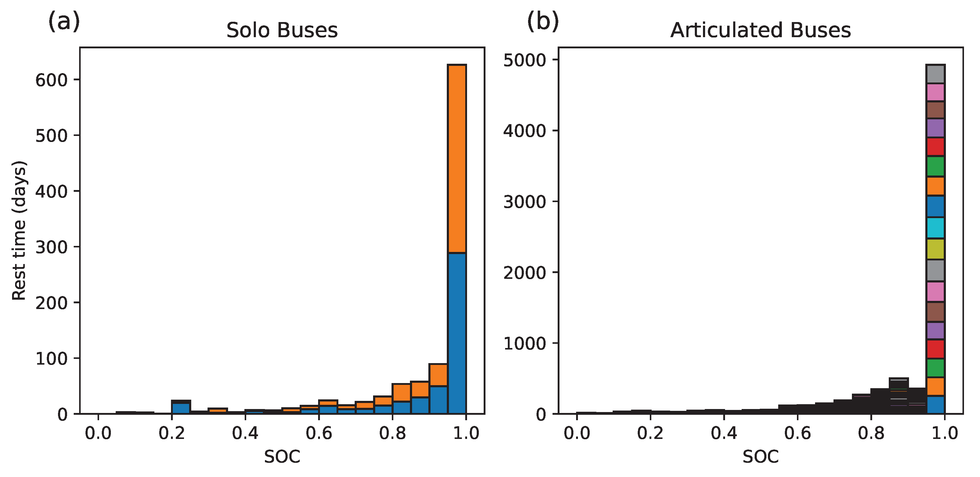
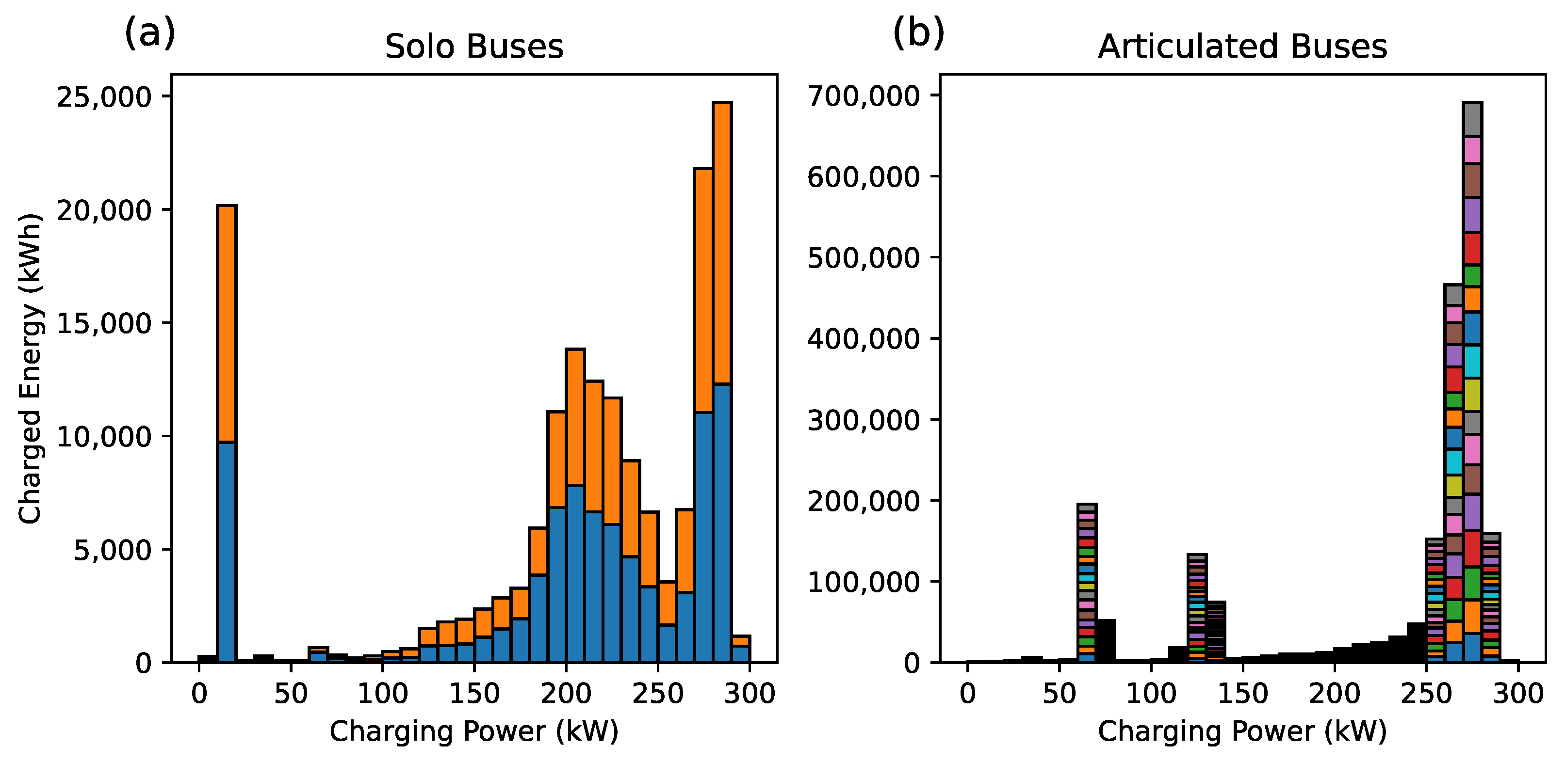
3.2. Analysis of Battery Operation

To address cyclic aging of the batteries in the electric bus fleet, the accumulated driven kilometers in each SOC range are presented in Figure 5. Panels (a), (b), and (c) show the results for solo buses in the entire time frame of the monitoring, in summer and in winter, respectively. Independently of the season, the bin with the highest driven distance is the one with the SOC level between 95% and 100%. Out of the total driven distance of 375,141 km, only 6617 km (or about 1.8%) were covered at SOC levels below 50%. In winter, the distance covered at an SOC level below 50% was only 1.5%, compared to 3.0% in summer. This may be due to precautions in winter. As already mentioned in rule 1 of the general battery-friendly operating rules (see Introduction), a low DoD centered at 50% or lower SOC are ideal for battery operation.

In Figure 5, panels (d), (e), and (f) present the same evaluation for the articulated buses. In terms of battery lifetime rules (see Section 1 “Introduction”), the articulated buses are operated more battery-friendly than the solo buses with a 5% lower average SOC over the full monitoring period. The 95% to 100% SOC bin is no longer the one with the highest driven distance. Instead, most kilometers are driven between 75% and 95% with a noticeable SOC level drop in winter compared to summer. During a regular operating day including opportunity charging, the battery is typically never charged up to 100% again. The total driven distance with an SOC level below 50% is equal to 3.5% (1.7% in summer; 6.3% in winter).

The most important arguments against lowering the SOC operating levels are usually added flexibility and reduced risk of running out of battery charge in case of a malfunction of the opportunity chargers. From the collected data over a period of about 2.5 years, the number of days with an SOC below 20% can be identified. For 21 days per bus per year a SOC below 20% was reached, and 10 days featured the SOC dropping below 10%. This illustrates that lowering the SOC window is feasible, especially since it is purely the result of a usage analysis without a set goal to stay above those SOC values. Also, the charging strategy can be adjusted in case of, e.g., opportunity charging station failures.

To assess the impact of lowering the SOC window by 20%, the additional charging time, and thus delay time, required for the driven kilometers below 20% and 30% SOC is estimated from the SEC and the charging power using Equation (2).

$$t_{\mathrm{delay}}={\displaystyle \frac{d_{SOC<x}·SEC}{P_{\mathrm{charge}}}}$$

(2)

Here, $t_{\mathrm{delay}}$ is the delay time in hours, $d_{SOC<x}$ is the driven distance with a lower SOC level than x (20% or 30%), $SEC$ is the specific energy consumption assumed to be 1.0 kWh/km and 1.6 kWh/km for 12 m and 18 m buses, respectively, and $P_{\mathrm{charge}}$ is the charging power of 280 kW at opportunity chargers. Both SOC thresholds are considered, as operating electric buses below a 10% SOC level is generally deemed impractical for public transport operators due to reliability and operational safety concerns. Based on these assumptions, the resulting additional annual charging delays for 12 m buses are approximately 2.2 min and 12 min per vehicle and year for SOC thresholds of 20% and 30%, respectively. For 18 m articulated buses, the estimated annual delays are substantially higher, amounting to 11 min and 48 min per vehicle and year for the 20% and 30% SOC thresholds, respectively.

As stated in the introduction, high SOC states during rest periods have a negative impact on the calendric aging of the battery. Figure 6 presents the vehicle idle time (defined by the vehicle speed equal to zero and near zero battery power and, thus, with no stop due to charging) in each SOC range for (a) solo buses and (b) articulated buses. In both cases, the vehicle rest time is highest in the SOC range between 95% and 100% which corresponds to a (almost) fully charged battery. For about 62% of the idle time, the SOC level is above 95% for both types of buses. This is due to the buses being connected to the charger on their return to the depot. Once the battery is fully charged, the SOC stays at that level until the next driving operation. The average idle time span per 12 m (18 m) vehicle and day is 11.9 (11.1) h with 7.4 (7.4) h at above 95% SOC. Therefore, each bus is, on average, operated or charged for more than half a day and longer idle periods rarely happen. However, a smart fleet charging management system that delays the beginning of the charging process in such a way that the battery is fully charged right before the next vehicle use would be ideal.

Charging power is a significant contributor to battery degradation; therefore, lower charging rates are generally preferred to mitigate degradation mechanisms and prolong battery longevity. The charged energy at different power intervals is analyzed and shown in Figure 7 for (a) solo buses and (b) articulated buses for the year 2024. The time range for the evaluation is restricted compared to the full monitoring period due to data gaps in the first year of operation during charging processes. In general, charging powers below 140 kW are used during depot charging, whereas higher charging power up to about 290 kW is used at opportunity chargers. Note that for the batteries listed in Table 1, a 1 C charge rate corresponds to 258 kW for the solo buses and 322.5 kW for the articulated buses.

During depot charging, the solo buses are typically charged at 18 kW corresponding to 0.07 C, whereas the articulated buses are charged at either 65 kW to 70 kW (about 0.2 C, see Table 1 for battery sizes) or at twice the power depending on single or double occupation of the depot charger. Both values can be considered relatively low power which benefits battery lifetime. During opportunity charging, the buses get charged initially with 270 to $290\mathrm{kW}$ (about 1.1 C for solo buses; 0.9 C for articulated buses). In panel (a), another charging power window is present between 180 kW and 240 kW which is not present for the articulated buses in panel (b). This is due to the power reduction at high SOC levels (above $\approx 85\%$) since the solo buses are often operated in the 80–100% SOC range. Such a power reduction is less apparent for the articulated buses because of a lower SOC operating window and the larger battery capacity. The charging power of the 12 m buses could be reduced as they are often recharged back to 100% SOC during opportunity charging stops. However, C-rates are typically below 1 C which will not heavily stress the battery. The main recommendations for a more battery-friendly operation are therefore the implementation of delayed depot charging and a reduction in the SOC window by about 20%.

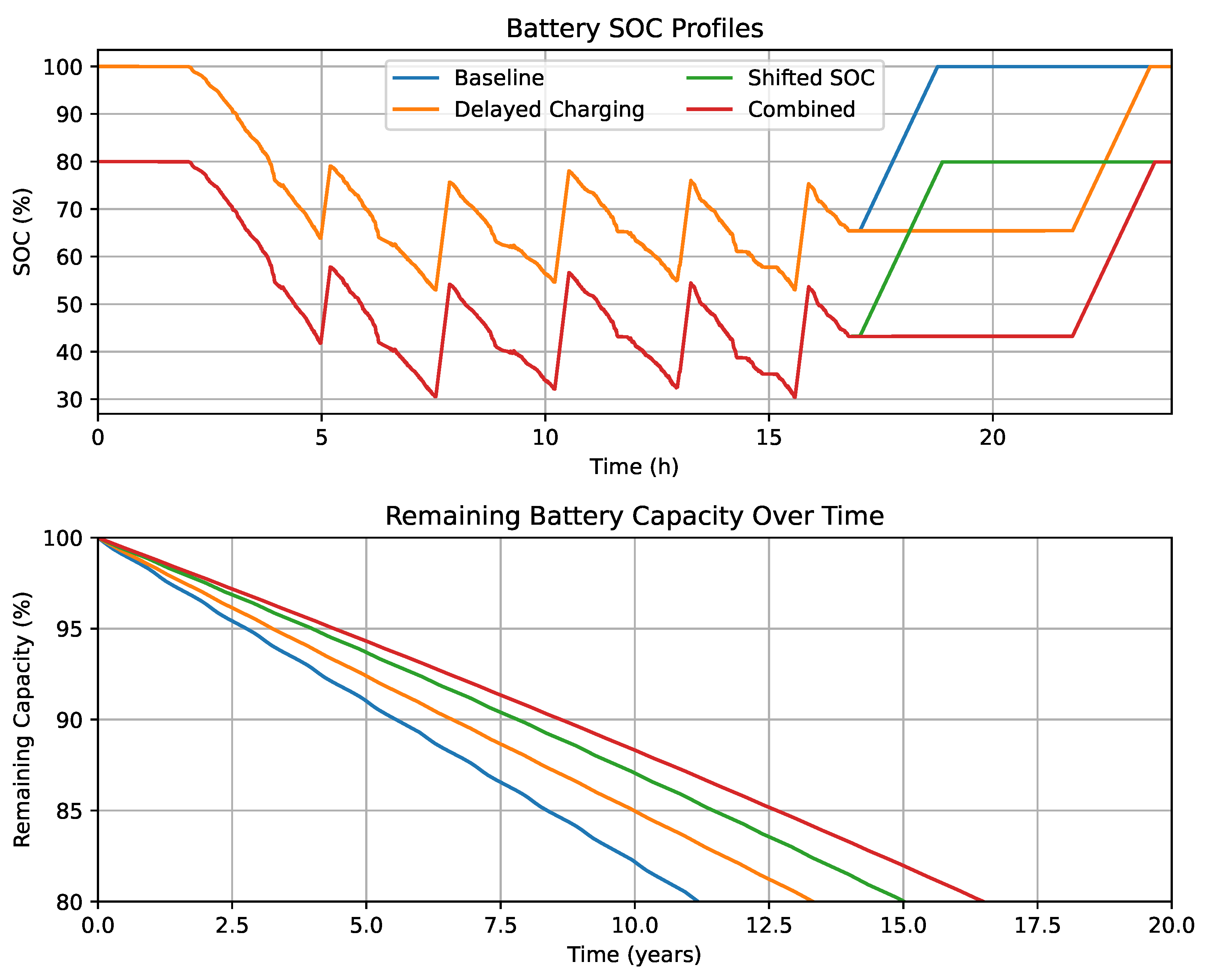
3.3. Estimation of the Impact of Operational Recommendations on Battery Lifetime

In the previous Section 3.2, the current battery operation strategy was analyzed, leading to two primary recommendations: (1) implement delayed depot charging and (2) reduce the state-of-charge (SOC) level during operation by 20%. Notably, these measures can be adopted without modifying the existing dispatch plan.

To quantify the potential extension of battery lifetime resulting from these recommendations, a battery aging model, as described in Ref. [40], is applied to a representative real-world drive cycle. This cycle is iteratively simulated until the end-of-life (EOL) threshold—defined as 80% remaining capacity—is reached. Subsequently, the drive cycle is modified to reflect each recommendation individually and in combination, and the corresponding EOL is determined for each scenario.

It is important to emphasize that this analysis serves as an illustrative example to demonstrate the potential benefits of operational strategy optimization. The results are based on a single repeated drive cycle and thus do not capture the full variability of real-world operations. The SOC profiles for the four drive cycle scenarios, along with the evolution of remaining battery capacity, are presented in Figure 8.

Based on the applied battery aging model, the current operational strategy results in a projected battery EOL after approximately 11 years of service. Implementing a delayed depot charging strategy extends the estimated battery lifetime to 13 years. A reduction in the operational SOC window increases the projected lifetime further to 15 years. When both strategies are applied in combination, the model predicts a maximum battery lifetime of approximately 16 years.

3.4. Environmental Impact

Based on the monitoring data, the reduction in CO₂-equivalent greenhouse gas emissions can be estimated when compared to diesel buses, where the emission of the German electricity mix in 2023 of 380 g/kWh is assumed [41]. The total energy consumption of the 12 m buses is 374.8 MWh for a total distance of 372.6 Tkm; the 18 m buses have traveled 3029.3 Tkm with 4766.2 MWh total energy consumption. Note that this value is calculated from the battery power during operation, thus charging losses are not yet accounted for. Assuming a charging energy efficiency of 95%, this results in the emission of approximately 2056.4 tons of CO₂ (12 m: 149.9 tons; 18 m: 1906.5 tons) and (indirect) emission factors of 402 g/km and 787 g/km for 12 m and 18 m electric buses, respectively. This can be compared to an equivalent fleet of diesel buses, where the real-world CO₂ emission factor of urban city buses are reported to be 871 g/km and 1416 g/km (average value for half load) for 12 m and 18 m, respectively [42,43]. Thus, an equivalent diesel bus fleet would have emitted about 4614.1 tons of CO₂ (12 m: 324.6 tons; 18 m: 4289.5 tons) or, in other words, about 2.2 times the amount of the electric bus fleet. On top, emissions of other gases like NO_x, CO, and THC, which are harmful to health and the environment, are prevented. With the corporate sustainability reporting directive (CSRD) of the European Union [44] obligating many companies to report their greenhouse gas emissions and present an emission reduction plan, long-term data monitoring allows for precise evaluations and tracking the emission reduction goals towards a greenhouse-gas-neutral fleet.

4. Discussion

This article presents various findings regarding energy consumption and battery operation for a fleet of solo buses and articulated BEBs. Instead of presenting a model approach to determining the energy consumption of BEBs, a large dataset was analyzed to determine the energy consumption with respect to the ambient temperature and average speed of the buses. The advantages are the straight-forward and easily understandable results as real-world data was used exclusively. The given values are to be understood as round-trip specific energy consumptions for urban bus drive cycles within average speed values between 20 and 28 km/h (12 m buses) and 18 and 24 km/h (18 m buses). By monitoring BEB fleets with different operational regimes, e.g., suburban/countryside drive cycles, the methodology could be applied, expanded, and further validated. The downside of the solely empirical approach is the requirement of long periods of data monitoring, and edge cases may not be properly represented. For instance, the elevation profile may influence the energy consumption between endpoints at the same height by up to 32.6% [45].

Furthermore, the operation of the bus fleet in terms of the battery SOC operating window, idle time conditions, and charging power was analyzed. For a battery-friendlier operation, the SOC window of operation should be shifted to lower values by about 20%. This is more severe for the solo buses which are often operated in the SOC range between 80% and 100%. Additionally, a smart depot charging system that charges the buses right before the next bus operation is recommended to reduce the vehicle idle time at high SOC levels and, thus, calendar aging. Based on a battery aging simulation with artificially modified drive cycles, implementing both recommendations may increase the battery lifetime from 11 years up to 16 years but may lead to bus delays of about 48 min per vehicle and year in the case of the articulated buses.

In order to safely reduce the operational SOC window, the 90th percentile curves can be used to estimate the energy demand of bus circulations and adjust the charging strategy according to ambient temperature and average speed of a bus circulation. The monitored bus fleet does not yet exhibit signs of advanced battery degradation, as no observable changes in energy efficiency, usable capacity, or operational SOC windows have occurred during the monitoring period. This finding aligns with expectations, given that all vehicles were essentially new at the beginning of this study, and the monitoring duration was limited to approximately 2.5 years. Nonetheless, as the fleet ages, gradual degradation—manifesting as reduced capacity and efficiency—can be expected. Once the battery capacity approaches critical thresholds (e.g., 80% of nominal capacity), it may become necessary to adjust the SOC window more conservatively to maintain operational reliability and prevent service disruptions. Therefore, future modeling efforts should incorporate appropriate battery aging models to account for long-term performance evolution and its implications for range, scheduling, and charging strategies [40,46].

The estimation of CO₂ emissions reveals that an equivalent diesel bus fleet would have emitted about 2.2 times the CO₂ of the electric buses assuming the 2023 electricity mix of Germany. Therefore, the emission of about 2560 tons of CO₂ was prevented corresponding to the total yearly CO₂ footprint of 452 EU citizens [47].

References

1. ACEA. New Commercial Vehicle Registrations: Vans +8.3%, Trucks −6.3%, Buses +9.2% in 2024. 2025. Available online: https://www.acea.auto/cv-registrations/new-commercial-vehicle-registrations-vans-8-3-trucks-6-3-buses-9-2-in-2024/ (accessed on 24 July 2025).
2. European Commission. Communication from the Commission to the European Parliament, the Counsil, the European Econimic and Social Committee and the Committee of the Regions; Technical Report COM/2020/562 Final; European Commission: Brussels, Belgium, 2020. [Google Scholar]
3. Grauers, A.; Borén, S.; Enerbäck, O. Total cost of ownership model and significant cost parameters for the design of electric bus systems. Energies 2020, 13, 3262. [Google Scholar] [CrossRef]
4. Kim, H.; Hartmann, N. Total Cost of Ownership Analysis of Battery Electric Buses for Public Transport System in a Small to Midsize City; International Association for Energy Economics: Cleveland, OH, USA, 2022. [Google Scholar]
5. Xiao, G.; Xiao, Y.; Shu, Y.; Ni, A.; Jiang, Z. Technical and economic analysis of battery electric buses with different charging rates. Transp. Res. Part Transp. Environ. 2024, 132, 104254. [Google Scholar] [CrossRef]
6. Jefferies, D.; Göhlich, D. A comprehensive TCO evaluation method for electric bus systems based on discrete-event simulation including bus scheduling and charging infrastructure optimisation. World Electr. Veh. J. 2020, 11, 56. [Google Scholar] [CrossRef]
7. Paul, T.; Yamada, H. Operation and charging scheduling of electric buses in a city bus route network. In Proceedings of the 17th International IEEE Conference on Intelligent Transportation Systems (ITSC), Qingdao, China, 8–11 October 2014; pp. 2780–2786. [Google Scholar] [CrossRef]
8. Xylia, M.; Leduc, S.; Patrizio, P.; Kraxner, F.; Silveira, S. Locating charging infrastructure for electric buses in Stockholm. Transp. Res. Part Emerg. Technol. 2017, 78, 183–200. [Google Scholar] [CrossRef]
9. Al-Ogaili, A.S.; Al-Shetwi, A.Q.; Al-Masri, H.M.; Babu, T.S.; Hoon, Y.; Alzaareer, K.; Babu, N.P. Review of the estimation methods of energy consumption for battery electric buses. Energies 2021, 14, 7578. [Google Scholar] [CrossRef]
10. Ji, J.; Bie, Y.; Zeng, Z.; Wang, L. Trip energy consumption estimation for electric buses. Commun. Transp. Res. 2022, 2, 100069. [Google Scholar] [CrossRef]
11. Gallet, M.; Massier, T.; Hamacher, T. Estimation of the energy demand of electric buses based on real-world data for large-scale public transport networks. Appl. Energy 2018, 230, 344–356. [Google Scholar] [CrossRef]
12. Abdelaty, H.; Mohamed, M. A prediction model for battery electric bus energy consumption in transit. Energies 2021, 14, 2824. [Google Scholar] [CrossRef]
13. Pihlatie, M.; Pippuri-Mäkeläinen, J. (Eds.) Electric Commercial Vehicles (ECV): Final Report; Number 348 in VTT Technology; VTT Technical Research Centre of Finland: Espoo, Finland, 2019. [Google Scholar] [CrossRef]
14. Fraunhofer IVI. Simulation Tool IVIsion. 2025. Available online: https://www.ivi.fraunhofer.de/en/research-fields/vehicle-and-propulsion-technologies/propulsion-technologies/simulation-tool-ivision.html (accessed on 4 July 2025).
15. Pamuła, T.; Pamuła, W. Estimation of the Energy Consumption of Battery Electric Buses for Public Transport Networks Using Real-World Data and Deep Learning. Energies 2020, 13, 2340. [Google Scholar] [CrossRef]
16. Xing, Y.; Li, Y.; Liu, W.; Li, W.; Meng, L. Operation Energy Consumption Estimation Method of Electric Bus Based on CNN Time Series Prediction. Math. Probl. Eng. 2022, 2022, 6904387. [Google Scholar] [CrossRef]
17. Jalkanen, K.; Karppinen, J.; Skogström, L.; Laurila, T.; Nisula, M.; Vuorilehto, K. Cycle aging of commercial NMC/graphite pouch cells at different temperatures. Appl. Energy 2015, 154, 160–172. [Google Scholar] [CrossRef]
18. Plattard, T.; Barnel, N.; Assaud, L.; Franger, S.; Duffault, J.M. Combining a Fatigue Model and an Incremental Capacity Analysis on a Commercial NMC/Graphite Cell under Constant Current Cycling with and without Calendar Aging. Batteries 2019, 5, 36. [Google Scholar] [CrossRef]
19. Han, X.; Lu, L.; Zheng, Y.; Feng, X.; Li, Z.; Li, J.; Ouyang, M. A review on the key issues of the lithium ion battery degradation among the whole life cycle. eTransportation 2019, 1, 100005. [Google Scholar] [CrossRef]
20. Edge, J.S.; O’Kane, S.; Prosser, R.; Kirkaldy, N.D.; Patel, A.N.; Hales, A.; Ghosh, A.; Ai, W.; Chen, J.; Yang, J.; et al. Lithium ion battery degradation: What you need to know. Phys. Chem. Chem. Phys. 2021, 23, 8200–8221. [Google Scholar] [CrossRef] [PubMed]
21. Xu, B.; Oudalov, A.; Ulbig, A.; Andersson, G.; Kirschen, D.S. Modeling of lithium-ion battery degradation for cell life assessment. IEEE Trans. Smart Grid 2016, 9, 1131–1140. [Google Scholar] [CrossRef]
22. Ecker, M.; Gerschler, J.B.; Vogel, J.; Käbitz, S.; Hust, F.; Dechent, P.; Sauer, D.U. Development of a lifetime prediction model for lithium-ion batteries based on extended accelerated aging test data. J. Power Sources 2012, 215, 248–257. [Google Scholar] [CrossRef]
23. Rumberg, B.; Schwarzkopf, K.; Epding, B.; Stradtmann, I.; Kwade, A. Understanding the different aging trends of usable capacity and mobile Li capacity in Li-ion cells. J. Energy Storage 2019, 22, 336–344. [Google Scholar] [CrossRef]
24. Rumberg, B.; Epding, B.; Stradtmann, I.; Schleder, M.; Kwade, A. Holistic calendar aging model parametrization concept for lifetime prediction of graphite/NMC lithium-ion cells. J. Energy Storage 2020, 30, 101510. [Google Scholar] [CrossRef]
25. Keil, P.; Schuster, S.F.; Wilhelm, J.; Travi, J.; Hauser, A.; Karl, R.C.; Jossen, A. Calendar aging of lithium-ion batteries. J. Electrochem. Soc. 2016, 163, A1872. [Google Scholar] [CrossRef]
26. Baghdadi, I.; Briat, O.; Delétage, J.Y.; Gyan, P.; Vinassa, J.M. Lithium battery aging model based on Dakin’s degradation approach. J. Power Sources 2016, 325, 273–285. [Google Scholar] [CrossRef]
27. Torregrosa, A.J.; Broatch, A.; Olmeda, P.; Agizza, L. A semi-empirical model of the calendar ageing of lithium-ion batteries aimed at automotive and deep-space applications. J. Energy Storage 2024, 80, 110388. [Google Scholar] [CrossRef]
28. Gao, Y.; Jiang, J.; Zhang, C.; Zhang, W.; Jiang, Y. Aging mechanisms under different state-of-charge ranges and the multi-indicators system of state-of-health for lithium-ion battery with Li (NiMnCo) O2 cathode. J. Power Sources 2018, 400, 641–651. [Google Scholar] [CrossRef]
29. Preger, Y.; Barkholtz, H.M.; Fresquez, A.; Campbell, D.L.; Juba, B.W.; Romàn-Kustas, J.; Ferreira, S.R.; Chalamala, B. Degradation of commercial lithium-ion cells as a function of chemistry and cycling conditions. J. Electrochem. Soc. 2020, 167, 120532. [Google Scholar] [CrossRef]
30. de Hoog, J.; Timmermans, J.M.; Ioan-Stroe, D.; Swierczynski, M.; Jaguemont, J.; Goutam, S.; Omar, N.; Van Mierlo, J.; Van Den Bossche, P. Combined cycling and calendar capacity fade modeling of a Nickel-Manganese-Cobalt Oxide Cell with real-life profile validation. Appl. Energy 2017, 200, 47–61. [Google Scholar] [CrossRef]
31. Gao, Z.; Xie, H.; Yang, X.; Niu, W.; Li, S.; Chen, S. The Dilemma of C-Rate and Cycle Life for Lithium-Ion Batteries under Low Temperature Fast Charging. Batteries 2022, 8, 234. [Google Scholar] [CrossRef]
32. Kim, D.H.; Lee, J.; Shin, K.; Kim, K.B.; Chung, K.Y. Empirical Capacity Degradation Model for a Lithium-Ion Battery Based on Various C-Rate Charging Conditions. J. Electrochem. Sci. Technol. 2024, 15, 414–420. [Google Scholar] [CrossRef]
33. Schreiber, M.; Gamra, K.A.; Bilfinger, P.; Teichert, O.; Schneider, J.; Kröger, T.; Wassiliadis, N.; Ank, M.; Rogge, M.; Schöberl, J.; et al. Understanding lithium-ion battery degradation in vehicle applications: Insights from realistic and accelerated aging tests using Volkswagen ID.3 pouch cells. J. Energy Storage 2025, 112, 115357. [Google Scholar] [CrossRef]
34. Vermeer, W.; Chandra Mouli, G.R.; Bauer, P. A Comprehensive Review on the Characteristics and Modeling of Lithium-Ion Battery Aging. IEEE Trans. Transp. Electrif. 2022, 8, 2205–2232. [Google Scholar] [CrossRef]
35. Leijon, J. Charging strategies and battery ageing for electric vehicles: A review. Energy Strategy Rev. 2025, 57, 101641. [Google Scholar] [CrossRef]
36. Fraunhofer IVI. Remote Battery Diagnosis. 2025. Available online: https://www.ivi.fraunhofer.de/en/research-fields/electromobility/remote-battery-diagnosis.html (accessed on 4 July 2025).
37. Zippenfenig, P. Open-Meteo.com Weather API; Zenodo: Geneva, Switzerland, 2023. [Google Scholar] [CrossRef]
38. Weiss, M.; Cloos, K.C.; Helmers, E. Energy efficiency trade-offs in small to large electric vehicles. Environ. Sci. Eur. 2020, 32, 46. [Google Scholar] [CrossRef]
39. Al-Wreikat, Y.; Serrano, C.; Sodré, J.R. Driving behaviour and trip condition effects on the energy consumption of an electric vehicle under real-world driving. Appl. Energy 2021, 297, 117096. [Google Scholar] [CrossRef]
40. Lehmann, T.; Berendes, E.; Kratzing, R.; Sethia, G. Learning the Ageing Behaviour of Lithium-Ion Batteries Using Electric Vehicle Fleet Analysis. Batteries 2024, 10, 432. [Google Scholar] [CrossRef]
41. Icha, P.; Lauf, D.T. Entwicklung der Spezifischen Treibhausgas-Emissionen des Deutschen Strommix in den Jahren 1990–2023; Technical Report CLIMATE CHANGE 23/2024; Umweltbundesamt: Dessau-Roßlau, Germany, 2024; ISSN 1862-4359. [Google Scholar]
42. Özener, O.; Özkan, M. Fuel consumption and emission evaluation of a rapid bus transport system at different operating conditions. Fuel 2020, 265, 117016. [Google Scholar] [CrossRef]
43. Zhang, S.; Wu, Y.; Liu, H.; Huang, R.; Yang, L.; Li, Z.; Fu, L.; Hao, J. Real-world fuel consumption and CO2 emissions of urban public buses in Beijing. Appl. Energy 2014, 113, 1645–1655. [Google Scholar] [CrossRef]
44. European Parliament and Council of the European Union. Directive (EU) 2022/2464 of the European Parliament and of the Council of 14 December 2022 amending Regulation (EU) No 537/2014, Directive 2004/109/EC, Directive 2006/43/EC and Directive 2013/34/EU, as regards corporate sustainability reporting. Off. J. Eur. Union 2022, L322, 15–80. [Google Scholar]
45. Liu, J.; Feng, L.; Li, Z. The Optimal Road Grade Design for Minimizing Ground Vehicle Energy Consumption. Energies 2017, 10, 700. [Google Scholar] [CrossRef]
46. Lehmann, T.; Weiß, F. Lithium-Ion Battery Aging Analysis of an Electric Vehicle Fleet Using a Tailored Neural Network Structure. Appl. Sci. 2023, 13, 4448. [Google Scholar] [CrossRef]
47. EDGAR (Emissions Database for Global Atmospheric Research). GHG Emissions of All World Countries: 2024 Report; Joint Research Centre, Publications Office of the European Union: Luxembourg, 2024; Available online: https://edgar.jrc.ec.europa.eu/report_2024 (accessed on 4 July 2025).
Figure 1. Scheme of the most important factors influencing the SEC. The light green factors are directly addressed in the energy consumption analysis. Dark green factors are indirectly addressed by the daily grouping and blue factors are neglected so far.
Wevj 16 00419 g001
Figure 2. (a) Speed signal of an example operating day with identified trips marked by the green and red dashed lines. (b) Vehicle speed timeseries of an identified trip (see markings). (cg) Various signals within the time span of the example trip (see y-axis labels). Note that in (e), negative values of the battery power indicate power drawn from the battery; positive values charge the battery.
Wevj 16 00419 g002
Figure 3. Histograms of the daily grouped dataset. Panels (ac) presents the number of operating days of the solo buses vs. distance-weighted average temperature, average speed, and distance-weighted average vehicle weight, respectively. Panels (df) show the same histograms for the articulated buses.
Wevj 16 00419 g003
Figure 4. Battery energy consumption in kWh/km vs. ambient temperature at different average speed ranges. (a) Mean energy consumption for solo buses and (b) articulated buses with the 10th and 90th percentile given by the shaded area. (c) Separate plots for the 90th percentile of the energy consumption for solo and (d) articulated buses as a useful quantity for disposition planning. Note that below 4 °C an additional oil heater is used to heat the bus interior to reduce battery energy consumption.
Wevj 16 00419 g004
Figure 5. Driven kilometers of solo buses in the given SOC range for (a) the entire monitoring period, (b) summer months (June, July, and August), and (c) winter months (December, January, and February), panels (df) show the evaluations for the articulated buses. Colors in the bar chart distinguish individual buses. Due to the higher energy consumption, the average SOC of the articulated buses is roughly 6% lower in winter than in summer. However, regarding the rules for increasing battery lifetime, the operating window should be shifted to a lower SOC.
Wevj 16 00419 g005
Figure 6. Vehicle idle time (vehicle at rest and no charging process detected) at given SOC level for (a) solo buses and (b) articulated buses. Colors in the bar chart distinguish individual buses.
Wevj 16 00419 g006
Figure 7. Charged energy at different charging power for (a) solo buses and (b) articulated buses throughout the year 2024. Charging power below 100 kW typically indicates depot charging, whereas higher charging power is used at opportunity chargers. Colors in the bar chart distinguish individual buses.
Wevj 16 00419 g007
Figure 8. SOC profiles of four drive cycle scenarios (baseline, delayed depot charging, reduced SOC window, and combined strategy) for a day of operation. The lower plot shows the remaining battery capacity as a function of years in operation illustrating the impact of each operational strategy on battery aging.
Wevj 16 00419 g008