Research on Multi-Target Point Path Planning Based on APF and Improved Bidirectional RRT* Fusion Algorithm

Abstract

In order to solve the problems of traditional RRT algorithms that are too random in planning, have low planning efficiency, and have insufficient security, this paper proposes an algorithm that fuses APF and the improved bidirectional RRT* algorithm and proposes a heuristic planning strategy to sort multiple target points so that the fusion improvement algorithm can traverse multiple target points with a short path length. This study also aims to improve the RRT* algorithm by using optimization strategies such as bidirectional sampling and adding an adaptive target bias strategy to improve its efficiency in obtaining global paths. The obstacle expansion strategy is used in the APF algorithm to expand the repulsion effect, and the APF algorithm after the obstacle expansion is fused with the improved bidirectional RRT* algorithm, adding gravitational potential field-guided sampling at random points, avoiding local optimum solution, and improving the sampling efficiency while accelerating the acquisition of global paths. The redundant node deletion strategy is introduced to simplify the path, and the repulsive potential field is used to improve the Bezier smoothing method, avoiding collisions caused by path distortion due to smoothing. A multi-target point heuristic planning strategy is proposed to achieve shorter global paths while maintaining shorter local paths, taking into account both local solutions and optimal solutions, so that the fusion algorithm can be applied to the path planning of multi-target points.

1. Introduction

With the rapid development of intelligent driving technology and the increasing demand for intelligence in the field of transportation, the link between the two is becoming closer and closer, and the intelligent transportation mode is constantly developing; this not only improves transportation efficiency but also shows great potential in reducing energy consumption and optimizing the allocation of resources [1].

Path planning is one of the key technologies associated with intelligent driving technology in automobiles, and it has long been a major hot topic in research on intelligent driving cars at home and abroad. The essence of path planning is to calculate an optimal path from the starting position to the target position based on the current environment information through a planning algorithm. This path is finally sent to the control layer to guide the vehicle to the target position. For the planning of global paths, the commonly used algorithms currently include graph search-based algorithms represented by the A* algorithm, sampling-based algorithms represented by RRT-type algorithms, and intelligent algorithms. Among them, RRT algorithms are mostly used to solve problems with larger and more complex maps.

The RRT algorithm, also known as the Rapid-exploration Random Tree (RRT), is an incremental algorithm based on random sampling. It was proposed by LaValle et al. [2]. This algorithm can maintain its search efficiency in high-latitude space. Compared with the same sampling-based PRM algorithm [3] (Probabilistic Roadmap Method), the RRT algorithm is faster. Based on the RRT algorithm, Karaman et al. proposed the RRT* algorithm in 2011 [4] and added parent node reselection and node reconnection strategies based on the RRT algorithm, which improved the quality of path planning, but its convergence speed was still slow. Ganesan et al. [5] added a hybrid sampling strategy based on the traditional RRT* algorithm, that is, combining non-uniform sampling and uniform sampling to enhance the convergence speed of the algorithm, balancing the characteristics of limited exploration and the exhaustive exploration of traditional RRT* algorithms, overall improving the speed of path planning and achieving good results in complex and narrow environments. JinGu et al. [6] proposed an RRT-Connect algorithm based on triangular inequality, connecting child nodes and their parent nodes to form a triangle and re-wiring the triangle inequality on the basis of collision-free, making the result closer to the optimal solution. Compared with the basic RRT-Connect algorithm, the resulting path length is shortened, but some nodes may make the path not smooth enough after being optimized by the algorithm. LiY et al. [7] proposed PQ-RRT* in combination with the advantages of P-RRT* and Quick-RRT*. This algorithm combines the potential function change sampling strategy, the parent node search range, and node reconnection in Quick-RRT* and comprehensively improves it and finally can quickly converge to get the optimal solution, but the algorithm does not take into account the kinematic constraints of the actual carrier and may perform poorly in complex situations. Faroni et al. [8] defined a hybrid sampler to reasonably select informed sampling or local sampling to improve RRT* algorithms such as Informed-RRT* and improve the convergence speed of the algorithm. In summary, the current algorithm improvements for RRT type mainly focus on improving sampling efficiency, reducing the number of nodes, solving multifold problems, and making the planned path smoother.

Although, for the RRT class algorithm, aforementioned scholars have made more improvements or algorithm fusion, most of the algorithm considerations are still not comprehensive enough for the RRT class algorithm applied to multiple target location planning research to improve the consideration of less, and the resulting path is difficult to take into account the iterative length, path length, the ability to avoid obstacles, and to meet the needs of vehicle kinematics. In this paper, a bi-directional improved RRT* algorithm incorporating the improved APF algorithm is proposed and applied to solve the multi-target point path planning problem. The RRT* algorithm is improved by using bi-directional sampling and proposing an adaptive target bias strategy to speed up the path acquisition. A redundant node deletion strategy is added to path simplification of the resulting paths. The APF algorithm is improved by obstacle inflation and fuses the improved RRT* and improved APF algorithms. An improved Bezier smoothing method with potential field auxiliary point insertion is proposed for path smoothing processing to reduce obstacle collisions due to path distortion situations during smoothing. A heuristic planning strategy is proposed so that the fused improved algorithm can be applied to solve multiple target point problems. Through the above fusion and improvement, the algorithm is able to solve multiple target point problems while taking into account time, length, obstacle avoidance capability, and path smoothing.

2. Traditional Algorithm

2.1. RRT* Algorithm

The core of the RRT algorithm is to perform random sampling within the global feasible range, find the nearest node in the search tree as the next reference node under the premise of collision, and continue to grow at a given growth step until the maximum growth limit is reached or a feasible path is realized. But in fact, since the RRT algorithm constantly diverges sampling on the tree of the same backbone, it can only ensure that the searched path is a “feasible solution” and not necessarily an “optimal solution”. Moreover, due to random sampling, the resulting path may have many vertices, which is not conducive to the actual state of vehicle driving; in complex environments, search efficiency may be reduced due to obstacle limitations or narrow search channels.

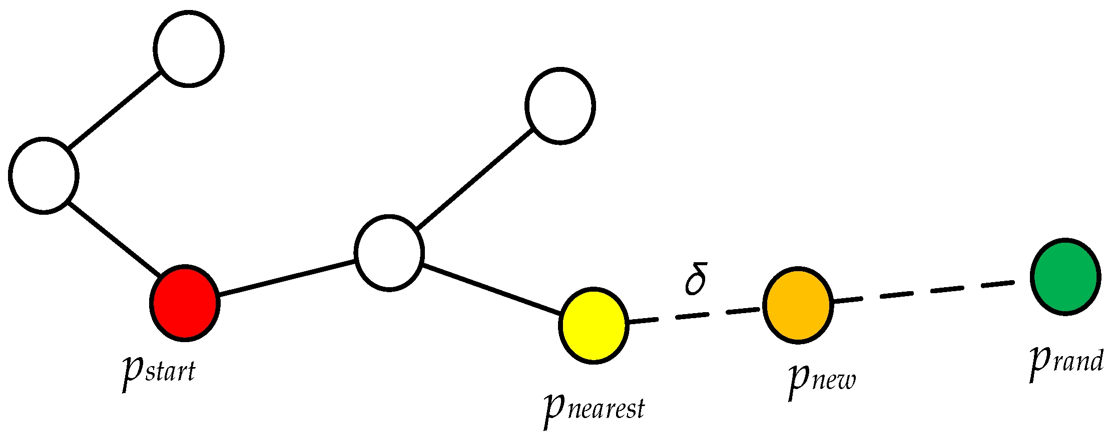
In the ordinary RRT algorithm, the initial position is the starting node $p_{start}$ of the entire random tree, and then a random point is generated in the environment, which is named random point $p_{rand}$. The closest node $p_{nearest}$ is found within a certain range, and the two nodes are connected and collision detection is performed. If the connection line does not collide with an obstacle, a distance of step $\delta$ will be grown from the closest node $p_{nearest}$ to the random node $p_{rand}$ in the direction of the connection line. If the growing node does not collide with the obstacle, the node at that location is the newly generated node $p_{start}$, which is added to the extension tree, but if a collision is found during detection, delete this node. The above process continues to repeat in the algorithm until the target node $p_{goal}$ is added to the extension tree or the iteration reaches the maximum number of times; the algorithm stops. 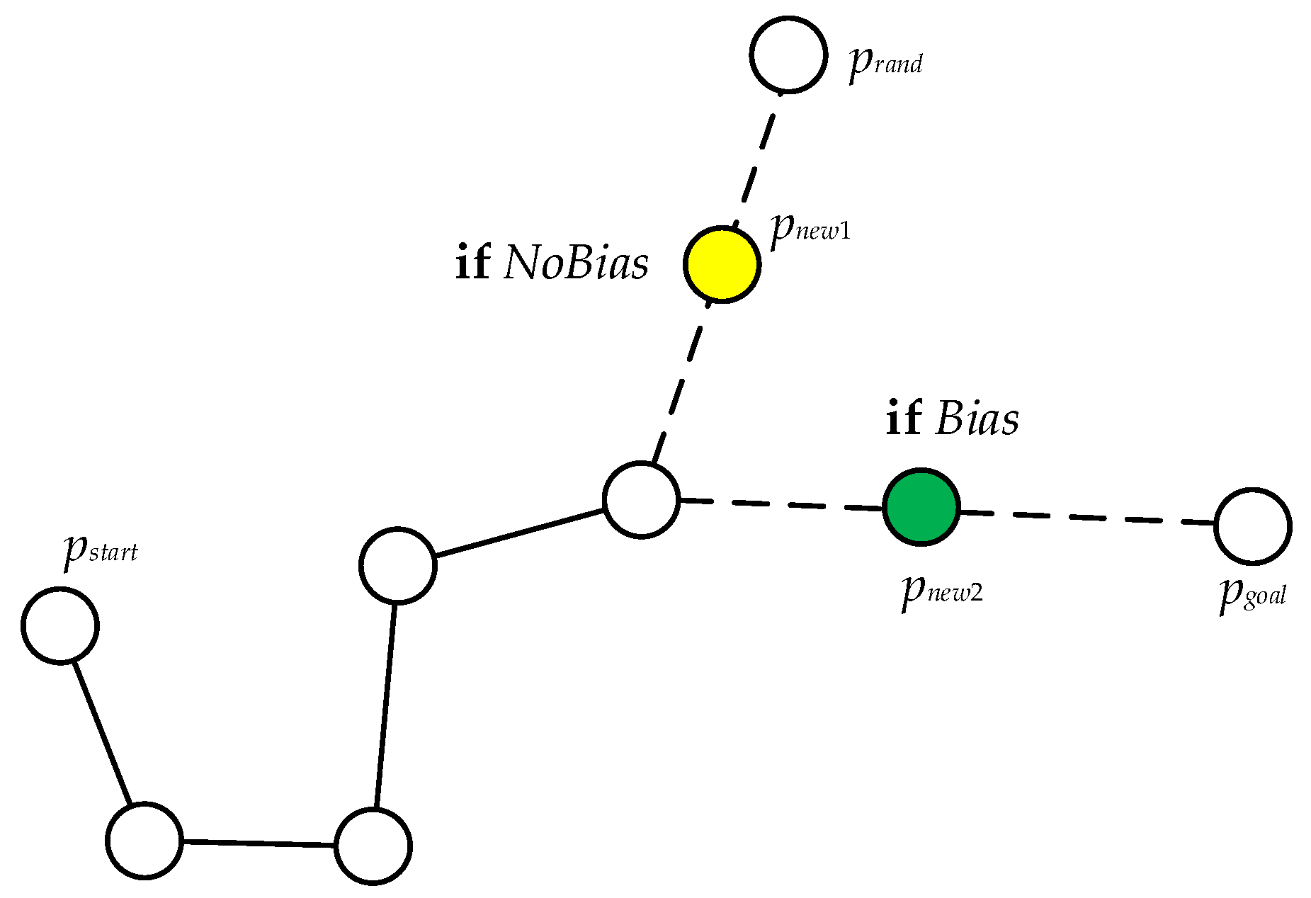At this time, you can trace back to the entire expansion tree from the connection line from the starting node $p_{start}$ o the target node $p_{goal}$ and each node to obtain a global path. The way of generating new nodes in the random tree is shown in Figure 1, where the red point is the starting node $p_{start}$, the green node is the generated random point $p_{rand}$, and the orange node $p_{new}$ is a new node obtained by growing a step toward the random point at the nearest node $p_{nearest}$ from $p_{rand}$ [9].

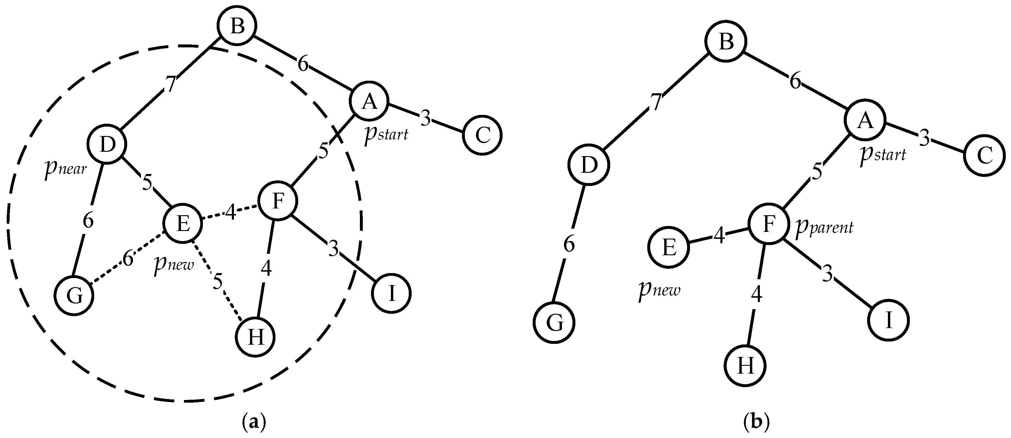
Based on the above RRT algorithm, the RRT* algorithm introduces parent node reselect and node reconnection strategies [10]. Among them, parent node reselection refers to searching for a node with a smaller cost than its parent node in the circle where the new node $p_{new}$ is the center of the circle and using this node as a new parent node $p_{parent}$ instead of the original parent node $p_{near}$ of the new node. The parent node reselect strategy as shown in Figure 2.

In

Table 1. Expand tree reselects parent node cost.

Possible Parent Node	New Path	Total Cost
F	A-F-E	5 + 4 = 9
G	A-B-D-G-E	6 + 7 + 6 + 6 = 25
H	A-F-H-E	5 + 4 + 5 = 14

, the node is a new node. In addition to its own parent node $D$, there are three possible parent nodes. The total cost of these three nodes is compared with the total cost of the path of the parent node. The parent node on the path with the smallest cost is taken. Here, the total cost of the $F$ and $H$ nodes is less than the total cost of the original parent node, but obviously the total cost of the node is smaller, so the $F$ node becomes the new parent node $p_{parent}$ of the $E$ node. This process significantly reduces the total path length of the random tree. The pseudocode for this strategy is shown in Algorithm 1.

Algorithm 1. Parent Node Reselect Strategy
1:	$p_{min}\leftarrow p_{nearest}$
2:	$min\_cost\leftarrow \mathrm{p}\mathrm{a}\mathrm{t}\mathrm{h}\_\mathrm{c}\mathrm{o}\mathrm{s}\mathrm{t}\left(p_{nearest}\right)+\mathrm{D}\mathrm{i}\mathrm{s}\mathrm{t}\mathrm{a}\mathrm{n}\mathrm{c}\mathrm{e}(p_{nearest},p_{new})$
3:	for each $p_{near}\in X_{near}$ do
4:	$dis\_cost\leftarrow \mathrm{p}\mathrm{a}\mathrm{t}\mathrm{h}\_\mathrm{c}\mathrm{o}\mathrm{s}\mathrm{t}\left(p_{near}\right)++\mathrm{D}\mathrm{i}\mathrm{s}\mathrm{t}\mathrm{a}\mathrm{n}\mathrm{c}\mathrm{e}(p_{near},p_{new})$
5:	if $\mathrm{C}\mathrm{o}\mathrm{l}\mathrm{l}\mathrm{i}\mathrm{s}\mathrm{i}\mathrm{o}\mathrm{n}\mathrm{C}\mathrm{h}\mathrm{e}\mathrm{c}\mathrm{k}(p_{near},p_{new},Obs)$ then
6:	if $dis\_cost<min\_cost$
7:	$min\_cost\leftarrow dis\_cost$
8:	$p_{min}\leftarrow p_{near}$
9:	end if
10:	end if
11:	end for
12:	return $p_{min}$

The node reconnection strategy refers to finding all nearby nodes within a certain range of the new node $p_{new}$ after reselecting the parent node and using the new node $p_{new}$ as the parent node to calculate the generation value of its arrival at other nearby nodes. If the cost is less than the price of the nearby node reaching its original parent node, then $p_{new}$ will become the new parent node of this node. The node reconnection strategy as shown in Figure 3.

It can be seen in

Table 2. Path cost after node reconnection strategy.

Near Node	Original Path Cost	New Path	New Path Cost
D	6 + 7 = 13	A-F-E-D	5 + 4 + 5 = 14
G	6 + 7+6 = 19	A-F-E-G	5 + 4 + 6 = 15
H	5 + 4 = 9	A-F-E-H	5 + 4 + 5 = 14

that the $E$ node is the parent node, and its adjacent nodes are $D$, $G$, and $H$, respectively. The total cost of calculating the original path of these three nodes is compared with the total cost of the path of node $E$ as the parent node. The total cost of the $G$ node is less than the total cost of the original parent node. Therefore, the $E$ node becomes the new parent node of the $G$ node, and this process also reduces the total path length of the random tree. The pseudocode of the node reconnection strategy is shown in Algorithm 2.

Algorithm 2. Node Reconnection Strategy
1:	$G=(V,E)$
2:	for each $p_{near}\in X_{near}$do
3:	if $CollisionCheck(p_{near},p_{new},Obs)\leftarrow False$ and $distance\left(p_{near},p_{new}\right)+$
	$min\_cost\left(p_{new}\right)<min\_cost\left(p_{near}\right)$ then
4:	$p_{parent}\leftarrow p_{new}$
5:	$E\leftarrow \mathrm{R}\mathrm{e}\mathrm{c}\mathrm{o}\mathrm{n}\mathrm{n}\mathrm{e}\mathrm{c}\mathrm{t}(p_{near},p_{new})$
6:	end if
7:	$\mathbf{e}\mathbf{n}\mathbf{d} \mathbf{f}\mathbf{o}\mathbf{r}$
8:	return  $G=(V,E)$

Overall, the RRT* algorithm reduces the overall length of the path by introducing two strategies and optimizes the path quality.

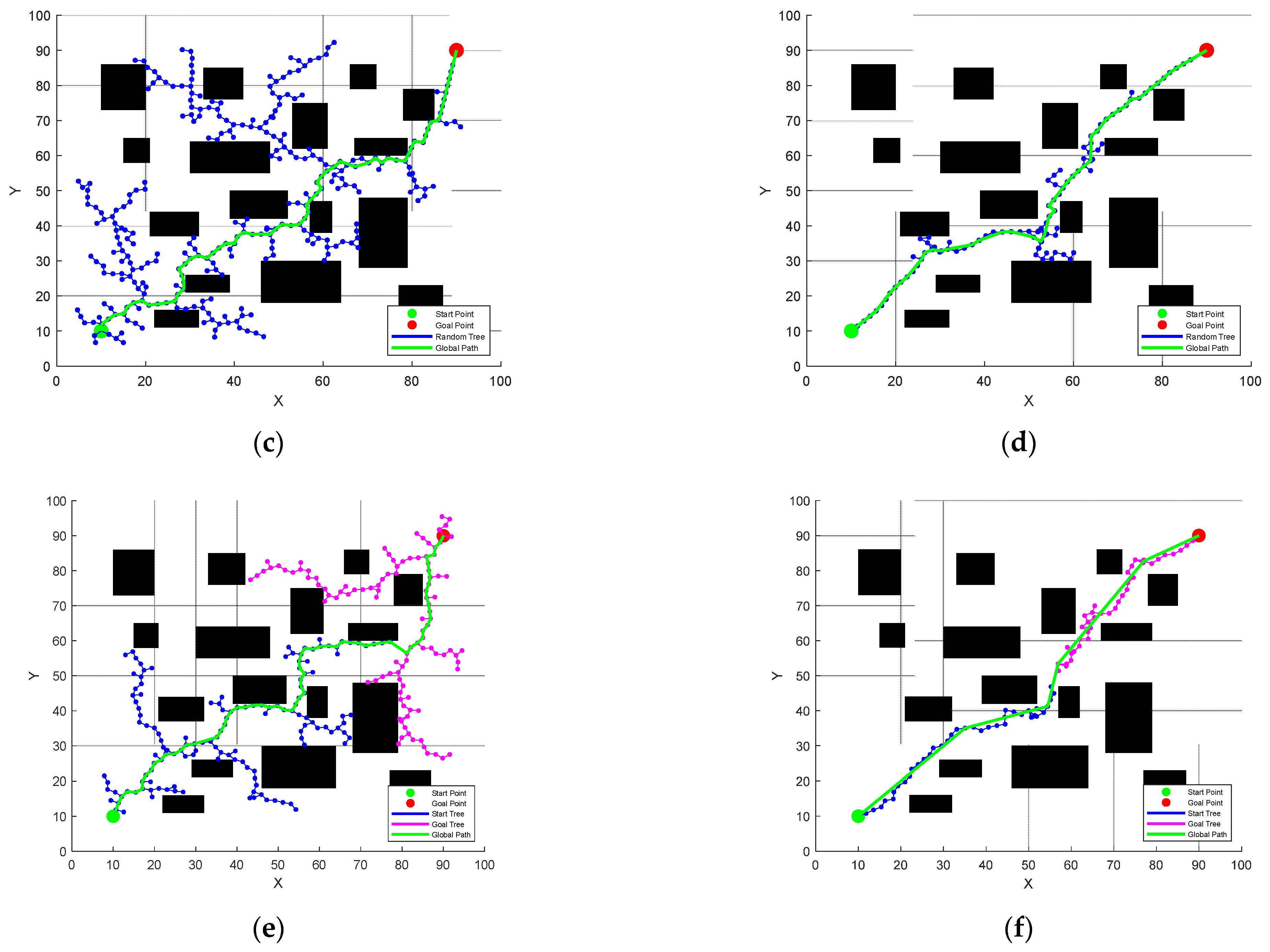
2.2. Bi-RRT* Algorithm

The Bi-RRT* algorithm (Bi-directional RRT*) is improved on the basis of the RRT* algorithm [11]. Compared with the RRT* algorithm, the Bi-RRT* algorithm uses the initial position and target position in the global area as the starting points of two random trees, namely $p_{start1}$ and $p_{start2}$. Then, starting with two starting points, the RRT* process is performed separately, and two expansion trees, $T_1$ and $T_2$, are gradually generated. During the operation, the parent node reselect strategy and node reconnection strategy of the RRT* algorithm are also performed, and the path is expanded and optimized at the same time. The condition for the operation to terminate is to reach the maximum number of iterations $N$ or make the distance between nodes $p_{T1}$ in $T_1$ and node $p_{T2}$ in $T_2$ not greater than the node growth step $\delta$ set in the Bi-RRT* algorithm. At this time, the two nodes, $p_{T1}$ and $p_{T2}$, will be connected; that is, the two expansion trees are merged into an expansion tree, and a global path from $p_{start1}$ to $p_{start2}$ is traced back. Its pseudocode is shown in Algorithm 3.

Algorithm 3. Bi-RRT* algorithm
1:	Initialize trees $T_1\leftarrow \left\{p_{start1}\right\}$,$T_2\leftarrow \left\{p_{start2}\right\}$
2:	for $i=1$ to $N$ do
3:	$p_{rand}\leftarrow \mathrm{R}\mathrm{a}\mathrm{n}\mathrm{d}\mathrm{o}\mathrm{m}\mathrm{S}\mathrm{a}\mathrm{m}\mathrm{p}\mathrm{l}\mathrm{e}\left(\right)$
4:	$p_{new1}\leftarrow \mathrm{E}\mathrm{x}\mathrm{t}\mathrm{e}\mathrm{n}\mathrm{d}\mathrm{t}\mathrm{r}\mathrm{e}\mathrm{e}\left(T_1,p_{rand},\delta ,Obs\right)$
5:	$T_1\leftarrow \mathrm{N}\mathrm{o}\mathrm{d}\mathrm{e}\mathrm{R}\mathrm{e}\mathrm{c}\mathrm{o}\mathrm{n}\mathrm{n}\mathrm{e}\mathrm{c}\mathrm{t}\mathrm{i}\mathrm{o}\mathrm{n}\left(T_1,p_{new1},\delta ,Obs\right)$
6:	$p_{new2}\leftarrow \mathrm{E}\mathrm{x}\mathrm{t}\mathrm{e}\mathrm{n}\mathrm{d}\mathrm{t}\mathrm{r}\mathrm{e}\mathrm{e}\left(T_2,p_{rand},\delta ,Obs\right)$
7:	$T_2\leftarrow \mathrm{N}\mathrm{o}\mathrm{d}\mathrm{e}\mathrm{R}\mathrm{e}\mathrm{c}\mathrm{o}\mathrm{n}\mathrm{n}\mathrm{e}\mathrm{c}\mathrm{t}\mathrm{i}\mathrm{o}\mathrm{n}\left(T_2,p_{new2},\delta ,Obs\right)$
8:	if $\mathrm{D}\mathrm{i}\mathrm{s}\mathrm{t}\mathrm{a}\mathrm{n}\mathrm{c}\mathrm{e}(p_{T1},p_{T2})\le \delta$ then
9:	$Path\leftarrow \mathrm{B}\mathrm{a}\mathrm{c}\mathrm{k}\mathrm{t}\mathrm{r}\mathrm{a}\mathrm{c}\mathrm{k}\mathrm{P}\mathrm{a}\mathrm{t}\mathrm{h}\left(T_1,T_2,p_{T1},p_{T2}\right)$
10:	end if
11:	end for
12:	return  $Path$

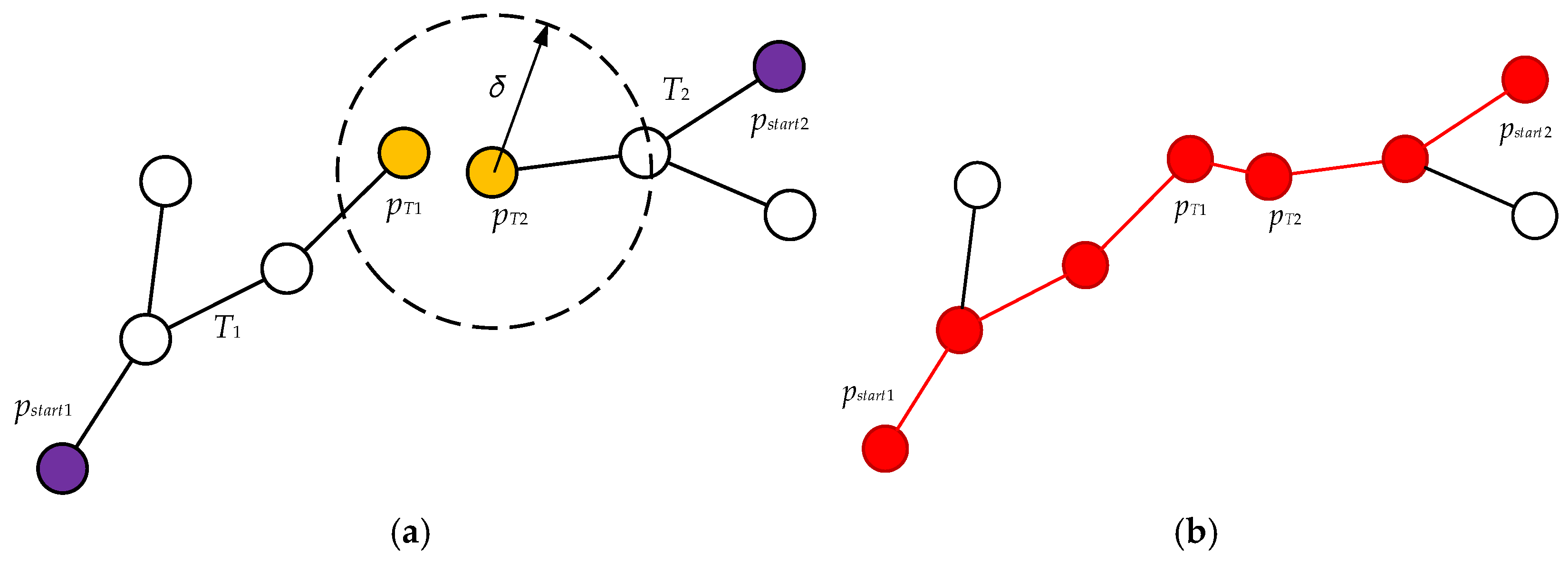
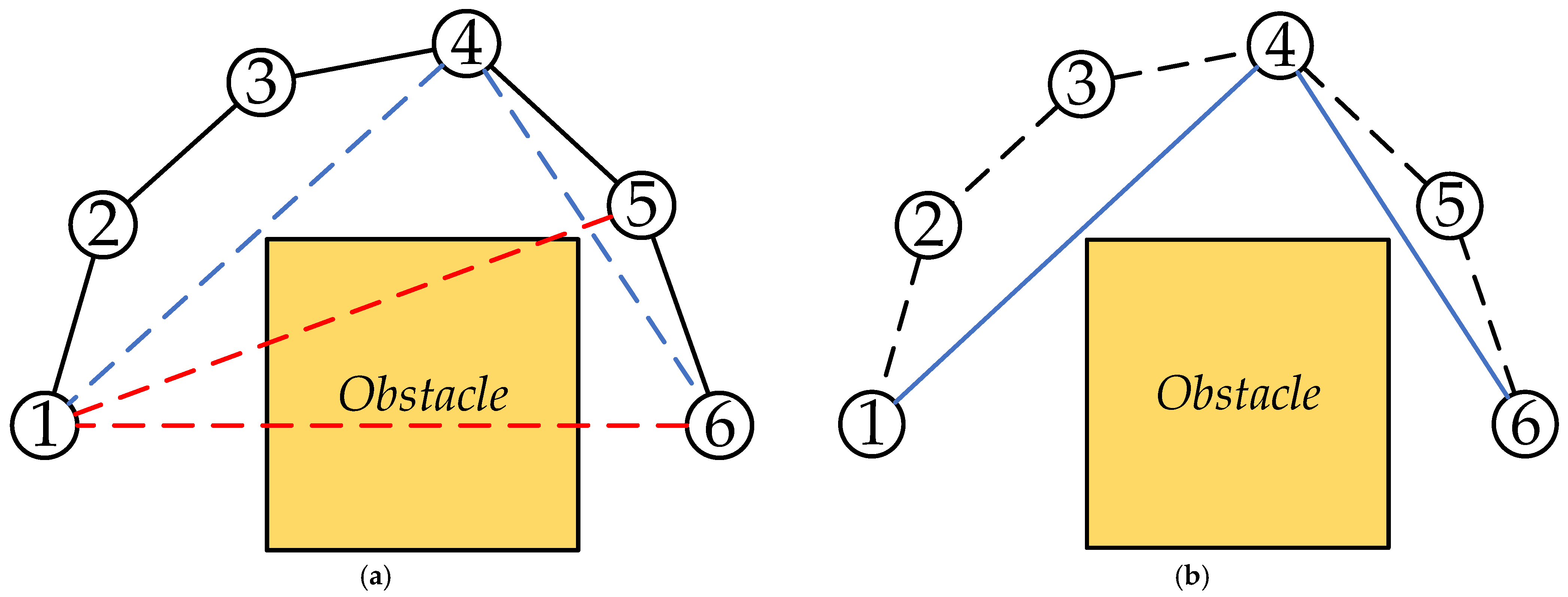
For Figure 4, the left is the random tree $T_1$ grown from the starting point $p_{start1}$, and the right is the random tree $T_2$ grown from the global end point $p_{start2}$, and $p_{T1}$ and $p_{T2}$ are points in the two random trees respectively. At this time, the point among these two points is the center and the growth step $\delta$ is the radius as a circular determination range. It can be seen that $p_{T1}$ is already within the selection range of $p_{T2}$, so the two points are connected and a complete global path is traced back. The red line in the Figure 4b is the global path.

Since the growth of the random tree grows opposite to the starting point and the target point, and the parent node reselecting and node reconnection strategies in the original RRT* algorithm are retained, the Bi-RRT* algorithm improves the search efficiency and makes the path better.

2.3. APF Algorithm

APF algorithm (Artificial Potential Field algorithm), which implements path planning by simulating a virtual potential field environment in the map. When planning the vehicle’s path, use the current position of the vehicle as the starting point of the global path and the target position as the target point, and apply a potential field on the target point and the obstacles in the map so that the target point has a gravitational effect on the vehicle and the obstacles have a repulsive effect on the vehicle. Under the combined force, guide the vehicle to plan and avoid obstacles [12].

In the potential field, assuming the gravitational potential field is $U_{att}\left(d\right)$, the gravitational force on the vehicle is $F_{att}\left(d\right)$, the gain coefficient of the gravitational potential field is $k_{att}$, the current position of the vehicle is $p$, the target point is $p_{goal}$, and the Euclidean distance between the two is $d(p,p_{goal})$, then the gravitational potential field function is shown in the following equation.

$$U_{att}\left(d\right)={\displaystyle \frac{k_{att}{d}^2(p,p_{goal})}{2}}$$

(1)

The gravitational function of the target point to the vehicle is as follows.

$$F_{att}\left(d\right)=k_{att}d(p,p_{goal})$$

(2)

As can be seen from the above two equations, the gravity of the target point to the vehicle is proportional to the distance between the vehicle and the target point.

For a repulsive force field, a repulsive force field influence range is often set. When the vehicle is currently located within the range of the repulsive force field of the obstacle, the vehicle will be subject to the repulsive force exerted by the obstacle. If it leaves this range, the repulsive force field of the obstacle will not affect the vehicle. It is also assumed that the repulsive potential field is $U_{rep}\left(d\right)$, the repulsive force on the vehicle is $F_{rep}\left(d\right)$, the repulsive potential field gain coefficient is $k_{rep}$, the current vehicle position is $p$, the obstacle position is $p_{obs}$ the Euclidean distance between the two is $d(p,p_{goal})$, and the impact range of the obstacle is $d_0$, then the repulsive potential field function equation is as follows.

$$U_{rep}\left(d\right)=\left\{\begin{array}{c}{\displaystyle \frac{{k_{rep}\left(\frac{1}{d\left(p,p_{obs}\right)}-\frac{1}{d}\right)}^2}{2}},0\le d\left(p,p_{obs}\right)\le d_0\\ 0,d\left(p,p_{obs}\right)>d_0\end{array}\right.$$

(3)

The repulsive force function of an obstacle to a vehicle is shown below.

$$F_{rep}\left(d\right)=\left\{\begin{array}{c}{\displaystyle \frac{k_{rep}\left(\frac{1}{d\left(p,p_{obs}\right)}-\frac{1}{d}\right)}{2}},0\le d\left(p,p_{obs}\right)\le d_0\\ 0,d\left(p,p_{obs}\right)>d_0\end{array}\right.$$

(4)

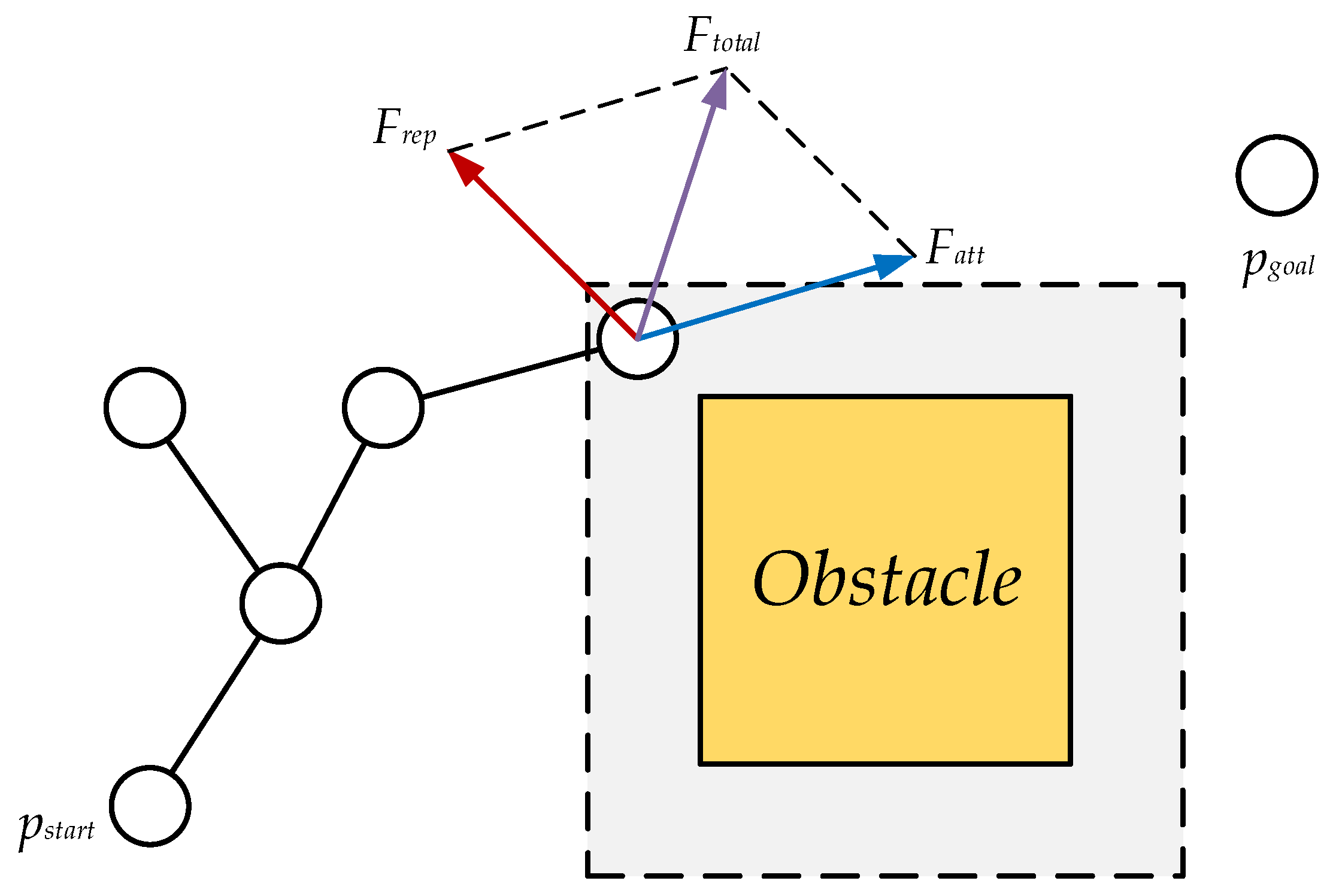
When a vehicle is driving, it will be affected by the joint influence of the gravitational potential field and the repulsive potential field. It is not only affected by the gravitational effect of the target point on it, but also the impact range includes the repulsive force effect of the obstacle where the vehicle is currently located. The combined potential field and combined force effect of the vehicle are shown in the following two formulas.

$$U_{total}\left(d\right)=U_{att}\left(d\right)+\sum _{i=0}^n{U}_{rep}\left(d\right)$$

(5)

$$F_{total}\left(d\right)=F_{att}\left(d\right)+\sum _{i=0}^n{F}_{rep}\left(d\right)$$

(6)

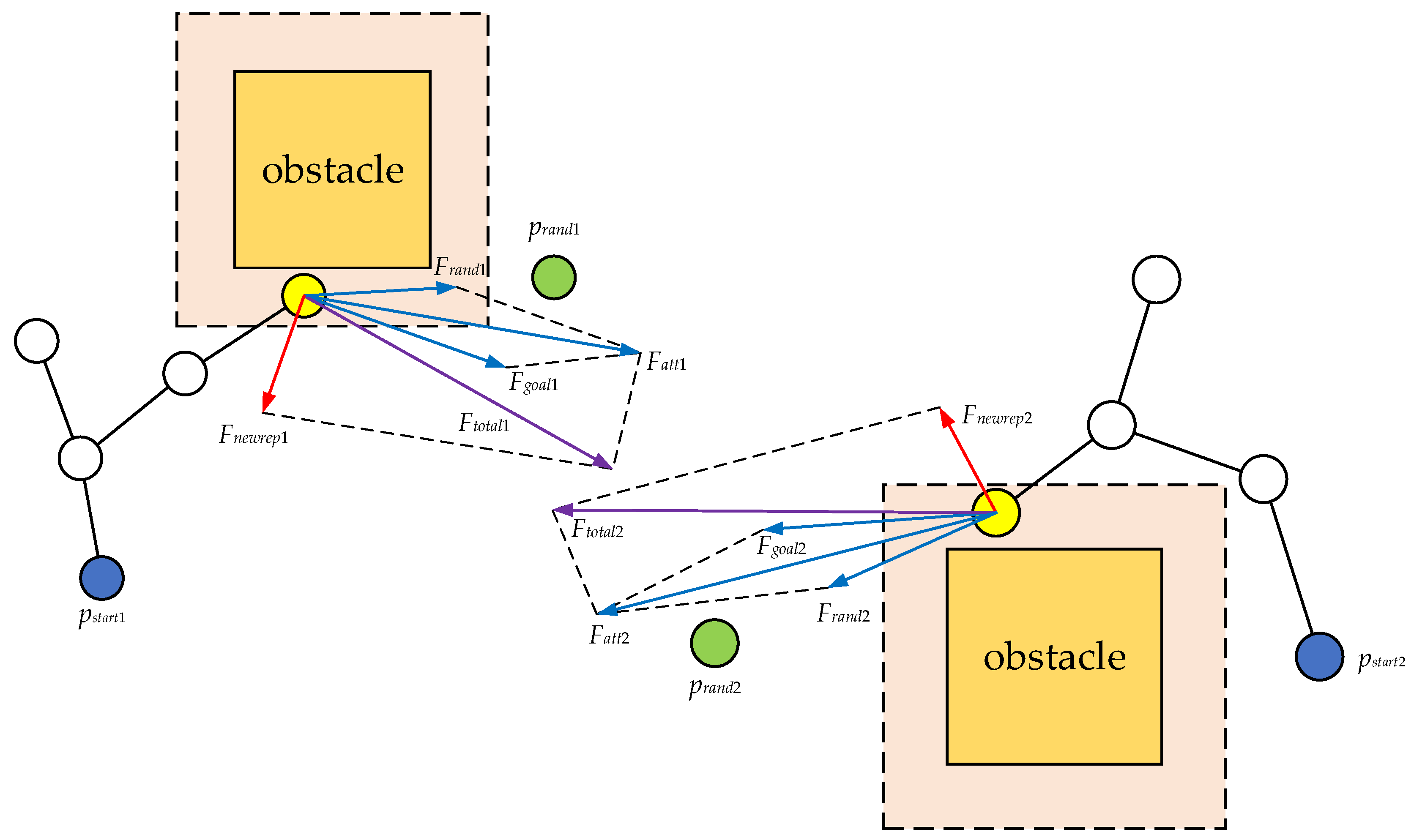
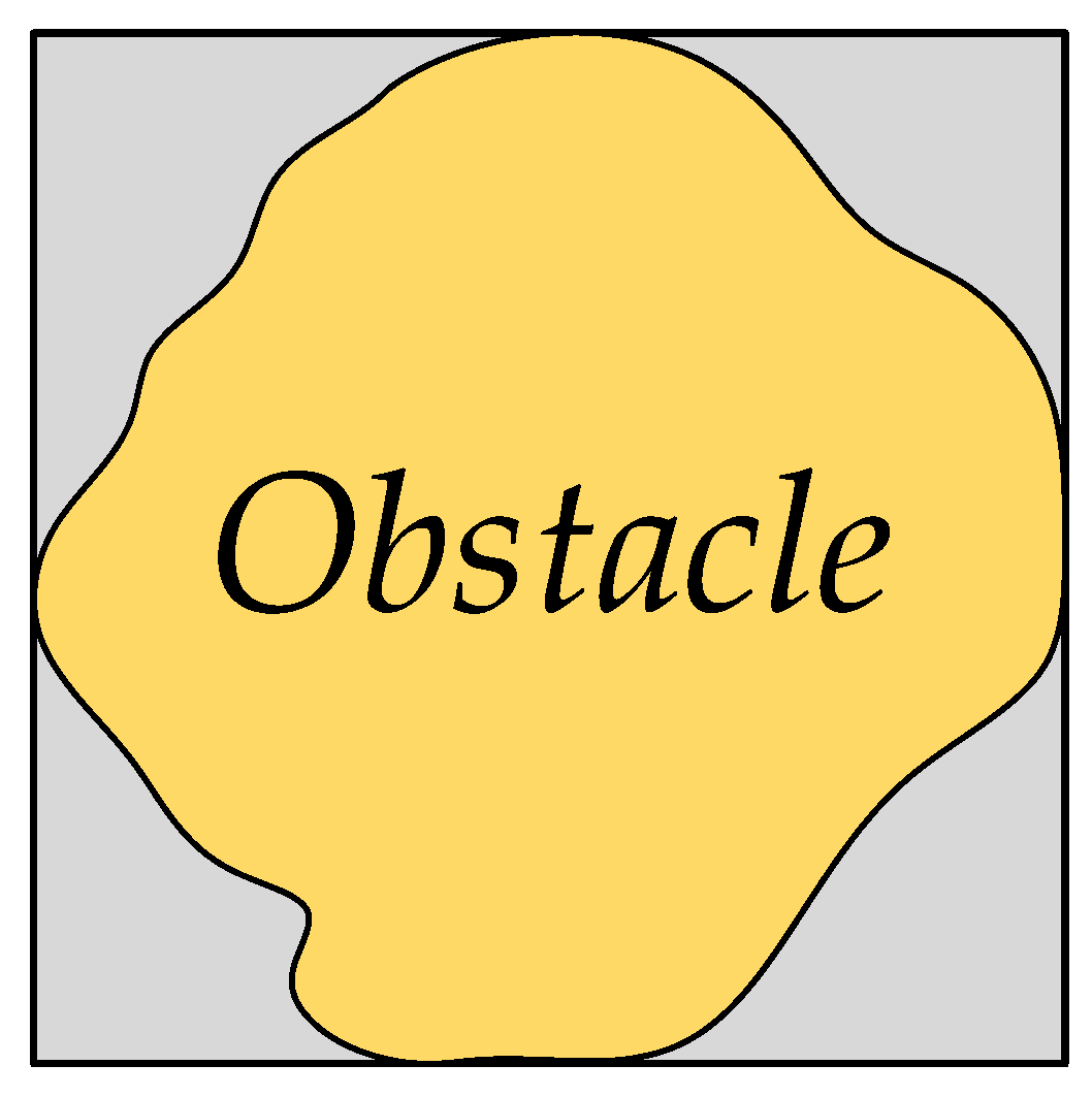
In the formula, $n$ represents the number of obstacles that produce repulsive force on the vehicle at the current position. The algorithm diagram is shownin Figure 5. The gray part in the figure is the influence range of the obstacle. At this time, the node is within the influence range, so it is affected by the repulsion force of this obstacle. The direction of the red arrow is the direction of the repulsion force of the obstacle on the node. At this time, $p_{goal}$ also has a gravitational effect on this node, and the gravitational direction is shown by the blue arrow. The combined force of repulsion and gravity is in the direction of the purple arrow $F_{total}$, and the vehicle will move in this direction.

3. Improved and Fusion Algorithm

3.1. Algorithm Requirements

Compared with the traditional RRT algorithm and RRT* algorithm, the bidirectional RRT* algorithm has the characteristics of fast obtaining global paths and better quality generated paths. Therefore, this paper will use the bidirectional RRT* algorithm as the basic algorithm for fusion improvement so as to quickly obtain global paths [13]. However, for RRT-class algorithms, such algorithms have the problem that sampling too randomly in the global area may cause the target position to be unreachable or waste generated computing power; and for workshop transport vehicles, although such vehicles generally have four-wheel steering capabilities, they still need to be as smooth as possible, which also requires processing the path, with the goal of getting a path with fewer twists and turns. Therefore, the following improvements are made in this paper based on Bi-RRT*.

• Add a target bias strategy to make the algorithm more directional and avoid waste of computing power caused by too random sampling;
• Expand the obstacles and their influence range in the APF algorithm and integrate them into the improved Bi-RRT* algorithm to enhance the algorithm’s obstacle avoidance ability against obstacles and prevent transport vehicles from getting too close or even colliding with obstacles;
• The obtained path is simplified, on the one hand, to reduce path twists and turns to facilitate subsequent smooth global guidance paths, on the other hand, to further shorten the redundant path length caused by random nodes.

3.2. Bi-RRT* Bias Strategy

3.2.1. Common Bias Strategy

The characteristic of RRT algorithms is random sampling, but too much random sampling also leads to extended planning time and wasted computing power. Many random points are meaningless when the actual algorithm is running. Therefore, a target bias strategy is used to guide the random tree so that more new nodes are generated, which is most meaningful for obtaining the global path [14,15,16].

In the process of generating a random tree, a random number $R$ is generated at the same time when generating a random point, and $R$ is required to satisfy the condition $R\in [0,1]$, and then judgment is made on this random number. If the random number $R$ is less than the set bias probability $S$, the next growth direction is the target node $p_{goal}$ which will improve the efficiency of global path acquisition. The schematic diagram of this strategy is shown in Figure 6, which shows two cases of whether bias occurs under the same parent node. The yellow node $p_{new1}$ is a new node generated by taking the direction of the random point $p_{rand}$ as the growth direction without bias, and the green node $p_{new2}$ is a new node generated by taking the direction of $p_{goal}$ as the growth direction due to bias. During the generation process of a bidirectional tree, the global starting point and target point will be used as the target nodes of the opposing tree, respectively. At this time, the two random trees will alternately generate random points $p_{rand1}$ and $p_{rand2}$ and random numbers $R_1$ and $R_2$ and make bias judgments respectively. This operation will improve the growth efficiency of the trees on both sides.

3.2.2. Path Ratio Adaptive Bias Strategy

Although ordinary bias strategies can improve the efficiency of obtaining global paths to a certain extent [17]. However, in practice, this ordinary bias determination is too fixed, and the transportation vehicle may fall into a local optimal state due to insufficient sampling when leaving the current position, resulting in excessive bias, or due to random sampling when approaching the target position. Insufficient bias may lead to the target position but still take a detour and even lead to a wrong path. Therefore, based on the above problems, target bias should be dynamic [18]. This paper proposes an adaptive target biasing strategy based on the path length ratio to solve the problem that over-biasing may occur in the early stage and under-biasing may occur after the route is stabilized.

The bias probability is calculated as follows.

$$P_{bias}=P_{min}+(P_{max}-P_{min})\times (1-e^{-k·R_{distance}})$$

(7)

$$R_{distance}={\displaystyle \frac{d_{cost}}{d_{total}}}$$

(8)

In Equation (7), $P_{bias}$ represents the random probability of possible bias, $P_{min}$ represents the minimum bias probability, $P_{max}$ represents the maximum bias probability, $k$ is an adjustment parameter and $0<k\le 1$, and its value controls the growth rate of bias probability; $R_{distance}$ is the path ratio; $d_{cost}$ in Equation (8) refers to the total cost from the starting node to the current node position; and $d_{total}$ is the estimated total path length, and its value is the Euclidean distance between the starting point and the target point.

During the node generation process, since the node is not generated in the initial state, the total cost $d_{cost}=0$, so $P_{bias}=P_{min}$ at this time, and node generation will take the minimum bias probability as the determination condition. If the random number generated at this time is lower than the determination condition and $R_{distance}=0$ at this time, it is considered that the current node generation is still within an initial range. At this time, the growth direction can be set to the direction of the target node $p_{goal}$. Since the probability is small, at this time, the bias plays a role in guiding future trends, and the random points play a greater role in tree generation, which reduces the possibility of falling into a local optimal; but as the planning continues, $R_{distance}$ will continue to increase. At this time, it is believed that the transport vehicle has left the original position, and the $P_{bias}$ at this time also continues to increase. The bias probability in the $p_{goal}$ direction increases as the growth direction gradually increases, which better guides the tree to move towards the target node and reduces path waste. The pseudocode for the adaptive bias strategy based on path ratio is shown in Algorithm 4.

Algorithm 4. Path Ratio Adaptive Bias Strategy
1:	Define  $P_{min},P_{max},k$
2:	$d_{cost}\leftarrow PathCost\left(p\right)$
3:	$d_{total}\leftarrow \parallel p_{start}-p_{goal}\parallel$
4:	$R_{distance}\leftarrow d_{cost}/d_{total}$
5:	$P_{bias}\leftarrow P_{min}+(P_{max}-P_{min})(1-e^{-k{·R}_{distance}})$
6:	$P_{bias}\leftarrow \mathrm{m}\mathrm{a}\mathrm{x}(P_{min},\mathrm{m}\mathrm{i}\mathrm{n}(P_{bias},P_{max}\left)\right)$
7:	if  $rand\left(\right)<P_{bias}$ then
8:	$p_{sample}\leftarrow p_{goal}$
9:	else
10:	$p_{sample}\leftarrow p_{rand}$
11:	end if
12:	$p_{new}\leftarrow \mathrm{E}\mathrm{x}\mathrm{t}\mathrm{e}\mathrm{n}\mathrm{d}\mathrm{t}\mathrm{r}\mathrm{e}\mathrm{e}\left(T,p_{sample},\delta ,Obs\right)$
13:	return $p_{new}$

3.3. Obstacles Expansion Strategy

The APF algorithm is often introduced into RRT-class algorithms to guide random trees to generate and avoid obstacles [19,20]. However, although the APF algorithm can use repulsive force to keep nodes away from obstacles, in actual situations, especially for moving machines with large entities such as vehicles, such simple repulsive force generally cannot avoid obstacles well. Therefore, this paper proposes that the concept of safe distance can be used to expand obstacles [21]. Increase the obstacle area and influence range to enhance the repulsion effect in the APF algorithm.

Before the expansion processing, irregular obstacles should first be regularized. The processing method is as shown in Figure 7. This method uses the maximum outer diameter of the irregular obstacle to obtain its circumscribed rectangle, and the rectangle represents the irregular obstacle. The gray part in Figure 7 is the extra obstacle part after the irregular obstacle is regularized.

This kind of method is simple, efficient, and in line with engineering practice. For example, in workshop scenarios, a safe distance range is often established between the road and the equipment or pile, which can be regarded as an equipment safety area, that is, a kind of external expansion of obstacles. In Figure 8a, $a$ is the safety distance, the value of which ranges from $a\ge 0$. The setting of the safety distance size in the planning process will affect how far the path is kept away from the obstacle; the larger the value, the greater the range of influence of the obstacle on the vehicle, and it will extend an area around the obstacle that also cannot be collided with. the yellow part represents the initial size of the obstacle; the gray range within the black dotted line is the range in which the obstacle can originally exert repulsive force; the red area within the red dotted line is the area of the expanded obstacle, and the expanded part is determined by the safety distance; and the green area within the green dotted line is the range of the obstacle’s repulsive force increased by the expanded obstacle compared to the original obstacle, and the expansion size is also determined by the safety distance. As shown in Figure 8b, after the obstacle expands, the generation node will be affected by repulsive force within the new influence range, and when detecting the obstacle, if it collides with the expanded obstacle area, it will also be regarded as a collision with the obstacle. This strategy makes it difficult to get closer to the obstacle or even interfere with the obstacle when generating the path. When applied to the planning of mobile machinery such as vehicles, the safety distance can be set to be greater than 0.5 times the maximum outer size of the vehicle so that the vehicle can be virtually simplified into a particle during the planning process. The obstacle inflation strategy can further improve the obstacle avoidance ability of the algorithm and make the planned path far away from obstacles.

3.4. Fusion Improvement Algorithm

In the fusion algorithm of the RRT algorithm and the APF algorithm, the method of applying a gravitational potential field at the target point and a repulsive potential field on the obstacle is commonly used [22,23]. For the Bi-RRT* algorithm, since it uses a bidirectional random tree to generate a complete global path, the application of the gravitational potential field should be applied to the initial nodes $p_{start1}$ and $p_{start2}$ on both sides. For the random points generated by the target bias strategy, it also has the effect of guiding node generation in the Bi-RRT* algorithm. The adaptive target bias strategy proposed in this paper can also avoid the situation that nodes fall into local optima and the target position cannot be reached to a certain extent in the process of bi-directional node generation. Therefore, the generated random point $p_{rand}$ should also have a gravitational effect and comprehensively guide node generation. The combined gravity exerted on the current node is the resultant force of the gravity of the starting node of another tree and the gravity of the random point generated by its tree. The formula is as follows.

$$F_{att}\left(d\right)=F_{goal}\left(d\right)+F_{rand}\left(d\right)$$

(9)

In the above formula, $F_{att}\left(d\right)$ is the combined gravity exerted on the current node, $F_{goal}\left(d\right)$ refers to the gravity exerted on the current node by the target point corresponding to the random tree where the current node is located, and $F_{rand}\left(d\right)$ refers to the gravity exerted by the random point.

During the process of generating nodes between the two random trees, the expanded obstacles around them will produce repulsive forces within the influence range of their expanded repulsive forces. The two nodes will be affected by the repulsive force of these obstacles, and the generated new node $p_{new}$ will be subjected to collision detection with the expanding obstacle when generating the tree, so that collisions with obstacles can be avoided during the node generation process. The formula is expressed as follows.

$$F_{rep}\left(d\right)=\sum _{i=0}^n{F}_{newrep}\left(d\right)$$

(10)

In Equation (10), $F_{rep}\left(d\right)$ is the repulsive force of obstacles encountered by the current node, $n$ represents the number of obstacles that can affect the current node, and $F_{newrep}\left(d\right)$ is the repulsive force exerted by the expanded obstacles.

In Figure 9, the orange square and its outer dotted line range are the influence range of the expanded obstacle and the expanded repulsion force. The green nodes are the random nodes $p_{rand1}$ and $p_{rand2}$ generated by the trees on both sides, respectively. The blue node is the starting point and target point of the global path and also the starting points $p_{start1}$ and $p_{start2}$ of the two random trees, respectively. The yellow node is the current node. Both yellow nodes in the figure are within the influence range of the obstacle repulsion force at this time. Therefore, they are each subjected to repulsive forces $F_{newrep1}$ and $F_{newrep2}$, with the direction of repulsive forces as shown by the red arrows in the figure, and under the double attraction of the random point gravity and the target point gravity, they are respectively subjected to the combined attractive forces $F_{att1}$ and $F_{att2}$, with the directions as shown by the blue arrows. Under the action of the resultant forces $F_{total1}$ and $F_{total2}$, new nodes are guided and generated in the direction of the purple arrow. The calculation method of the resultant force is still as shown in Equation (6).

3.5. Path Optimization Strategy

In the above, the Bi-RRT* algorithm has been improved and integrated to enhance the efficiency and guidance of node generation. However, after the path is generated, since node generation is still accompanied by certain randomness, the path is still relatively tortuous. For transportation vehicles, although most vehicles have certain four-wheel steering capabilities, too tortuous paths still do not conform to the vehicle’s kinematic laws, and too dense and random nodes are difficult to ensure the quality of the smoothed path in post-processing. Therefore, path optimization is needed.

In this paper, the redundant node deletion strategy [24] is used to optimize the resulting global path, and its pseudocode is shown in Algorithm 5.

Algorithm 5. Redundant Node Deletion Strategy
1:	$P\leftarrow \{p_1,p_2,\dots ,p_n\}$
2:	$P_{opt}\leftarrow \left\{p_1\right\}$
3:	$i\leftarrow 1$
4:	while $i<n$do
5:	$\mathit{j}\leftarrow \mathit{n}$
6:	while $j>i+1$ do
7:	if  $\mathrm{C}\mathrm{o}\mathrm{l}\mathrm{l}\mathrm{i}\mathrm{s}\mathrm{i}\mathrm{o}\mathrm{n}\mathrm{C}\mathrm{h}\mathrm{e}\mathrm{c}\mathrm{k}(p_i,p_j,Obs)\leftarrow False$ then
8:	break
9:	else
10:	$j\leftarrow j-1$
11:	end if
12:	end while
13:	if $\mathit{j}>i$ then
14:	$P_{opt}\leftarrow P_{opt}\cup \left\{p_j\right\}$
15:	$i\leftarrow j$
16:	else
17:	$i\leftarrow i+1$
18:	end if
19:	end while
20:	return  $P_{opt}$

This strategy adopts the idea of a greedy algorithm, starting from the initial node of the global path and connecting to the furthest node. If the connection line collides with the obstacle when connecting to the end node, it falls back to the previous node. If there is still a collision, it returns to another node until there is no collision between the node and the initial node. The two nodes are directly connected, and all points between the two nodes are deleted in the node set of the path random tree. Since the obstacles were expanded before, the overall path will be far away from the obstacles, which also provides convenience for redundant node deletion and can better shorten the total path length. Repeat the above steps until all nodes complete the traversal.

In Figure 10a, the dotted line part is the process of filtering during the traversal of nodes. The red dotted line is caused by collision with an obstacle, resulting in the failure of redundant node deletion. When traversing to node 4, the obstacle collision detection condition is met. Therefore, the direct connection between node 1 and node 4 is represented by a blue dotted line in the figure. Similarly, the determination condition for redundant node deletion is met between node 4 and node 6, so it is directly connected. In Figure 10b, the solid blue line represents the direct connection path after node deletion, and the dotted line is the original path for deletion, which shows that it generally shortens the path length and reduces the path turning. As the redundant nodes between two directly connected nodes are removed, the redundant length of the paths and the turning points are also reduced, which overall shortens the redundant path lengths and redundant path turns in the global paths due to the random sampling process.

3.6. Path Smoothing Processing

For small intelligent transport vehicles, to ensure convenient transportation and space adaptability, they generally have the function of four-wheel steering. Although the algorithm uses the strategies such as obstacle avoidance and redundant node deletion in the previous article, the global path obtained by the transport vehicle does not meet the vehicle kinematics and cannot meet its smooth driving. Therefore, it is necessary to perform smooth optimization processing on the paths obtained by the algorithm.

3.6.1. Bezier Curve Processing

The path smoothing is performed using the n-order Bezier curve. Since the redundant node was deleted in the previous algorithm, if only the starting point and target point of the current section path remain after the path deletes the node, the algorithm will not perform Bezier smoothing calculations to reduce waste of computing power. Otherwise, the path will be smoothed with the remaining nodes after the delete as the control node. The Bezier curve formula is as follows.

$$P_n\left(t\right)={\sum }_{i=0}^n{B}_{i,n}\left(t\right)·P_i,t\in [0,1]$$

(11)

$$B_{i,n}\left(t\right)={\sum }_{i=0}^n{t}^i{(1-t)}^{n-i}{\displaystyle \frac{n!}{i!\left(n-i\right)!}}$$

(12)

In the above two formulas, $B_{i,n}\left(t\right)$ is the Bernstein basis function, representing the n-order Bezier curve determined with $P_0$ and $P_n$ as the starting point and the end point, the point between the two is the intermediate control point, and $P_i$ represents the control point. In the process of global path smoothing, the resulting path is discretized by inserting segmented nodes, and the discretized path points are calculated as control points to obtain Bezier curve points. Connect these points to get a complete path.

3.6.2. Potential Field Auxiliary Node Strategy

Since the above-mentioned redundant node deletion strategy is added to the algorithm, the redundant nodes are deleted, which shortens the path length, but the number of control points of its path is also reduced. For Bezier curve smoothness, collision with obstacles may occur due to fewer control nodes. In order to avoid path distortion caused by path smoothing, this paper proposes a potential field auxiliary node strategy: insert auxiliary nodes based on the obstacle repulsive force potential field at the path turning point to ensure that the turning point fits into the pre-planned path and prevents path distortion.

In the above, when redundant nodes are deleted, it was found that the path turning point is generally a sharp point, and in the process of smoothing the Bezier curve, such sharp points will be regarded as control points, which will cause the turning position to bend the inner side of the Bezier than the turning point, which is also a reason for path distortion and collision. Therefore, the insertion auxiliary node should be near the bend point, and the repulsive potential field idea should be integrated to find the obstacle closest to the turning node, and initially determine that this obstacle has a repulsive effect on the turning point, and then determine whether the repulsive force range of the obstacle covers this node. If it has been covered, then the repulsive force affects this node and will have a repulsive effect on the node. The pseudocode of potential field auxiliary node strategy is shown in Algorithm 6.

Algorithm 6. Potential Field Auxiliary Node Strategy
1:	$P_{aux}\leftarrow \left\{p_1\right\}$
2:	for  $i=1ton-1$ do
3:	$p_{current}\leftarrow p_i$
4:	$p_{next}\leftarrow p_{i+1}$
5:	for all $obs\in Obs$ do
6:	$d_{current}\leftarrow \mathrm{D}\mathrm{i}\mathrm{s}\mathrm{t}\mathrm{a}\mathrm{n}\mathrm{c}\mathrm{e}(p_{current},obs)$
7:	if $d_{current}\le d_{req}$ then
8:	$\stackrel{⃑}{F_{req}}\leftarrow -k_{req}\nabla {\displaystyle \frac{1}{d_{current}}}$
9:	for ${\theta }_{offset}\in A\theta ,A\in \left[-a,a\right]\cap A,a\in Z$ do
10:	$\stackrel{⃑}{F_{aux}}\leftarrow \mathrm{R}\mathrm{o}\mathrm{t}\mathrm{a}\mathrm{t}\mathrm{e}(\stackrel{⃑}{F_{rep}},{\theta }_{offset})$
11:	$p_{aux}\leftarrow p_{current}+s_{aux}·\stackrel{⃑}{F_{aux}}$
12:	if $\mathrm{C}\mathrm{o}\mathrm{l}\mathrm{l}\mathrm{i}\mathrm{s}\mathrm{i}\mathrm{o}\mathrm{n}\mathrm{C}\mathrm{h}\mathrm{e}\mathrm{c}\mathrm{k}(p_i,p_j,Obs)\leftarrow False$ then
13:	$P_{aux}\leftarrow P_{aux}\cup \left\{p_{aux}\right\}$
14:	end if
15:	end for
16:	end if
17:	end for
18:	$P_{aux}\leftarrow P_{aux}\cup \left\{p_{next}\right\}$
19:	end for
20:	return  $P_{aux}$

In the repulsive force direction, an auxiliary point is generated with a small step size $s_{aux}$. In the direction where the angle offset of both sides of the repulsive force direction is $\theta$, each interval $\theta$, an auxiliary node is generated with a small size step $s_{aux}$, and auxiliary nodes are generated symmetrically on both sides. The generation of auxiliary points can also be understood as making an arc with the turning node as the center and the small size step $s_{aux}$ as the radius, which takes the repulsive force direction as the axis of symmetry. For example, as shown in Figure 11, the figure is set with 5 auxiliary points, and the center angle corresponding to the arc is $4\theta$. The intersection point of this section of arc and $A\theta ,A\in [-2,2]\cap A\in Z$ is the auxiliary point position. The schematic diagram is as follows.

The set auxiliary points and other path points are used as the control points for smooth Bezier curves, and the resulting path curve is more in line with the original path, effectively preventing problems such as obstacle collision caused by path distortion.

4. Multi-Target Planning Strategy

4.1. Multi-Target Demand Analysis

In indoor transportation scenarios, such as transportation within workshops and component distribution transportation, the delivery of materials often involves multiple receiving locations, and during the transportation process, these target locations need to be traversed. There are various ways to traverse the targets. Generally speaking, the planning methods for traversing each target point can be roughly divided into two categories: predefined sequence traversal and non-predefined sequence traversal. In predefined sequence transportation planning, the route typically follows the structure of “starting position → target location 1 → target location 2 → ... → target location N → starting position,” where the traversal order of target locations is predetermined and requires no further sequencing during subsequent planning. In contrast, non-predefined sequence transportation planning adopts the route pattern of “initial position → target location 1 → target location 2 → ... → target location N → initial position.” Here, the delivery sequence of target locations is not initially constrained, but the vehicle must return to the initial position after completing all deliveries to prepare for subsequent tasks. Consequently, the optimal traversal sequence of target points requires computational optimization to determine. Since the traversal order in predefined sequence transportation is fixed, current algorithmic research primarily focuses on non-predefined sequence transportation strategies, which dynamically optimize path planning without relying on predefined prioritization of target locations.

4.2. Planning 1: Predefined Sequence Planning

In predefined sequence transportation, the vehicle follows a human-defined traversal order of target nodes. This transportation mode is typically employed in scenarios such as workpiece transfer between processes within factory workshops. Its primary characteristic lies in requiring the vehicle to traverse multiple work areas strictly according to a predetermined target sequence, without considering optimization requirements like route length minimization. The algorithmic focus resides in generating compliant paths that adhere to the prescribed traversal sequence.

In predefined sequence transportation algorithms, no sorting operation is required for the target node list. Instead, the global path is generated by sequentially planning routes to each target node in the predefined order. Starting from the initial position, the algorithm iteratively plans paths to each target node according to their sequence in the list. Upon reaching a target node, the subsequent node in the list is designated as the new current target, with the current node’s position serving as the local starting point for the next path planning iteration. This process continues until all target nodes in the list are traversed. Finally, a return path is planned from the last target node back to the global starting position. For example, indoor transportation vehicles, which are typically equipped with four-wheel steering functionality, must deliver materials to fixed target zones with precise positioning. Consequently, path smoothing algorithms are applied only to in-transit segments to ensure vehicle stability during movement, while the final approach paths at target locations remain unmodified to guarantee delivery accuracy. A schematic diagram of ordered transportation is illustrated below.

In Figure 12, the planning process begins at $p_{start}$, with all other points designated as target nodes to be sequentially traversed according to their predefined order. The planning flow direction, as illustrated by the blue arrows in the diagram, follows a mechanistic decision-making framework, where the algorithm rigidly adheres to the input sequence of target nodes during global path generation. While this approach guarantees compliance with the predefined order, it risks suboptimal efficiency in scenarios requiring cost-sensitive operations. For example, if the nodes are irregularly distributed, the accumulation of locally inefficient path segments (e.g., redundant detours or backtracking) may result in a substantially increased total path length.

4.3. Planning 2: Local Shortest Planning Strategy

In contrast to predefined sequence transportation, non-predefined sequence transportation aggregates all target points to be traversed into a single target node list, imposing no specific constraints on the traversal order of locations. Its primary objective is to minimize the total travel distance, thereby enhancing efficiency.

The local shortest path planning strategy is a simplified approach for prioritizing target nodes, emphasizing traversal efficiency by iteratively selecting the nearest unvisited node (i.e., a local optimal solution) to reduce the global path length. After traversing all target nodes in the list, the vehicle returns to the initial position. In this algorithm, a greedy algorithm [25] is employed to dynamically prioritize target nodes. The process involves iteratively checking unvisited nodes in the goal list, calculating inter-node distances, and selecting the closest unvisited node as the next destination. The current node is then marked as visited, and this cycle repeats until all targets are traversed. Finally, a feasible return path from the last target node to the global initial position is generated. By selecting the nearest unvisited target point, this strategy attempts to approximate a shorter global path, albeit potentially suboptimal due to its myopic focus on local minima. A schematic of this planning strategy is shown in Figure 13a, and the pseudocode for the strategy is provided in Algorithm 7.

Algorithm 7. Local Shortest Planning Strategy
1:	$V\leftarrow \{p_{goal1},p_{goal2},\dots ,p_{goal\mathrm{n}}\}$
2:	$visited\left[p_{goal}\right]\leftarrow False,\forall p_{goal}\in V$
3:	$Order\leftarrow \left[\right]$
4:	$p_{current}\leftarrow p_{start}$
5:	while  $\exists p_{goal}\in V\bigwedge visited\left[p_{goal}\right]=False$ do
6:	$unvisited\leftarrow \{p_{goal}\in V|visited\left[p_{goal}\right]=False\}$
7:	$next\leftarrow {\mathrm{a}\mathrm{r}\mathrm{g}\mathrm{m}\mathrm{i}\mathrm{n}}_{p_{goal}\in unvisited}\mathrm{S}\mathrm{h}\mathrm{o}\mathrm{r}\mathrm{t}\mathrm{e}\mathrm{s}\mathrm{t}(p_{current},p_{goal})$
8:	$visited\left[next\right]\leftarrow True$
9:	$Order\leftarrow Order\cup \left\{next\right)\}$
10:	$p_{current}\leftarrow next$
11:	end while
12:	$Order\leftarrow Order\cup \left\{p_{start}\right)\}$
13:	return $Order$

However, the disadvantage of the algorithm is that it pays too much attention to the shortest local path and ignores the global path length. The reason is that although each local shortest plan can traverse the closest target node to the current target node as the next planning object, if the target points are not uniform, the shortest possible target nodes may be insufficient in the second half of the sorting, resulting in the last few planning distances or the final planning target point away from the initial position. This method is also prone to path intersections and redundant detours, causing waste of path length.

In Figure 13a, the dark blue and light blue dotted and solid lines determine the distance of each unvisited target point from the starting point $p_{start}$ where $p_{goal4}$ is the closest distance, so $p_{goal4}$ will become the first target point. Continue to make the shortest distance judgment, use $p_{goal4}$ as the current node to traverse other unvisited nodes, and $p_{goal3}$ is the closest target node, so $p_{goal3}$ will become the next target node; repeat the above operation to traverse all target nodes. The last node is $p_{goal2}$. Since all target nodes have been accessed, a path returning to the global starting point $p_{start}$ will be planned from $p_{goal2}$. The final global path is $p_{start}\to p_{goal4}\to p_{goal3}\to p_{goal1}\to p_{goal2}\to p_{start}$.

The final obtained path is shown in Figure 13b. It is obvious that although the local path is guaranteed to be the shortest when traversing all target points, when returning to the global start point $p_{start}$ the planned path intersects with other paths and the planning direction of $p_{goal1}\to p_{goal2}$ is far away from the starting target point. This intersection or uneven target position on the path may cause waste on the overall path, resulting in the shortest local path each time, because the redundancy length is large, the global path is still long, and the turning angle on the global path may be too large, which makes it difficult for the vehicle to drive.

4.4. Planning 3: Heuristic Planning Strategy

The local shortest planning strategy described above can improve the efficiency of the algorithm for target node traversal to a certain extent, and realize that by selecting the nearest target node to visit all target positions and returning to the initial position at the end, but in some scenarios where the distribution of target positions is not uniform and the path order has a great impact on the global path, the node order after the local shortest planning strategy is sorted may not be able to plan the shorter global paths. The main reason is that when the local distance is shorter, the advantages and disadvantages of the global path are ignored because too much attention is paid to the local solution as the optimal solution. Therefore, a sorting strategy is needed to ensure robustness while also being able to obtain shorter global paths faster.

This paper proposes a heuristic planning strategy. The basis of this strategy still uses the idea of greedy algorithms to traverse nodes. The main goal of this strategy is to select the next untraversed target point that is most likely to make the global path shortest under the premise of avoiding collisions. For this purpose, a comprehensive scoring system is designed to measure the pros and cons of each unvisited target point. Since the main waste of time and iterative waste during vehicle driving or algorithm sampling is caused by excessively long paths or excessively large direction changes [26], the heuristic scoring formula combines distance weights and angle weights to avoid unnecessary detours of the path and optimizes the overall path length.

This strategy first calculates the Euclidean distance from the global start point to each target point and selects the first target point by comparing the distance between all target points and the global start point. For other unvisited target points, the sorting method is performed using a heuristic planning strategy, mainly calculating the distance between the unvisited target points and the current target points, as well as the comprehensive weight of the vector angle calculation scores, and updating the planning order. For unvisited target nodes, their distance and angle calculation methods are shown in the following formula.

$$d=\parallel p_{goal}-p_{current}\parallel$$

(13)

$$\mathrm{c}\mathrm{o}\mathrm{s}\left(\theta \right)={\displaystyle \frac{(p_{current}-p_{start})·(p_{goal}-p_{current})}{\parallel p_{current}-p_{start}\parallel ·\parallel p_{goal}-p_{current}\parallel }}$$

(14)

$$\theta =\mathrm{a}\mathrm{r}\mathrm{c}\mathrm{c}\mathrm{o}\mathrm{s}(\mathrm{c}\mathrm{o}\mathrm{s}(\theta ))\times {\displaystyle \frac{180°}{\pi }}$$

(15)

In the above three formulas, $d$ is the Euclidean distance between the current node and the target node, and $\theta$ is the angle between the current target point and the vector from the current target point to the next potential target point. To prevent data exceptions during the calculation process, the included angle needs to be normalized, and the included angle is controlled to be between 0 and 180°. The method is as follows.

$$\theta =\mathrm{a}\mathrm{r}\mathrm{c}\mathrm{c}\mathrm{o}\mathrm{s}(\mathrm{m}\mathrm{a}\mathrm{x}(\mathrm{m}\mathrm{i}\mathrm{n}\left(\mathrm{c}\mathrm{o}\mathrm{s}\left(\theta \right),1\right),-1)\times {\displaystyle \frac{180°}{\pi }}$$

(16)

Next, comprehensive weight calculation is performed, and the heuristic weight calculation formula is as follows.

$${score}_i={\omega }_d·d+{\omega }_{\theta }·\theta$$

(17)

In Equation (17), ${score}_i$ represents the comprehensive score of the i-th target node, ${\omega }_d$ is the distance weight value of the node, and ${\omega }_{\theta }$ is the angle weight value of the node. The pseudocode of the heuristic planning strategy is shown in Algorithm 8.

Algorithm 8. Heuristic Planning Strategy
1:	$V\leftarrow \{p_{goal1},p_{goal2},\dots ,p_{goal\mathrm{n}}\}$
2:	$visited\left[p_{goal}\right]\leftarrow False,\forall p_{goal}\in V$
3:	$Order\leftarrow \left[\right]$
4:	$p_{current}\leftarrow p_{start}$
5:	$d_{start}\leftarrow \mathrm{D}\mathrm{i}\mathrm{s}\mathrm{t}\mathrm{a}\mathrm{n}\mathrm{c}\mathrm{e}\left(p_{start},p_{goal}\right),\forall p_{goal}\in V$
6:	${idx}_{min}\leftarrow \mathrm{a}\mathrm{r}\mathrm{g}\mathrm{m}\mathrm{i}\mathrm{n}\left(d_{start}\right)$
7:	$Order\leftarrow Order\cup \left\{p_{goal}\right({idx}_{min}\left)\right\}$
8:	$visited\left[next\right]\leftarrow True$
9:	while  $\exists p_{goal}\in V\bigwedge visited\left[p_{goal}\right]=False$ do
10:	$unvisited\leftarrow \{p_{goal}\in V|visited\left[p_{goal}\right]=False\}$
11:	$next\leftarrow {\mathrm{a}\mathrm{r}\mathrm{g}\mathrm{m}\mathrm{i}\mathrm{n}}_{p_{goal}\in unvisited}Shortest(p_{current},p_{goal})$
12:	$visited\left[next\right]\leftarrow True$
13:	$Order\leftarrow Order\cup \left\{next\right)\}$
14:	$p_{current}\leftarrow next$
15:	end while
16:	$Order\leftarrow Order\cup \left\{next\right)\}$
17:	return $Order$

After all global goal points are sorted, the path between every two goal points is planned using the fusion improvement algorithm described above and connected to each other to obtain a complete and global path that can return to the global initial position. For the transportation vehicle, it needs to stay at the predefined target location to wait for the handling and storage of goods, and it generally has the function of turning in place, which has the need for accuracy for the target location, so the positioning path at each target point is not required to be additionally smoothed to ensure that the vehicle can arrive at the predefined target location. The flowchart of the overall planning process for planning a global path using heuristic planning strategies is shown in Figure 14.

5. Simulation Verification

5.1. Fusion Improved APF and Improved Bi-RRT* Algorithm Simulation Analysis

To verify and analyze whether the algorithm that combines APF and improved Bi-RRT* in this paper can effectively search target points in the map to form a global path, the algorithm in this paper is simulated and verified in several environments. The simulation environment is MATLAB R2022b, and the map is a 2D map of 100 × 100. The global starting node is (10, 10), the global target node is (90, 90), the maximum number of algorithm iterations is 2000, the random tree growth step is 2, the expansion safety distance is 1, the artificial potential field gravitational coefficient is 1.0, the repulsive force coefficient is 0.9, the safety distance is 2, and the repulsive force influence range is 15. In the map, the green solid node represents the starting node, and the red solid node represents the target node. When a one-way random tree is used, blue nodes and blue lines represent the nodes grown by the random tree and the random tree. When a bidirectional random tree is used, another tree is represented by pink lines and pink nodes. Finally, the global path from the start point to the target point is represented by the green solid line. In the comparative analysis, three types of maps were used, and the area of obstacles accounted for 10%, 15%, and 20% of the total map, and their density represented the general environment, general complex environment, and complex environment, respectively. When analyzing the algorithms in this article, the comparison algorithms are RRT algorithms, RRT* algorithms, improved RRT* algorithms with fixed biases, improved APF-RRT* algorithms, and Bi-RRT* algorithms.

5.1.1. Simulation Experiment 1

According to the data in

Table 3. Data comparison in map 1.

Algorithm Name	Average Iterations	Average Path Length (m)	Average Time Consumption (s)
RRT	548.40	146.10	10.23
RRT*	503.05	143.82	9.49
Improved RRT*	218.25	136.99	4.68
Improved APF-RRT*	165.10	122.54	2.75
Bi-RRT*	155.30	143.87	1.64
The algorithm in this article	86.80	119.61	0.80

, the fusion improvement algorithm in this paper reduces the number of iterations compared with RRT, RRT*, Improved RRT*, Improved APF-RRT*, and Bi-RRT* in the environment of map 1 by 84.2%, 82.7%, 60.2%, 47.4%, and 44.1%, respectively, compared with other algorithms in the path length by 18.1%, 16.8%, 12.7%, 2.4%, and 16.9%, respectively, while in terms of average time spent, the algorithm in this paper reduces the number of iterations by 92.2%, 91.6%, 82.9%, 70.9%, and 51.2% compared with other comparison algorithms, respectively. It is also worth mentioning that during the comparison process, it was found that the three algorithms, RRT, RRT* and Improved RRT*, sampled in the global scope and could correctly obtain the global path. However, the iteration efficiency was average. The Improved APF-RRT* algorithm occasionally fell into a local optimal situation when encountering obstacles between certain starting points and target points. This lengthened the time spent on the algorithm and caused waste in search iteration. The Bi-RRT* algorithm iterated faster, but the acquisition path was longer, which was related to the randomness of its bidirectional growth random tree. The fusion improvement algorithm proposed in this article, due to the addition of random point gravity and adaptive bias strategies, not only can the local optimal situation be avoided to a certain extent, but it is easier to connect two opposite random trees with a higher success rate than Bi-RRT*. Moreover, the paths planned by RRT, RRT*, Improved RRT*, and Bi-RRT* can be seen in Figure 15 to have many twists, and the paths are closer to the obstacles and are prone to danger. The fusion improvement algorithm proposed in this article, due to the addition of the safe distance for the obstacle expansion, makes the planned paths away from the obstacles, and after applying the redundant point deletion strategy, it can still maintain a short global path.

5.1.2. Simulation Experiment 2

Map 2 is more complex than the Map 1 environment. According to the data in

Table 4. Data comparison in map 2.

Algorithm Name	Average Iterations	Average Path Length (m)	Average Time Consumption (s)
RRT	558.70	148.30	11.85
RRT*	519.60	147.99	10.73
Improved RRT*	254.00	136.43	5.74
Improved APF-RRT*	282.50	121.12	6.79
Bi-RRT*	188.75	152.98	2.33
The algorithm in this article	91.00	119.60	1.03

, the number of iterations of the fusion and improvement algorithm in this article has decreased by 83.7%, 82.5%, 64.2%, 67.8%, and 51.8% compared with RRT, RRT*, Improved RRT*, Improved APF-RRT*, and Bi-RRT*, respectively, and the overall optimization degree is relatively obvious, while in terms of path length, it has decreased by 19.4%, 19.2%, 12.3%, 1.3%, and 21.8%, respectively, and 91.3%, 90.4%, 82.1%, 84.8%, and 55.8%, respectively, in time spent. Compared with the other five algorithms, the algorithms integrated and improved in this paper have a better optimization degree in more complex environments. The three algorithms, RRT, RRT* and Improved RRT*, have relatively stable path acquisition capabilities and are less affected by the environment. The search efficiency of the Improved APF-RRT* algorithm in such more complex environments is much lower than that in simple environments. Although it can ensure that the path is shorter, the iteration time and iteration times have increased. Due to its strong bidirectional randomness, the Bi-RRT* algorithm has fewer iterations and takes less time than RRT* and Improved RRT*, but the global path obtained is longer. This paper combines the improved algorithm. In this environment, not only does it have the bidirectional fast advantage of Bi-RRT*, but it also has a significant reduction in the number of iterations and iteration time. It can also be seen in Figure 16, and the generated path is also good, and it can still maintain a safe distance from obstacles in this environment.

5.1.3. Simulation Experiment 3

Map 3 is a complex map, and its obstacle area accounts for about 20% of the total map area. According to the data in

Table 5. Data comparison in map 3.

Algorithm Name	Average Iterations	Average Path Length (m)	Average Time Consumption (s)
RRT	640.10	155.40	14.83
RRT*	594.65	148.81	14.52
Improved RRT*	327.35	146.35	8.40
Improved APF-RRT*	505.10	132.95	11.21
Bi-RRT*	179.50	154.13	2.49
The algorithm in this article	125.95	131.73	1.70

, the fusion improvement algorithm in this paper has decreased by 80.3%, 78.8%, 61.5%, 75.1%, and 29.8% compared with RRT, RRT*, Improved RRT*, Improved APF-RRT*, and Bi-RRT*, respectively, while the path length is reduced by 15.2%, 11.5%, 10.0%, 1.0%, and 14.5%, respectively, and the average time spent by 88.5%, 88.3%, 79.8%, 84.8%, and 31.7%, respectively. As can be seen from data comparison, even in very complex situations, this paper combines the improved algorithm to ensure fewer iterations, shorter path lengths, and shorter usage time. Compared with other comparison algorithms, this algorithm has obvious advantages. At the same time, according to Figure 17a–c, the RRT algorithm, the RRT* algorithm and the Improved RRT* algorithm can still obtain global paths based on their randomness in complex terrain, but obviously a large part of the sampling is wasted in useless areas; the Improved APF-RRT* algorithm, during the simulation experiment, was unable to obtain the global path due to falling into local optimality, and it can be seen from the comparison of previous experimental data. In such complex maps, the number of iterations of the Improved APF-RRT* algorithm in this type of complex map is greatly improved compared with the more complex and simple maps. Although shorter paths can be obtained, the search efficiency has also been greatly reduced in this complex environment. With its bidirectional random sampling, the Bi-RRT* algorithm is faster and iterated than the other three comparison algorithms and has fewer iterations. Although the obtained path is longer, there is no situation where the path cannot be obtained.

Through three sets of experimental comparison, the fusion improvement algorithm in this paper has obvious advantages over several other algorithms in terms of iterations, path length, and planning time.

5.2. Path Smoothing Simulation

In Figure 15, Figure 16 and Figure 17 above, the path generated by the fusion improvement algorithm in this paper is a global path after performing redundant node deletion strategies. For transport vehicles, post-processing is still required. The Bezier curve smoothing method with improved potential field has been proposed in the previous article. Therefore, this method and the ordinary Bezier curve method are now used to smooth the path, respectively, to compare the curve quality of the two. The green dotted and dashed lines represent the global path after the redundant node deletion strategy, the red line is the path after the Bezier curve is smoothed, and the blue line is the Bezier smoothing curve using the repulsive force proposed in this article. The global start point is (10,10), and the global target point is (90,90). The map uses three types of obstacle maps of complexity used in Figure 15, Figure 16 and Figure 17.

As shown in Figure 18a,b, when the environment is not complex or generally complex, both the ordinary Bezier smoothing method and the improved Bezier smoothing method in this paper can obtain a path. However, the improved Bezier smoothing method in this paper is closer to the path planned in the algorithm and inherits the avoidance effect of the algorithm in the planning process. Although the ordinary Bezier smoothing curve smooths the path overall, its path is too close to the obstacle, which is prone to danger in practice. As shown in Figure 18c, in complex environments, the ordinary Bezier smoothing method collides with an obstacle after multiple twists, while the improved smoothing method in this paper can still maintain a fit with the originally planned safety path.

Therefore, the improved Bezier smoothing method proposed in this paper can effectively avoid the situation where the path is colliding with an obstacle due to path distortion when smoothing, and has advantages over the ordinary Bezier smoothing method.

5.3. Multi-Target Point Strategy Simulation

This paper proposes a heuristic planning strategy to reasonably sort and plan the target nodes so that the algorithm can obtain a shorter global path to traverse all target positions. Here, the three modes are simulated, compared, and analyzed. Each algorithm is executed 10 times, and the map is a 100 × 100 production workshop simulation map, where the black part is a 5 × 5 arrangement of inaccessible areas, which represents the process area in the workshop, the size of which is randomly generated. In Mode 1, the global path is obtained in the order of target input and returns to the initial position. In Mode 2, the local shortest planning strategy is adopted to traverse all target nodes and return to the initial position. In Mode 3, the heuristic planning strategy is used to obtain the global path and finally return to the starting position. Set the iterative growth step to 2, gravitational coefficient to 1.0, repulsion coefficient to 1.2, safety distance to 2, heuristic planning strategy distance weight to 3, and angle weight to 2.

5.3.1. Simulation 1

Set the starting point of the global path to (40, 6), and the list of target points is {(80, 34), (38, 65), (40, 90), (60, 75), (80, 75)}. Three modes are used to simulate the algorithm, and the simulation path diagram is shown below. Set the starting point (40, 6) to point A, and the target points in the target point list are marked B, C, D, E, and F, respectively.

According to Figure 19, in this environment, the path finally planned by the heuristic planning strategy after sorting is a closed loop, and there is no intersection on the path. It can be seen in comparison in

Table 6. Comparison of the effects of the three modes in Simulation 1.

Mode Number	Planning Order	Iterations	Path Length (m)	Time Consumption (s)
1	A-B-C-D-E-F-A	465.1	279.06	7.89
2	A-B-F-E-C-D-A	441.9	256.54	7.86
3	A-B-F-E-D-C-A	381.6	229.33	6.82

and

Table 7. Comparison of path lengths per segment of the three modes in Simulation 1.

Mode Number	First Length	Second Length	Third Length	Fourth Length	Fifth Length	Back Path Length
1	55.84	59.05	25.08	27.79	20.77	91.40
2	56.30	41.00	21.05	29.12	25.08	84.00
3	56.27	41.00	20.85	27.10	25.08	59.03

. Under Mode 3, the overall number of iterations of the algorithm is less than in Mode 1 and 2, compared with Mode 1, 2, respectively, and the total length of the global path is shorter, compared with 17.8% and 10.6%, respectively, and the time is shorter, which is 13.6% and 13.2%, respectively. At the same time, it can be maintained at the shorter path length on each path. Among them, Mode 1 order planning does not take into account the length of the path and only traverses in the input order. It can be seen in the data. The number of search iterations in this mode is more than the other two, and the path is also farther. In Mode 2, although the unreachable target point closest to the current node is always searched and a short global path is maintained, in the second half of the path, the local path length becomes longer due to the fewer selectable target nodes, which causes more waste of the path and also leads to time redundancy during the search process. For Mode 3, it adopts a heuristic planning strategy, which enables the path to form a closed loop, reduces the waste caused by cross-circling repetition, and can also maintain a shorter path in each section, taking into account the local path length and the overall global path length, and the planning speed is also faster.

5.3.2. Simulation 2

Set the starting point of the global path to (60, 6), and the target point list is {(80, 34), (45, 20), (40, 90), (20, 40), and (60, 70)}. The algorithm is simulated using three modes, and the simulation path diagram is shown below. Set the starting point (42, 6) to point A, and the target points in the target point list are marked B, C, D, E, and F, respectively.

According to Figure 20, after replacing the starting point and target node location, the heuristic planning strategy can still reasonably sort the target nodes so that the planned global path forms a closed loop. It can be seen in

Table 8. Comparison of the effects of the three modes in Simulation 2.

Mode Number	Planning Order	Iterations	Path Length (m)	time Consumption (s)
1	A-B-C-D-E-F-A	451.5	335.95	6.65
2	A-C-E-F-D-B-A	340.3	270.25	4.23
3	A-C-E-D-F-B-A	282.2	240.64	3.35

and

Table 9. Comparison of path lengths per segment of the three modes.

Mode Number	First Path	Second Length	Third Length	Fourth Length	Fifth Length	Back Path Length
1	40.78	41.97	70.18	60.70	58.32	64.00
2	25.60	34.89	57.92	31.74	80.04	40.06
3	25.85	35.43	61.54	31.73	46.13	39.97

that the heuristic planning strategy adopted in Mode 3 is better than Mode 1 and 2 in terms of iterations, path length and planning time, with a decrease of 37.5% and 17.1% in the number of iterations, a decrease of 28.4% and 11.0% in the path length, and a decrease of 49.6% and 20.8% in the time, and can also remain relatively short in the local length.

For the heuristic planning strategy proposed in this paper, its algorithm has better results than the other two comparison algorithms, and in comparison, it is optimized in terms of iterations, path length and time-consuming.

6. Discussion

This paper aims to solve the path planning of transport vehicles and uses the research topics of integrating APF and improving the Bi-RRT* algorithm to study path planning algorithms. The algorithm has improved in iterations, time consumption, and planned path length and proposes a multi-target point planning strategy so that the integrated improved algorithm can be applied to path planning of multi-target points.

(1)

To improve the path planning capability of the RRT* algorithm, bi-direction RRT* is adopted as the basis for improvement, and an adaptive target bias strategy based on the path length proportion has been added.

(2)

The obstacles and their repulsive force range are expanded, and the concept of safe distance is introduced so that after the APF algorithm after the obstacle expansion is fused with the improved Bi-RRT* algorithm, the algorithm can automatically stay away from the obstacles during path planning, which improves safety overall. In the fusion, the gravitational potential field is added at random points. The combined force direction guidance algorithm is used to grow the random tree to obtain the global path faster while reducing the impact of local optimum solution. In addition, a redundant node deletion strategy was added to the fusion-improved algorithm, further shortening the path length.

(3)

In the smoothing of a Bezier curve, an auxiliary point strategy for repulsive force direction is added, and auxiliary nodes are added at the turning point using the repulsive force field so that the smoothed path is more in line with the original path and avoids collisions caused by path distortion.

(4)

In response to the multi-target point traversal problem, a heuristic planning strategy is proposed, and a heuristic formula combining distance weights and angle weights is used to sort the target nodes, thereby obtaining a shorter global path.

Finally, the simulation experiment results indicate that the fusion-improved algorithm has a good effect, which improves planning efficiency and ensures safety. Compared with other comparison algorithms, it offers certain advantages in the number of iterations, path length, and planning time; the improved Bezier smoothing method can effectively reduce path distortion compared to ordinary Bezier curve smoothing; compared with the three strategies, the overall effect of the heuristic planning strategy is better, with fewer iterations, shorter path length, and shorter planning time.

7. Conclusions

In this study, the bidirectional RRT* algorithm is improved by expanding obstacles, fusing artificial potential fields, adding adaptive bias strategies, and redundant node deletion. The fused algorithm has few iterations, rapid search speed, and short path length. The improved Bezier smoothing method is used to smooth the path, which not only improves the path quality but also has good safety. A heuristic planning strategy is proposed to sort target points so that the fusion algorithm can be applied to solve the problem of multi-target point traversal. Finally, a series of experiments proved the algorithm’s effectiveness and robustness.

Despite this, the algorithm only focuses on global path planning, and future research will integrate local planning and decision-making aspects and analyze the results obtained by the algorithm.