Abstract
Lidar SLAM (simultaneous localization and mapping) systems provide vehicles with high-precision maps and localization for environmental perception. However, sensor noise and dynamic changes can lead to the localization drift or localization failure of the SLAM system. Identifying such anomalies currently relies on post-trajectory analysis with subjective parameter thresholds. To address this issue, we propose an unsupervised real-time localization anomaly detection model based on the isolation forest algorithm. We first determined the necessity of variable research through variable correlation analysis. Then, we enhanced the scoring mechanism of the isolation forest by introducing a path-weighting method, improving sensitivity to complex variables and anomalies. Finally, to further increase the model’s reliability, we employed an adaptive OTSU (Otsu’s method) algorithm for automatic score classification. Experimental results show that our proposed model can effectively detect positioning anomalies by determining variable thresholds in four scenarios of the KITTI dataset. The results show excellent real-time performance, with an average running time of about 0.02 s, which is shorter than the time required to process a single data frame. Using the mean, RMSE, and standard deviation as evaluation metrics, data comparisons confirmed the algorithm’s accuracy. Compared with several SOTA (state-of-the-art) algorithms and ablation studies, our algorithm also showed higher sensitivity.
1. Introduction
Simultaneous localization and mapping (SLAM) technology plays a key role in AI applications in areas such as autonomous driving and robotics. The aim is to estimate the robot’s posture in a dynamic map while building a map of the environment. Over the past 30 years, there have been significant developments in Lidar SLAM, visual SLAM, and even multi-sensor fusion SLAM. But SLAM technology still presents significant uncertainties. The main reasons are the complexity of the road environment, the inherent noise of the sensor and the complicated filter estimation algorithm [1]. In the realm of autonomous driving, accuracy and real-time performance are of paramount importance. Errors in the SLAM system directly influence subsequent decisions regarding autonomous driving planning and control [2]. The innovation of the current SLAM algorithm mainly focuses on improving the overall accuracy of the system. However, in actual implementation projects, it is crucial to detect whether SLAM positioning will cause drift or loss. Such detection is crucial for path planning and control algorithms, and even for entire autonomous driving modules [3].
Vehicles utilize onboard sensors to collect information related to their surrounding environment, constructing an environmental map to determine their position. As a high-precision spatial sensor, Lidar has been widely adopted in SLAM in recent years due to its high-ranging accuracy and insensitivity to changes in lighting conditions. Compared to vision methods, Lidar demonstrates significant improvements in both robustness and accuracy [4]. However, Lidar SLAM often experiences localization drift in environments that are feature-sparse or complex and dynamic. Prolonged localization drift eventually leads to the accumulation of errors, resulting in increased localization drift and potential loss of localization. This severely impacts autonomous driving tasks. The existing Lidar SLAM systems are predominantly optimized based on frameworks such as ALOAM (advanced Lidar odometry and mapping) and LIO-SAM (Lidar inertial odometry via smoothing and mapping). However, due to complex environmental factors and other challenges, these framework positioning results can experience localization drift and loss [5,6,7]. Research on localization anomaly detection algorithm can help improve the accuracy and security of SLAM systems, and further promote the robustness of information perception.
Currently, SLAM systems commonly utilize the odometry evaluation tool, EVO (Evaluation of Odometry), to examine the final trajectory results. Users need to run the SLAM system and subsequently observe the generated trajectory pose graphs, relative trajectory error graphs, and absolute trajectory error graphs. Based on these observations, they subjectively set a threshold to determine if the system has experienced drift. However, this tool cannot function concurrently with the SLAM system [8]. There are several methods for SLAM localization fault detection based on Lidar. The geometric-based approach is to scan the most valuable points using a fractional sampling point cloud to ensure effective information observation. However, this method is not suitable for real-time processing due to its high computational overhead. In addition, some methods use the constraint strength measured by the point cloud as a measure of sensitivity, but they do not take into account the independence of different parameters [9,10,11]. Based on optimization methods, various metrics are designed to quantify the optimization state. In practice, this means converting multiple thresholds into fewer thresholds. However, these methods need to be matched according to the environment, so it is difficult to popularize and apply widely [12,13,14,15,16,17,18]. Based on degradation factor detection, degradation direction is detected, which is now used in multiple Lidar SLAM frameworks [19,20,21,22,23]. However, it requires supervised thresholds to be manually adjusted according to the environment, and assumes that the weak drift direction is entirely accurate. Direct data-driven approaches have begun to be adopted, employing machine learning and deep learning techniques. These methods achieve high real-time recognition efficiency but still require extensive preliminary training with data [24,25,26].
To avoid the dependency of the aforementioned detection algorithms on the environment, anomalies are analyzed based on the estimated pose result data. There are many reasons for abnormal positioning, but ultimately, they are all reflected in the output estimation posture of the system. The output estimation pose has the nature of timing, and the abnormal detection methods of time series data are commonly used as follows. Dani et al. [27] utilized a statistical approach, employing standard deviation to determine thresholds. This method is computationally simple but requires specific data distribution assumptions. Huang et al. [28] adopted a method based on LOF (local outlier factor ) density estimation, which is suitable for complex datasets but has high computational complexity. Xiaoyu et al. [29] used the DBSCAN (density-based spatial clustering of applications with noise) clustering algorithm, which can identify irregular datasets, but requires the selection of artificial parameters. Ehsan et al. [30] used a combination of deep recurrent neural network (RNN) and long short-term memory (LSTM) to detect the time series data, and adopted a particle swarm optimization algorithm to segment the threshold. This method has been accurately verified in a variety of supervised scenarios. However, this method requires labeled datasets and sufficient early training, and the requirements for datasets and application hardware are too high to be correspondingly lightweight. They also improve the confidence of the algorithm by using injected false information, which can detect transient anomalies, but it is not suitable for slam, which is a long-term response to ambient and sensor noise, because it can cause the model to adapt to noise and cannot be detected [31]. Isolated forest has the advantages of real time, low algorithm complexity and unsupervised lightweight, which can get rid of the dependence on labeled data and hardware computing power, and adapt to edge deployment. It also has dynamic robustness, which can resist environmental mutations through random partitioning and avoid model overfitting noise. However, the grading rules need to be set manually [32].
The driving conditions of the vehicle are complex, such as turning, going straight, changing speed, etc. These behaviors will directly affect the level and rotation attitude. Based on this, it is necessary to design environment-independent unsupervised algorithms to reduce the dependence of algorithms on artificial thresholds. The PCA (principal component analysis) algorithm proposed by Novakov et al. [33] is suitable for handling high-dimensional data. However, it has difficulty processing non-linear variables. The SVM (support vector machine) used by Chen et al. [34] can handle non-linear data but is sensitive to parameter selection. The K-means analyzed by Varun et al. [35] requires extensive data for training and has high computational complexity.
Aiming at the location fault detection caused by complex road environment, sensor inherent noise and algorithm cumulative error, a real-time anomaly detection algorithm based on the result estimation attitude is proposed. This paper improves upon the isolation forest algorithm, providing an unsupervised, lightweight, and accurate solution.
- The main contributions are as follows:
- 1.
- The correlation analysis of the estimated position and orientation information is carried out to determine the analysis object accurately. The formula for calculating the single variable error is derived and the test data is calculated.
- 2.
- Develop an unsupervised scoring mechanism based on the isolation forest algorithm to evaluate the pose in real time under unknown road environments without labels.
- 3.
- Introduce a weighted path scoring mechanism, magnifying the distinction be-tween anomalous and normal data scores, thereby improving the accuracy and stability of anomaly detection.
- 4.
- Employ an adaptive OTSU algorithm for the automatic classification of scores, enabling targeted and precise anomaly identification for various variables in different environments.
- The remainder of this paper is organized as follows:
- 1.
- Section 2 analyzes the pose variables of different Lidar SLAM systems, particularly focusing on the transformation methods between rotation variables. The univariate pose error values are calculated to obtain the strength of correlation between variables.
- 2.
- Section 3 introduces our localization anomaly detection method, detailing the algorithm process, scoring method, and classification technique.
- 3.
- Section 4 presents our experimental process, data environment, evaluation parameters, calculation results, and comparison data.
- 4.
- Section 5 summarizes the research findings and discusses potential future re-search directions.
2. Variable Analysis
2.1. Pose and Pose Errors
2.1.1. Pose
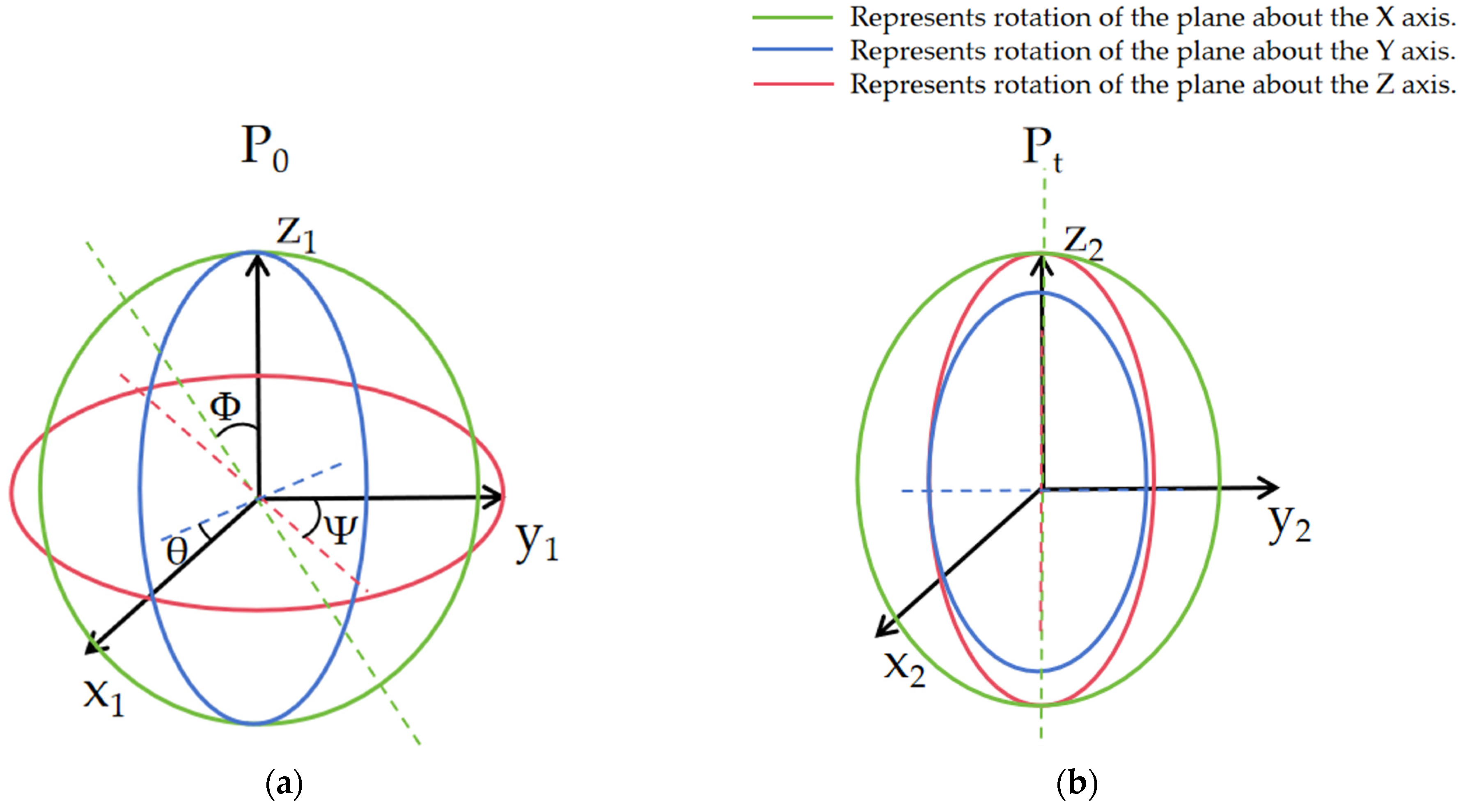
The spatial position of the vehicle fluctuates during operation due to variations in driving environments and road conditions. A vehicle in space has 6 degrees of freedom, as shown in Figure 1a, which include 3 translational degrees of freedom and 3 rotational degrees of freedom. These are commonly referred to as position and orientation information. The 3 rotational degrees of freedom are described using Euler angles. However, due to the occurrence of “gimbal lock” in Euler angles during mathematical calculations, as illustrated in Figure 1b, rotation matrices and quaternions are used to represent attitude information in SLAM.
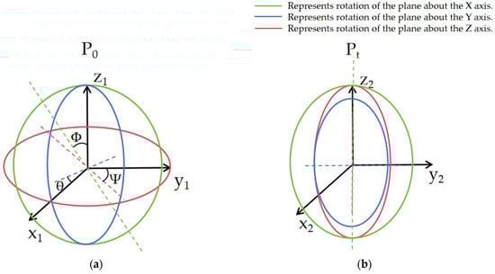
Figure 1.
Spatial pose map. (a) Six-degree of freedom diagram; (b) the phenomenon of “universal-joint locks”.
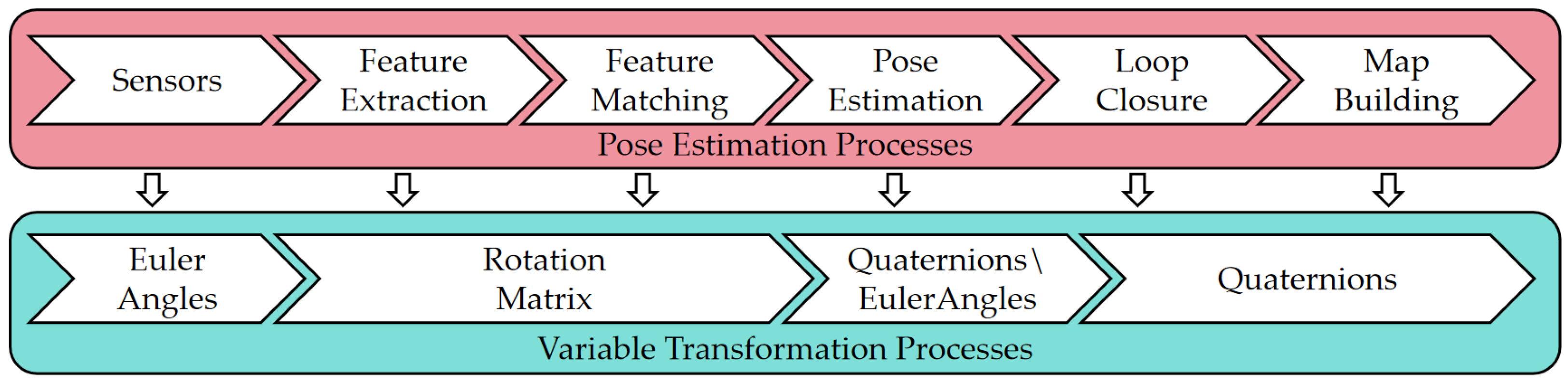
In summary, within SLAM algorithms, translational variables are represented using rectangular coordinates, while rotational variables are represented using Euler angles, rotation matrices, or quaternions. As discussed in the previous section, the state-of-the-art (SOTA) frameworks for 3D Lidar SLAM are ALOAM and LIO-SAM. Their pose estimation processes and rotational variable transformation processes are illustrated in Figure 2.
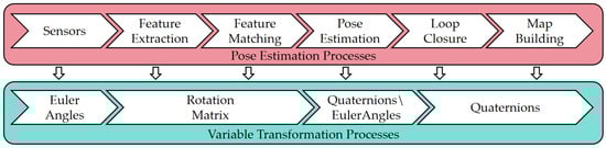
Figure 2.
The general transformation process of rotational variables in 3D Lidar SLAM.
Pose estimation involves converting between three representations: Euler angles, rotation matrices, and quaternions. In ALOAM, the rotational variables in the estimated pose are ultimately represented in the form of Euler angles. In LIO-SAM, due to the need to integrate with IMU odometry, the rotational variables in the estimated pose are ultimately represented in the form of quaternions. The relationships among these three types of rotational variables are as follows.
Euler angle can be expressed as
where is the roll angle; is the pitch angle; and is the yaw angle.
Quaternions can be expressed as
where is the scalar part; is the x-component vector part; is the y-component vector part; and is the z-component vector part.
The rotation matrix can be expressed as
where represents the elements of the matrix; is the row index; and is the column index.
The process of converting the rotation matrix to a quaternion is
The process of converting a quaternion to Euler angle is as follows:
For consistency with the standard evaluation tool EVO, we standardized the rotational variables in Lidar SLAM-based pose estimation to Euler angles.
2.1.2. Errors
The evaluation of localization anomalies in SLAM systems typically requires the introduction of two accuracy metrics: absolute pose error (APE) and relative pose error (RPE). These metrics were first defined in the TUM (Technical University of Munich) dataset [36]. APE and RPE are often used in combination to fully evaluate the performance of SLAM systems.
Absolute trajectory error (ATE) can directly reflect the positioning accuracy and map construction quality of the system in different scenarios. The absolute attitude error (APE) is calculated as the Euclidean distance between the system’s estimated attitude and the reference attitude, requiring that the timestamps between the system and the reference result be aligned to reflect the performance of the system.
The absolute trajectory error for the entire trajectory is defined as
where denotes Euclidean distance; is the pose of real track point; is the pose of the estimated locus point; and is the number of points in the trajectory.
For a single state, the absolute pose error of the estimated value and the real value satisfies
where represents the logarithm of the matrix; and represent the translation vector of the real pose and the estimated pose, respectively; and and represent the rotation vector of the real pose and the estimated pose, respectively.
For a single variable, the absolute error is:
where and represent the components of the real and estimated vectors in a certain direction, respectively; is the absolute value sign.
The absolute pose error (APE) has the advantage of being easy to compare. However, it is sensitive to the time of error and cannot directly observe and predict the trend of pose change. Therefore, in addition to APE, the RPE is also widely used, as it provides more time-related information.
The RPE measures the change in pose between two identical timestamps. It is typically computed as the Euclidean distance between the estimated relative pose and the reference relative pose, making it suitable for observing system drift during motion.
The relative trajectory error for the entire trajectory is defined as
where and denote the real pose and the estimated pose at the next time step, respectively.
For a single sub-trajectory, its relative pose error is
where and represent the translation vectors of the real pose and the estimated pose at the next time step, respectively; and correspond to the rotation vectors of the real pose and the estimated pose at the next time step, respectively.
For a single variable, the relative error is
where and signify variables in a particular direction for the real pose and the estimated pose, respectively.
2.2. Variable Correlation Analysis
As defined in Section 2.1, this study focuses on absolute and relative errors of translation and rotation variables, comprising 12 computational parameters in total. In order to explain the necessity of the study of each variable, the correlation analysis of variables is made.
The KITTI dataset was jointly created in 2012 by the Karlsruhe Institute of Technology (KIT) in Germany and the Toyota Institute of Technology in Chicago (TTI-Chicago) in the United States, and is one of the most commonly used computer vision algorithm evaluation dataset in automated driving scenarios [37]. The KITTI odometer section provides 11 sequences (00–10) for training. The sampling rate is 20 frames per second. The sequence scenarios and data packets are shown in Table 1.

Table 1.
KITTI odometer dataset scene situation and data volume.
Table 1 categorizes the KITTI dataset into the following types:
- Urban environment, complex roads: 00, 02, 08 (02 maximum data volume);
- Urban environment, short trajectory: 03, 05, 10 (05 maximum data volume);
- Urban environment, straight round-trip track: 06 (Straight-line loopback data in special scenarios);
- Urban environment, circular trajectory: 07, 09 (07 route is more structured, most researchers use this as their standard);
- Expressway: 01 (High speed scene radar failure is serious);
- Urban environment, straight track: 04 (The data is small and contained in other city scenarios).
We selected four representative trajectories (IDs: 02, 05, 06, 07) for analysis. We calculated positioning errors for four datasets by comparing pose estimates from the classical ALOAM framework against KITTI ground truth data, following Equations (1)–(16).
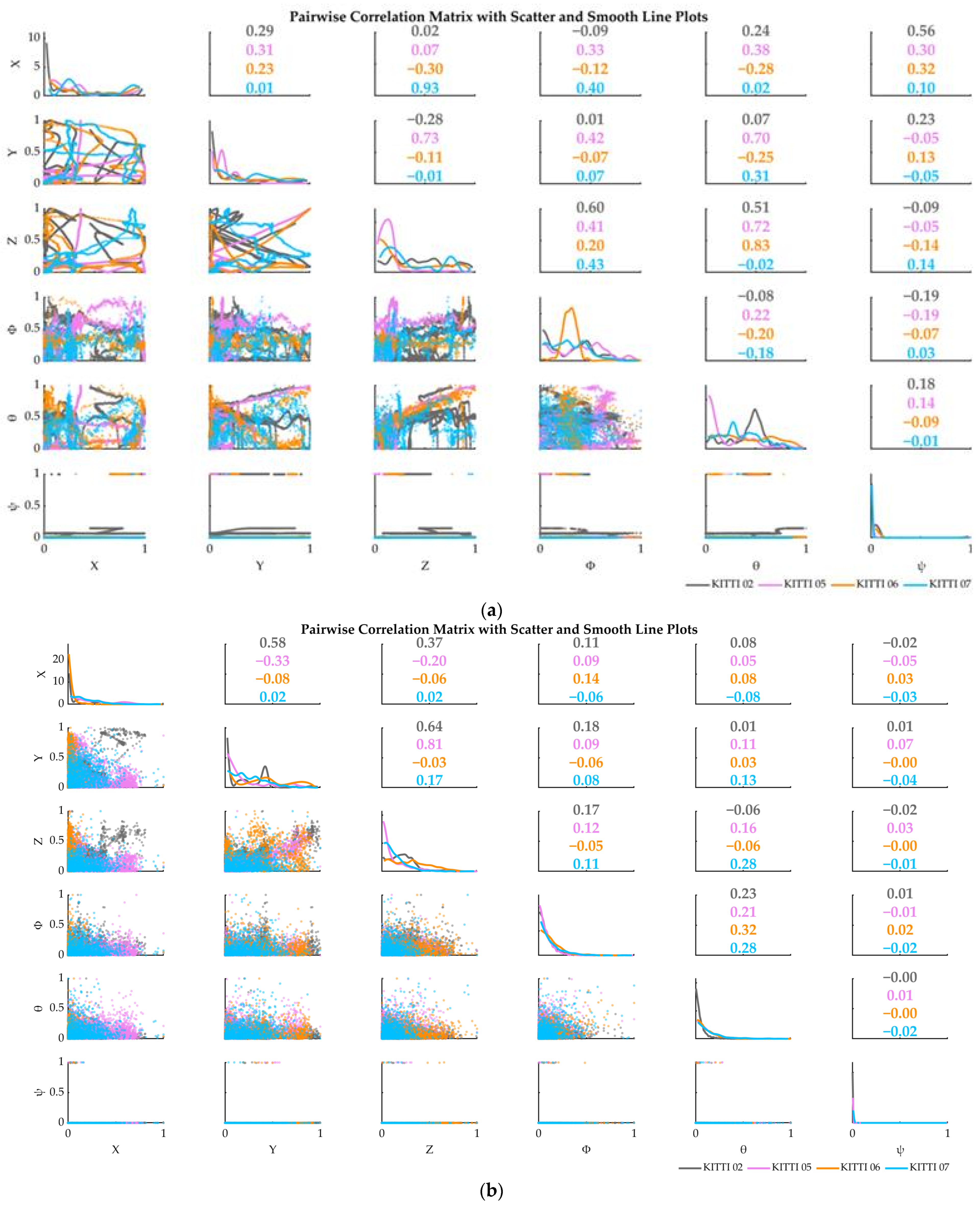
According to the calculation of Section 2.1, two errors of six variables can be obtained for each dataset, totaling twelve variables. In order to explain the necessity of the anomaly detection of each variable, the correlation coefficient of variables is calculated to explain the relationship between variables. The correlation analysis of pose variables was carried out using the calculation results of the above four datasets. The Pearson correlation coefficient is a statistical indicator of the degree of correlation between two variables, called the correlation coefficient. The correlation coefficient between two variables is defined as the quotient of covariance and standard deviation, as shown in Formula (17) [38].
where and are arbitrary variables; is the covariance between variable and variable ; is the standard deviations of the variable; and is the mathematical expectation.
Calculated according to the above formula, the correlation values and correlation scatterplots of APE data and RPE data of the respective variables in this research dataset are shown in Figure 3.
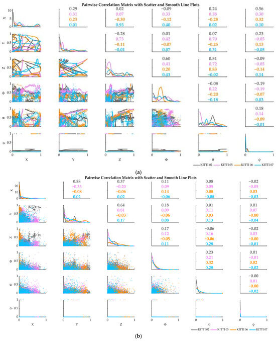
Figure 3.
Correlation analysis of variables. (a) Variable correlation analysis based on APE; (b) variable correlation analysis based on RPE.
When the correlation coefficient r < 0.5, the two variables show a moderate correlated. When the correlation coefficient r < 0.3, the two variables show a weak correlation [38]. As can be seen from Figure 3, most of the correlation coefficients of the 6 pose variables were in the weakly correlated range and distributed randomly among datasets.
Therefore, the scheme requires the real-time, independent and detailed detection of all variables in order to more directly observe abnormal changes in vehicle position and attitude.
3. Localization Anomaly Detection Algorithm
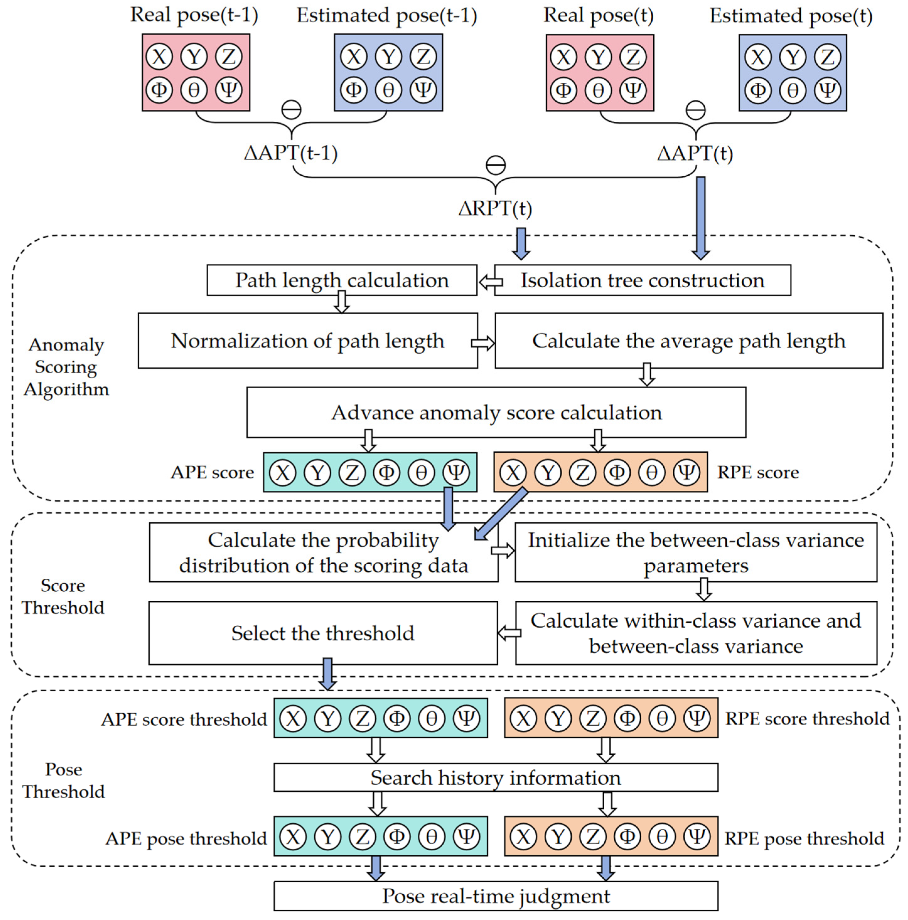
This part shows the specific algorithm calculation method of this paper. Figure 4 shows the flow chart of data processing.

Figure 4.
Algorithm detection procedure.
3.1. Isolation Forest Anomaly Scoring Algorithm
3.1.1. Classic Isolation Forest
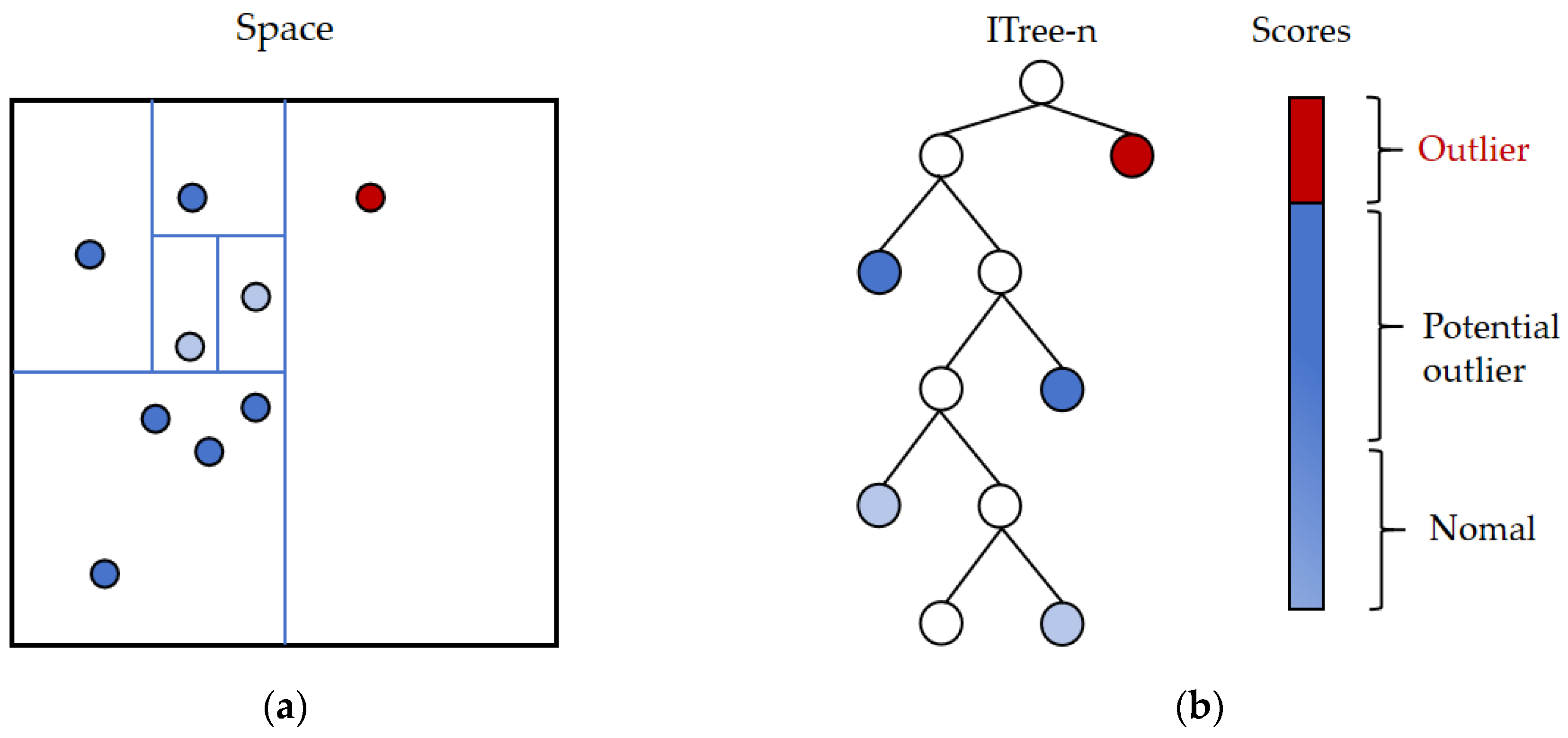
The isolation forest (iForest) employs a highly efficient strategy, utilizing a random hyperplane to split the data, generating two subspaces with each cut. This process continues with each subspace being further split by another random hyperplane, iterating until only one data point remains in each subspace [32]. Intuitively, dense clusters require many cuts to cease splitting, whereas sparse points quickly become isolated in a subspace. The iForest algorithm benefits from the concept of random forests; much like random forests consist of numerous decision trees, the iForest consists of numerous binary trees, known as isolation trees (iTrees). The construction of iTrees differs from that of decision trees and is simpler, involving a completely random process. The strategy of the algorithm is illustrated in Figure 5.
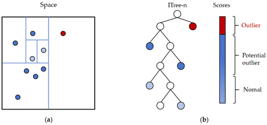
Figure 5.
IForest data processing procedure. (a) Data segmentation method; (b) isolated tree construction.
Iforest [32] can handle multiple variables at the same time, which is suitable for the six variables examined in this article. The iForest algorithm in this paper is described below.
- 1.
- Isolation tree construction.
Randomly select subsamples from the original data. Construct isolation trees (iTrees).
For each data point, the iForest recursively uses random features and random split values to partition the data, constructing a binary tree (iTree). Each partition generates two subspaces, and this process is repeated until each subspace contains only one data point.
- 2.
- Path length calculation.
The path length, , of a data point x is defined as the number of edges traversed from the root node to the leaf node in an iTree. This path length is indicative of how deeply a data point is isolated.
- 3.
- Calculate the average path length.
For a given data point , the average path length is computed by averaging the path lengths over all iTrees in the iForest.
- 4.
- Normalization of path length.
In the context of the iForest algorithm, represents the average path length of a data point . To make this average path length meaningful across different sample sizes, it needs to be normalized. This normalization is carried out using the reference value .
The reference value is derived from the harmonic number approximation and provides a baseline for comparison. This allows for the path length to be scaled appropriately, ensuring that the anomaly score is consistent regardless of the sample size. Without this normalization, the path length could be misleading due to variations in sample sizes.
The formula for is
where is the harmonic number, approximately (Euler’s constant) [32]. This helps in creating a standardized scoring mechanism for the algorithm.
- 5.
- Anomaly score calculation.
The anomaly score for a data point xx is calculated as
This score ranges between 0 and 1. Data points with scores closer to 1 are more likely to be anomalies. The closer the score is to zero, the more normal it is.
3.1.2. Advanced Scoring Formula
In the classic anomaly score calculation formula of the iForest, the anomaly score only considers the traversal path length, assuming that all nodes in the isolation trees have equal importance. This is a rather coarse assumption. Therefore, this paper introduces a path-weighted score to optimize the anomaly score calculation formula. The path-weighted score encodes the weight of each traversed node, and this weight is related to the structure of the isolation trees.
We redefined and rewrote it as . The formula quantifies the isolation difficulty of sample by weighting the weights of nodes on the summation path. This function is used to retrieve the path length of in tree , specifically expressed by the following formula:
where represents the weighted path length of the sample x in the isolated tree ; represents the path of a sample in a tree ; denotes the weight of node in tree . The more abnormal a point is, the shorter the corresponding path length is. The shorter the path length, the larger the weight, but the smaller the total weighted path.
The weight mentioned above is calculated using the following formula:
where represents the deep of samples contained in node of the isolation tree . The weight decays exponentially with the depth of the node, and the shallow node assigns a higher weight to reflect the rapid isolation of the anomaly at the shallow layer. The more abnormal the point, the shallower the number of layers and the greater the weight.
Finally, the formula for the proposed anomaly score is as follows:
By optimizing the anomaly score formula, we assigned higher weights to anomalous samples (those separated earlier), while reducing the weights for normal samples. These weights are determined based on the structure of the isolation tree itself, specifically the number of samples contained in node . The improved scoring formula exhibits greater sensitivity to local anomalies.
In summary, the more abnormal the point is and the shorter the path length is, the closer the S value is to 1. As can be seen from Section 3.1.1: Data points with scores closer to 1 are more likely to be anomalies.
3.2. Adaptive Score Thresholding Using the Otsu Method
To make the algorithm proposed in this paper closer to a completely unsupervised method, the Otsu thresholding method (Otsu) algorithm is adopted to adaptively set the threshold for anomaly scores [39]. In the classic iForest algorithm, the threshold for anomaly scores is manually set, usually based on the contour of the anomaly scores, which is a rather vague method. The threshold has a great influence on the accuracy of anomaly detection, so the selection of scoring threshold is particularly important. Therefore, this paper utilizes Otsu’s method to precisely determine the threshold for anomaly scores.
Otsu’s method is a technique for determining the binarization threshold of an image. It divides the original samples into two classes and adaptively sets the threshold based on the principle of maximizing inter-class variance. The traditional OTSU method requires setting the sample size, and the experiment is relatively subjective. By adopting an adaptive approach, the results become independent of the scale of the input data. In terms of reliability, the optimization model avoids the randomness of artificial parameter adjustment and improves the repeatability of system results. Adapting to the distribution of different data can enhance the generalization ability of the system. An adaptive mechanism is introduced to enhance the robustness of the dynamic distribution of the system. The adaptive mechanism supports unsupervised learning and improves the reliability of the model in practical applications.
The specific formula and calculation steps are as follows:
- 1.
- Calculate the probability distribution of the scoring data.
Adaptive selection of histogram sizes: Dynamically set the number of bin of the histogram based on the initial input size of the score dataset, using the square root of the sample size rounded to the nearest integer (minimum 10):
Determine the width of each bin () based on the data range and the number of bins :
where range represents the difference between the maximum and minimum values of the scoring dataset.
Count the number of data points in each bin and calculate the probability distribution for each bin:
where represents the number of data points in bin ; is the total number of data points in the dataset variance parameters.
- 2.
- Initialize the between-class variance parameters.
Calculate the overall mean :
where represents all possible thresholds and is determined based on each bin boundry in the histogram.
- 3.
- Iterate over each possible threshold and calculate the within-class variance and between-class variance.
Initialize the weights, means, and variances for Class 1 (data below the threshold) and Class 2 (data above the threshold):
Calculate the between-class variance :
- 4.
- Select the threshold corresponding to the maximum between-class variance.
Iterate over each possible threshold and calculate the within-class variance and between-class variance for each . Choose the threshold that maximizes the between-class variance:
- 5.
- Output the final threshold.
Calculate and output the final optimal threshold for data classification.
4. Experiments and Results Analysis
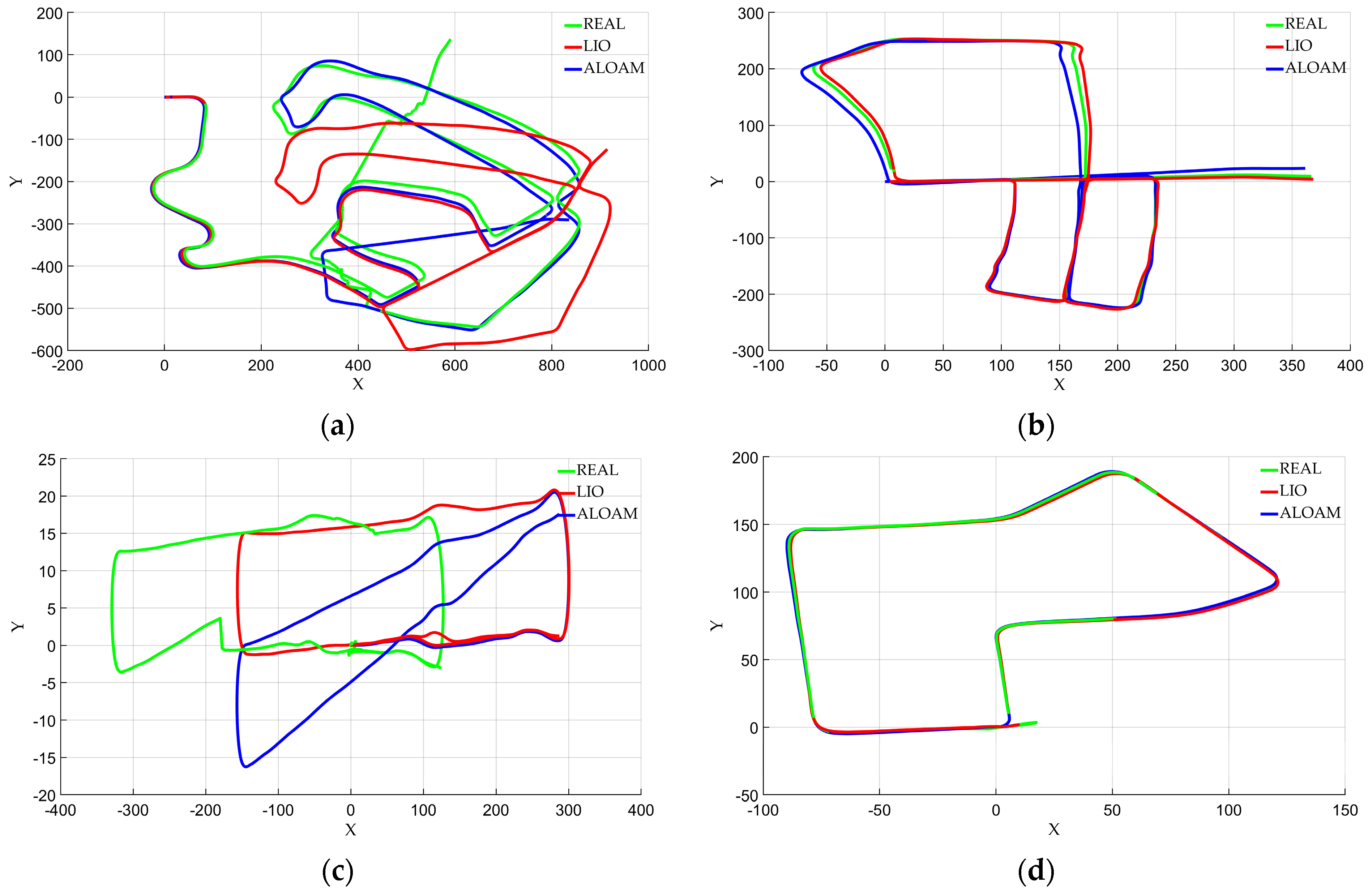
This section describes anomaly detection in positioning of KITTI dataset based on the above analysis. In order to prove the universality of this algorithm to anomaly location data detection, experiments were carried out using the ALOAM framework and LIO-SAM framework. Both frameworks use uniform external parameters and do not make individual adjustments to each dataset, so there are different positioning anomalies (drift or even loss). The result path of the dataset is shown in Figure 6. All the experiments in this paper were conducted based on the path conditions in the figure. As can be seen from the figure, the experimental data are irregular time-series data changing with time.
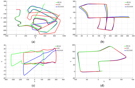
Figure 6.
KITTI dataset real path and Lidar SLAM result path: (a) 02 sequence; (b) 05 sequence; (c) 06 sequence; (d) 07 sequence.
4.1. Evaluation Metrics
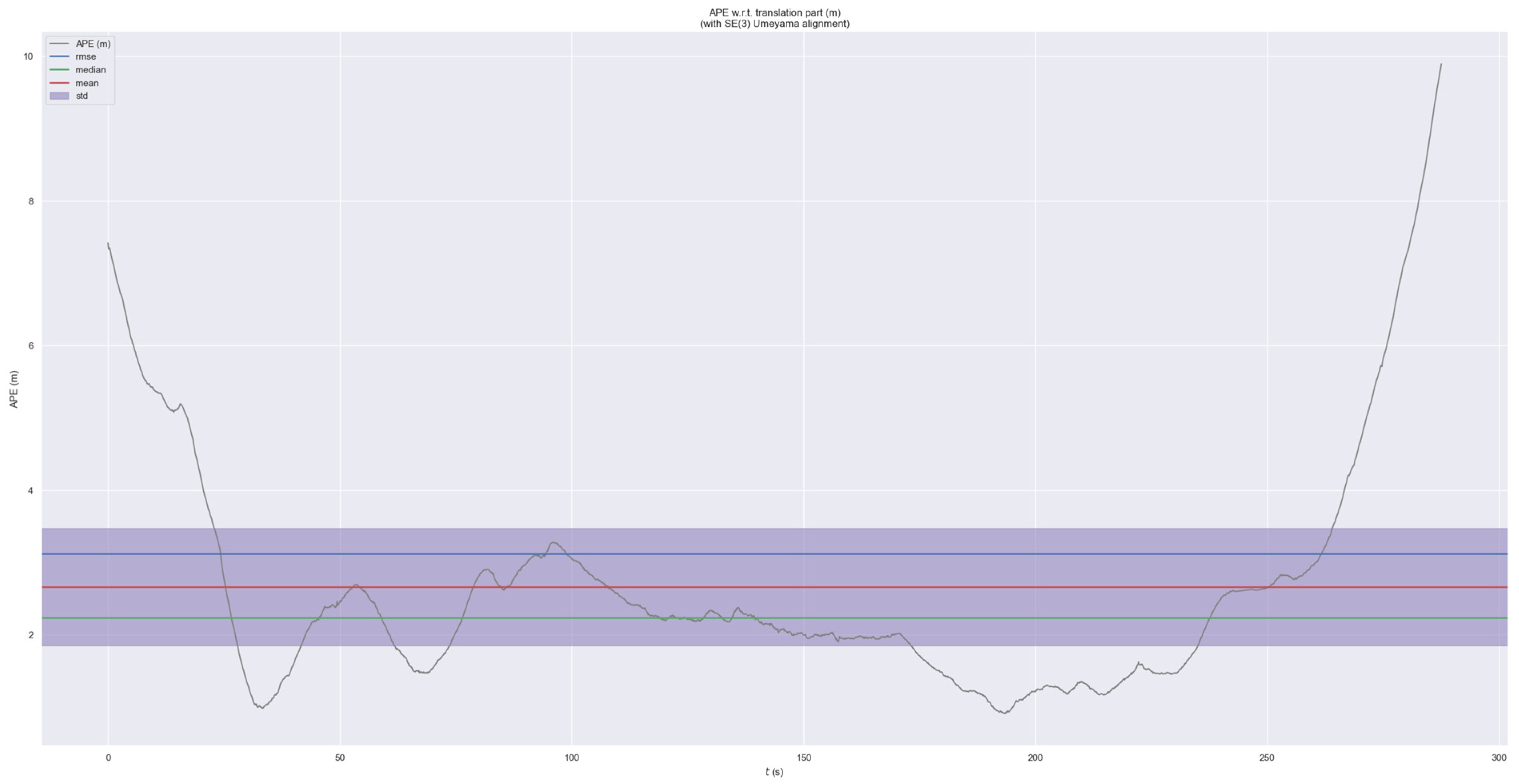
EVO is a widely used tool for SLAM evaluation. It assesses the accuracy of SLAM algorithms by comparing the estimated trajectory obtained after the vehicle’s operation with the ground truth trajectory. Engineers typically use EVO for parameter threshold adjustment, as shown in Figure 7. The error-related curves provide the following reference data: root mean square error (RMSE), which measures the square root of the average squared errors; median error; mean error; standard deviation (Std), which describes the dispersion of the errors [8].
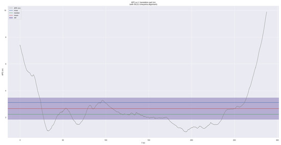
Figure 7.
Sequence APE in EVO visualization.
The formula for calculating RMSE and Std is as follows.
The Mean error:
where is the error value of the point; is the number of points.
RMSE:
Error standard deviation range Std:
These are the most common methods for determining outlier thresholds. If the threshold is set too high, the system reliability will be reduced, and if the threshold is set too small, the system robustness will be poor. There is a certain game relationship between the sensitivity of the system and false positives, but considering the high safety of the intelligent driving system, we give priority to the sensitivity of the algorithm. Based on this, the median line (mean value-) of the Std region is used as the threshold reference object in this paper. We compare the absolute and relative error thresholds obtained in this paper with the reference values () derived from the above evaluation criteria.
4.2. Hardware Configuration and Software Environment
- Hardware Configuration:
Processor: Intel Core i7-12700H; Graphics Card: NVIDIA GeForce RTX 3060 6 GB.
- Software Environment:
ROS1; C++14; OpenCV (4.2.0); Ceres Solver (1.14); PCL (1.10.0); Eigen (3.3); Gtsam (4.0.2); GeographicLib (1.50); Catkin (0.7.17); Yaml-cpp (0.5.3).
4.3. Results and Analysis of the ALOAM Framework
In this section, we analyze four datasets that broadly cover the most diverse outdoor scenarios in the KITTI dataset. The external parameters of ALOAM framework did not change with the change of dataset, so there are different anomalies in the trajectory results compared with the true values in different datasets. The visualization of detection results shows the detection performance and environment generalization ability of our algorithm. The effectiveness and accuracy of the algorithm are illustrated by comparing it with reference data. Finally, the superiority of the optimization algorithm is verified by comparative experiments.
4.3.1. Result Visualization
The traditional iForest algorithm uses 256 samples for scoring [32], while the EVO (1.31.1) software uses the full path for calculating reference values. It is unfair to compare the sampling threshold of the algorithm with that of the full path, so this paper sets the number of samples uniformly to 300 for the calculation involved.
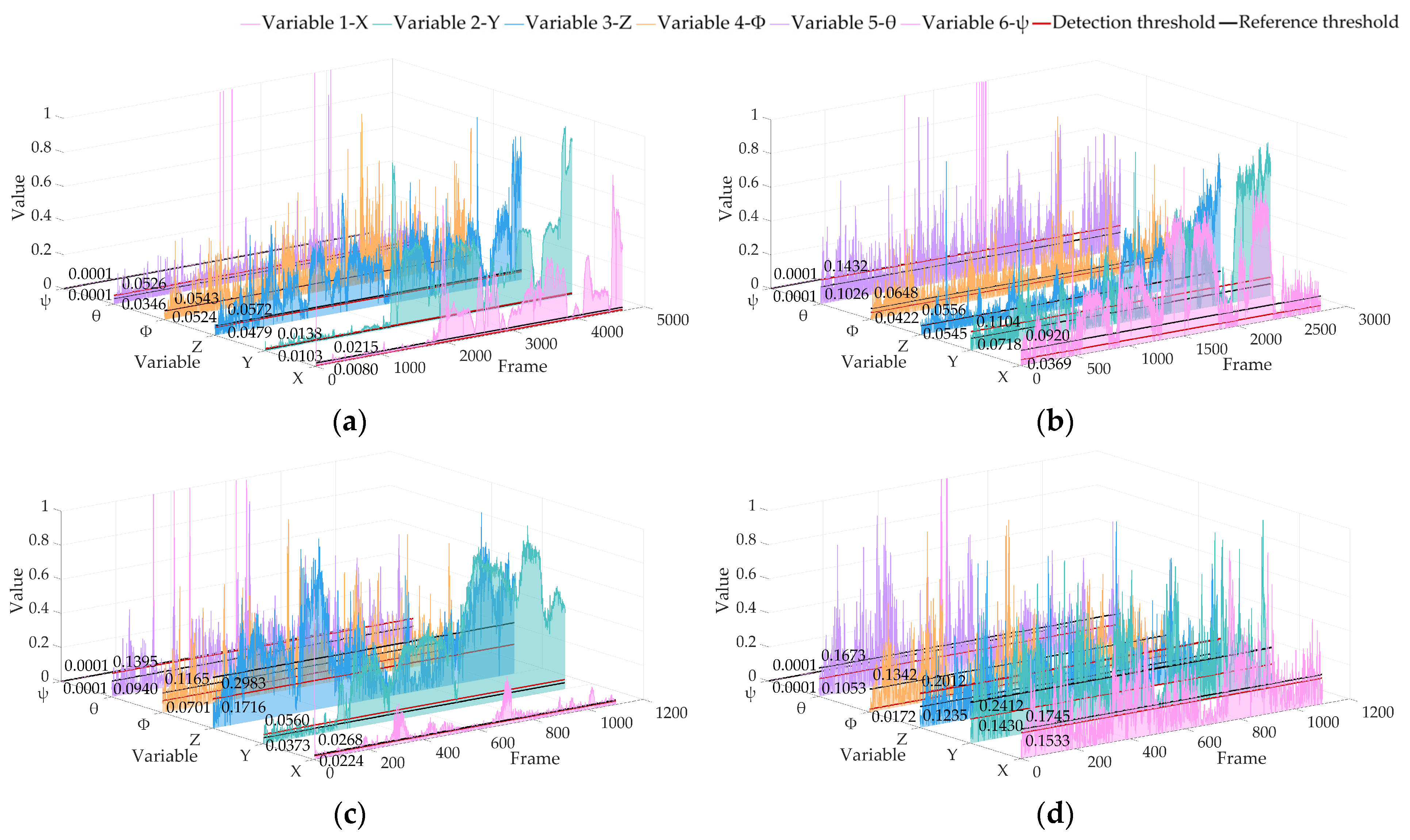
Because of the different values of variables, the visualization of all variables is normalized in this paper. Figure 8 shows the APE results of datasets 02, 05, 06 and 07 obtained by the real-time operation of the algorithm in this paper, showing the positioning anomaly detection results of six pose variables.
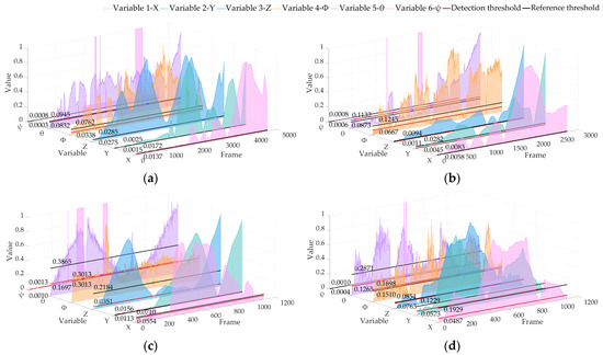
Figure 8.
Locating abnormal APE detection results based on the KITTI dataset of ALOAM. The red line is the detection threshold, and the black line is the reference threshold: (a) 02 sequence; (b) 05 sequence; (c) 06 sequence; (d) 07 sequence.
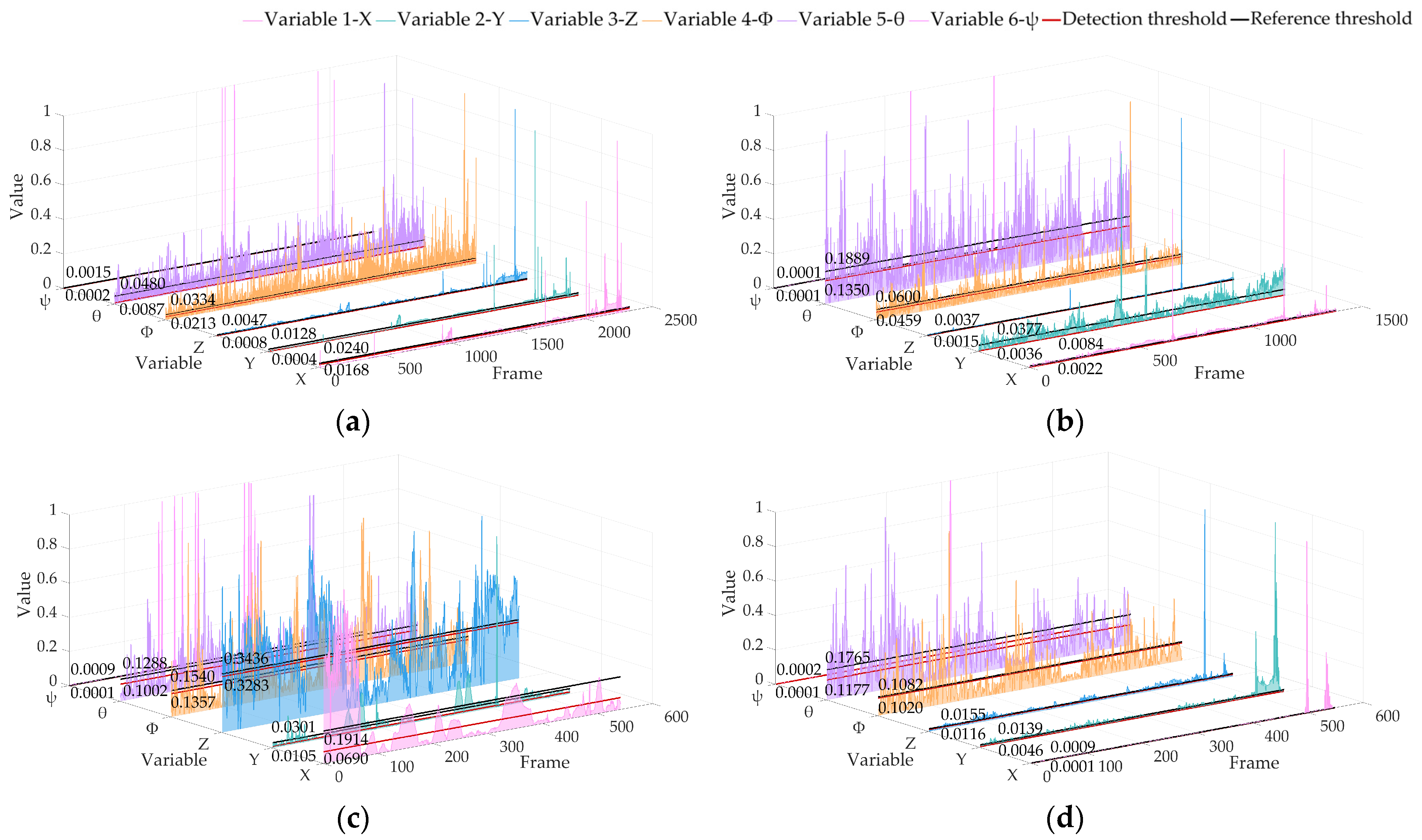
Figure 9 shows the RPE results of datasets 02, 05, 06 and 07 obtained by the real-time operation of the algorithm in this paper, showing the positioning anomaly detection results of six pose variables.
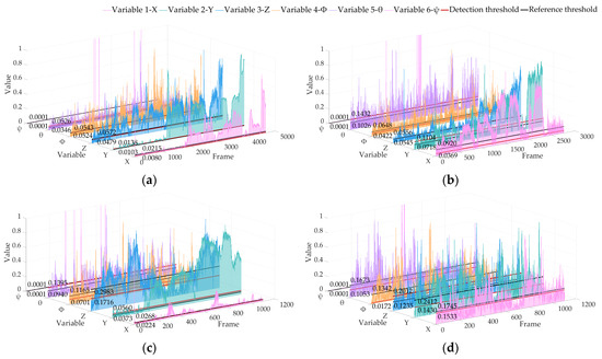
Figure 9.
Locating abnormal RPE detection results based on the KITTI dataset of ALOAM. The red line is the detection threshold, and the black line is the reference threshold: (a) 02 sequence; (b) 05 sequence; (c) 06 sequence; (d) 07 sequence.
Algorithm running time is as follows:
- Max time: 0.03999 s;
- Min time: 0.009402 s;
- Mean time: 0.020577 s.
As can be seen from Table 1, the data rate is 20 frames/s, that is, 0.05 s/frame. The running time of the algorithm is less than the data rate and meets the real-time standard.
It can be seen from the results that the threshold calculated by our algorithm in real time is better than the trajectory posterior threshold under the premise of keeping the sampling fair. The above analysis shows that our algorithm has high sensitivity to variable changes and can be used to detect the anomaly of vehicle pose changes in real time. The results of APE and RPE show that our algorithm can accurately identify sudden changes and analyze changing trends without a lot of prior training for the algorithm.
4.3.2. Result Evaluation and Algorithm Comparison
Formulas (33)–(35) were used to obtain reference values and reference intervals. The proposed algorithm was compared with IF-OTSU, IF, K-means and SVM algorithms. The relevant algorithm sampled the same number as previously set: 300. The datasets used in this study were unlabeled, and the authors did not subjectively evaluate the datasets due to the subjective nature of the assessment. Generally speaking, the smaller the threshold, the more timely and effective system jitter can be detected. Therefore, this paper only compared the threshold values detected with those of other methods.
There are many variables in this paper, so the translation variable and the rotation variable were compared comprehensively. The calculation method is as follows:
The results of data evaluation and algorithm comparison are summarized in Table 2, where the unit for parameter T is meters (m) and for parameter R is radians (rad). To account for the stochastic nature of the algorithm’s random operators, the values presented in the table represent the average outcomes derived from five independent experimental trials for each dataset.
Table 2.
Evaluation and algorithm comparison of ALOAM.
From the above results, it can be seen that our algorithm can accurately identify abnormal data in real time without supervision, and do not need to be trained on specific datasets. The model in this paper can detect each variable of pose at the same time, and comprehensively cover the recognition of anomalies.
The results are within the Std range of the EVO calculation and close to the mean results. The comparison with ablative method also shows the superiority of this algorithm. K-means, relying on distance-based assumptions, is sensitive to non-spherical clusters and outliers, which can result in disruptions caused by anomalies (e.g., shifts in centroids). Moreover, the curse of dimensionality diminishes the discriminative power of Euclidean distance in high-dimensional spaces, adversely affecting clustering performance. Similarly, SVMs exhibited high computational complexity and were sensitive to parameter tuning, making hyperparameter optimization challenging. In high-dimensional spaces, data sparsity may hinder the hyperplane’s ability to effectively separate normal and anomalous regions [35]. Based on the above analysis and the results presented in Table 2, our proposed algorithm demonstrated superior sensitivity and accuracy in anomaly detection compared to SOTA methods, effectively addressing the limitations of conventional approaches while maintaining computational efficiency.
4.4. Results and Analysis of the LIO-SAM Framework
In order to show the universality of this algorithm, this part discusses the anomaly detection of the pose estimation results of LIO-SAM system. LIO-SAM is a fusion SLAM system of radar and IMU. The datasets and algorithm sampling interval preparation are the same as in Section 4.3.
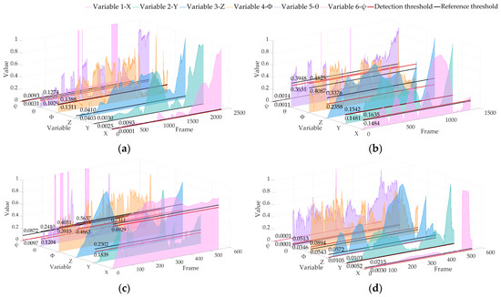
Figure 10.
Locating abnormal APE detection results based on the KITTI dataset of LIO-SAM. The red line is the detection threshold, and the black line is the reference threshold: (a) 02 sequence; (b) 05 sequence; (c) 06 sequence; (d) 07 sequence.
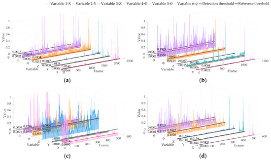
Figure 11.
Locating abnormal RPE detection results based on the KITTI dataset of LIO-SAM. The red line is the detection threshold, and the black line is the reference threshold: (a) 02 sequence; (b) 05 sequence; (c) 06 sequence; (d) 07 sequence.
The algorithm running time is as follows:
- Max time: 0.027024 s;
- Min time: 0.0094382 s;
- Mean time: 0.017034467 s.
It can be seen from Figure 10 and Figure 11 that our algorithm can also calculate the threshold in real time in LIO-SAM and is better than the trajectory posterior threshold. The above analysis shows that the algorithm has a high sensitivity to the variable changes of the pose estimation results, and can be used to detect the vehicle attitude changes in real time. The results show that the proposed algorithm is not limited by the specific framework, and can monitor and analyze the variables comprehensively.
The results of data evaluation and algorithm comparison are summarized in Table 3, where the unit for parameter T is meters (m) and for parameter R is radians (rad). To account for the stochastic nature of the algorithm’s random operators, the values pre-sented in the table represent the average outcomes derived from five independent ex-perimental trials for each dataset.
Table 3.
Evaluation and algorithm comparison of LIO-SAM.
Table 3 shows that, although under a different framework, our results are still within the Std range calculated by EVO and close to the value of Mean. The comparison with the ablation algorithm also shows the superiority of the proposed algorithm. Compared with the SOTA algorithm, this algorithm is also more sensitive to anomalies.
As can be seen from the above results, our algorithm can be migrated to other Lidar SLAM to accurately identify abnormal data in real time without supervision.
In summary, from the detection effects of different systems in the above rich datasets, it can be concluded that our algorithm can adapt to different scene environments. As long as the output form of the result estimation pose of laser slam system is known, the proposed method can be used to detect the positioning change. Under the premise of unknown whether there are dynamic obstacles and environmental changes in the vehicle operation scene, the positioning changes caused by the environment and the sensor’s own noise can also be sensitively detected.
5. Discussion and Conclusions
The purpose of SLAM algorithms is to construct high-precision maps and localization frameworks in real time [40]. SLAM occupies a crucial position in the field of smart driving and is an indispensable component of perception algorithms. Lidar is considered as the core sensor in the strong perception scheme [41]. However, due to the noise from the vehicle’s sensors and the complex environmental noise, achieving accurate SLAM in dynamic environments is extremely challenging [1,2]. Current research directions aim for extreme accuracy, but due to the high complexity of SLAM systems, it is difficult to develop an autonomous system that can adapt to all environments without manual intervention. Errors in SLAM systems directly contribute to accumulated errors or even failures in downstream tasks, severely impacting the accuracy of intelligent driving systems [3]. Addressing these challenges requires innovative methods that can accurately monitor system changes in real-time, independent of the environment.
In this work, we propose an unsupervised isolation forest detection method to tackle the aforementioned challenges. To enhance the model’s sensitivity to anomalies and improve the scoring system, we adopted a path-weighted method for scoring each value. To achieve a near-total autonomy of the model, we utilized adaptive OTSU for scoring classification, which is not constrained by sample size. The model self-adjusts the sampling window size to handle scoring classification. Experiments conducted on the KITTI dataset and various Lidar SLAM systems demonstrated the real-time performance and effectiveness of our work. Compared to EVO’s trajectory posterior analysis tool, our model showed higher accuracy, validating the superiority of our real-time detection method. Notably, when compared with similar algorithms and ablation algorithms, our approach still displayed significant advantages.
Future research and expansion can be considered in the following ways. In terms of sensors, this paper only studies lasers. Further combining with visual SLAM to estimate pose results, our method can be applied to multi-sensor fusion SLAM localization detection. In terms of coordinate calibration, this paper needs to understand the manual alignment of coordinate axes with different frames. The automatic calibration of different SLAM system variables can also be developed, which will allow for algorithms to autonomously switch recognition in multimodal SLAM. In terms of algorithm evolution, back-end optimization and relocation can be considered. Thus, the relationship between variables and driving trajectory or operating conditions can be further analyzed, and specific variables can be independently corrected, thereby improving the accuracy and safety of the entire system. In terms of fault condition analysis, scene or driving status labels can be set for multiple data set scenarios. This will further analyze and locate the source of the fault, thereby reducing the false positives of the algorithm and improving and enhancing the performance of the slam system.
In summary, this paper presents an innovative detection model for the stability and safety of Lidar SLAM systems. The model meets the real-time requirements of SLAM systems while achieving unsupervised pose data detection in various environments. By leveraging the isolation forest algorithm and adaptive OTSU classification method, it demonstrates the potential for extensible research in the field of SLAM with a focus on engineering safety. Future work should continue developing general models, gradually reducing the reliance of SLAM systems on extensive external parameters, thus contributing to the robustness of intelligent driving.
Author Contributions
Conceptualization, G.G. and P.W.; methodology, G.G. and P.W.; software, P.W.; validation, P.W., G.G. and H.W.; formal analysis, P.W.; investigation, P.W. and H.W.; resources, G.G.; data curation, P.W.; writing—original draft preparation, P.W.; writing—review and editing, G.G., P.W. and L.S.; visualization, P.W.; supervision, G.G.; project administration, G.G. and L.S.; funding acquisition, G.G. All authors have read and agreed to the published version of the manuscript.
Funding
This research was supported by the key research and development program of Jiangsu Province, China: R&D of Integrated Control of Intelligent Transportation and Chassis Electric Integration (BE2019010).
Data Availability Statement
Publicly available datasets were used in this study. The KITTI dataset can be found at https://www.cvlibs.net/datasets/kitti/eval_odometry.php (accessed on 17 June 2023).
Conflicts of Interest
The authors declare no conflicts of interest.
Abbreviations
The following abbreviations are used in this manuscript:
| ALOAM | Advanced Lidar odometry and mapping |
| APE | Absolute pose error |
| ATE | Absolute trajectory error |
| DBSCAN | Density-based spatial clustering of applications with noise |
| EVO | Evaluation of odometry |
| Gtsam | Georgia Tech Smoothing and Mapping |
| IF | Isolation forest |
| iForest | Isolation forest |
| iTree | Isolation tree |
| KITTI | Karlsruhe Institute of Technology and Toyota Technological Institute |
| LIO-SAM | LiDAR inertial odometry via smoothing and mapping |
| LOF | Local outlier factor |
| OTSU | Otsu’s method (thresholding) |
| OpenCV | Open-Source Computer Vision Library |
| PCA | Principal component analysis |
| PCL | Point Cloud Library |
| PTE | Pose tracking error |
| REMS | Recursive environmental monitoring system |
| ROS1 | Robot Operating System 1 |
| RPE | Relative pose error |
| RTX | Ray Tracing Texel |
| SLAM | Simultaneous localization and mapping |
| SOTA | State Of the art |
| Std | Standard deviation |
| SVM | Support vector machine |
| TUM | Technical University of Munich |
References
- Singandhupe, A.; La, H.M. A Review of SLAM Techniques and Security in Autonomous Driving. In Proceedings of the 2019 Third IEEE International Conference on Robotic Computing (IRC), Naples, Italy, 25–27 February 2019; pp. 602–607. [Google Scholar]
- Zheng, S.; Wang, J.; Rizos, C.; Ding, W.; El-Mowafy, A. Simultaneous Localization and Mapping (SLAM) for Autonomous Driving: Concept and Analysis. Remote Sens. 2023, 15, 1156. [Google Scholar] [CrossRef]
- Cadena, C.; Carlone, L.; Carrillo, H.; Latif, Y.; Scaramuzza, D.; Neira, J.; Reid, I.; Leonard, J.J. Past, Present, and Future of Simultaneous Localization and Mapping: Toward the Robust-Perception Age. IEEE Trans. Robot. 2016, 32, 1309–1332. [Google Scholar] [CrossRef]
- Yong, L.; Jiexin, A.; Na, H.; Yanbo, L.; Zhenyu, H.; Zishan, C.; Yaping, Q. A Review of Simultaneous Localization and Mapping Algorithms Based on Lidar. World Electr. Veh. J. 2025, 16, 56. [Google Scholar] [CrossRef]
- Zhang, J.; Singh, S. LOAM: Lidar Odometry and Mapping in Real-Time. In Proceedings of the Robotics: Science and Systems Foundation, Berkeley, CA, USA, 12–16 July 2014. [Google Scholar]
- Shan, T.; Englot, B.; Meyers, D.; Wang, W.; Ratti, C.; Rus, D. LIO-SAM: Tightly-Coupled Lidar Inertial Odometry via Smoothing and Mapping. In Proceedings of the 2020 IEEE/RSJ International Conference on Intelligent Robots and Systems (IROS), Las Vegas, NV, USA, 25–29 October 2020; pp. 5135–5142. [Google Scholar]
- Huang, L. Review on Lidar SLAM Techniques. In Proceedings of the 2021 International Conference on Signal Processing and Machine Learning (CONF-SPML), Beijing, China, 14 November 2021; pp. 163–168. [Google Scholar]
- Evo: Python Package for the Evaluation of Odometry and SLAM. Available online: https://github.com/MichaelGrupp/evo (accessed on 19 July 2023).
- Gelfand, N.; Ikemoto, L.; Rusinkiewicz, S.; Levoy, M. Geometrically Stable Sampling for the ICP Algorithm. In Proceedings of the Fourth International Conference on 3-D Digital Imaging and Modeling, Banff, AB, Canada, 6–10 October 2003; pp. 260–267. [Google Scholar]
- Kwok, T.H.; Tang, K. Improvements to the Iterative Closest Point Algorithm for Shape Registration in Manufacturing. J. Manuf. Sci. Eng. 2015, 138, 011014. [Google Scholar] [CrossRef]
- Zhen, W.; Scherer, S. Estimating the Localizability in Tunnel-like Environments Using Lidar and UWB. In Proceedings of the 2019 International Conference on Robotics and Automation (ICRA), Montreal, QC, Canada, 20–24 May 2019; pp. 4903–4908. [Google Scholar]
- Rong, Z.; Michael, N. Detection and Prediction of Near-Term State Estimation Degradation via Online Nonlinear Observability Analysis. In Proceedings of the 2016 IEEE International Symposium on Safety, Security, and Rescue Robotics (SSRR), Kobe, Japan, 7–11 October 2016; pp. 28–33. [Google Scholar]
- Cho, H.; Yeon, S.; Choi, H.; Doh, N. Detection and Compensation of Degeneracy Cases for IMU-Kinect Integrated Continuous SLAM with Plane Features. Sensors 2018, 18, 935. [Google Scholar] [CrossRef] [PubMed]
- Tagliabue, A.; Tordesillas, J.; Cai, X.; Santamaria-Navarro, A.; How, J.P.; Carlone, L. LION: Lidar-Inertial Observability-Aware Navigator for Vision-Denied Environments. In Proceedings of the Experimental Robotics The 17th International Symposium (ISER 2020), La Valletta, Malta, 15–18 November 2021. [Google Scholar]
- Liu, Y.; Wang, J.; Huang, Y. A Localizability Estimation Method for Mobile Robots Based on 3D Point Cloud Feature. In Proceedings of the 2021 IEEE International Conference on Real-Time Computing and Robotics (RCAR), Xining, China, 15–19 July 2021; pp. 1035–1041. [Google Scholar]
- Dong, L.; Chen, W.; Wang, J. Efficient Feature Extraction and Localizability Based Matching for Lidar SLAM. In Proceedings of the 2021 IEEE International Conference on Robotics and Biomimetics (ROBIO), Sanya, China, 27–31 December 2021; pp. 820–825. [Google Scholar]
- Nashed, S.B.; Jin Park, J.; Webster, R.; Durham, J.W. Robust Rank Deficient SLAM. In Proceedings of the 2021 IEEE/RSJ International Conference on Intelligent Robots and Systems (IROS), Prague, Czech Republic, 27 September 2021–1 October 2021; pp. 6603–6608. [Google Scholar]
- Rodríguez-Arévalo, M.L.; Neira, J.; Castellanos, J.A. On the Importance of Uncertainty Representation in Active SLAM. IEEE Trans. Robot. 2018, 34, 829–834. [Google Scholar]
- Zhang, J.; Kaess, M.; Singh, S. On Degeneracy of Optimization-Based State Estimation Problems. In Proceedings of the 2016 IEEE International Conference on Robotics and Automation (ICRA), Stockholm, Sweden, 16–21 May 2016; pp. 809–816. [Google Scholar]
- Jiao, J.; Ye, H.; Zhu, Y.; Liu, M. Robust Odometry and Mapping for Multi-Lidar Systems with Online Extrinsic Calibration. IEEE Trans. Robot. 2022, 38, 351–371. [Google Scholar] [CrossRef]
- Westman, E.; Kaess, M. Degeneracy-Aware Imaging Sonar Simultaneous Localization and Mapping. IEEE J. Ocean. Eng. 2020, 45, 1280–1294. [Google Scholar] [CrossRef]
- Ren, R.; Fu, H.; Xue, H.; Sun, Z.; Ding, K.; Wang, P. Towards a Fully Automated 3D Reconstruction System Based on Lidar and GNSS in Challenging Scenarios. Remote Sens. 2021, 13, 1981. [Google Scholar] [CrossRef]
- Zhou, H.; Yao, Z.; Lu, M. Lidar/UWB Fusion Based SLAM With Anti-Degeneration Capability. IEEE Trans. Veh. Technol. 2021, 70, 820–830. [Google Scholar]
- Nobili, S.; Tinchev, G.; Fallon, M. Predicting Alignment Risk to Prevent Localization Failure. In Proceedings of the 2018 IEEE International Conference on Robotics and Automation (ICRA), Brisbane, Australia, 21–25 May 2018; pp. 1003–1010. [Google Scholar]
- Chen, X.; Läbe, T.; Milioto, A. OverlapNet: A siamese network for computing LiDAR scan similarity with applications to loop closing and localization. Auton. Robot. 2022, 46, 61–81. [Google Scholar]
- Gao, Y.; Wang, S.Q.; Li, J.H.; Hu, M.Q.; Xia, H.Y.; Hu, H.; Wang, L.J. A Prediction Method of Localizability Based on Deep Learning. IEEE Access 2020, 8, 110103–110115. [Google Scholar] [CrossRef]
- Dani, M.C.; Jollois, F.X.; Nadif, M.; Freixo, C. Adaptive Threshold for Anomaly Detection Using Time Series Segmentation. In Proceedings of the Neural Information Processing: 22nd International Conference (ICONIP 2015), Istanbul, Turkey, 9–12 November 2015. [Google Scholar]
- Huang, T.; Zhu, Y.; Zhang, Q.; Zhu, Y.; Wang, D.; Qiu, M.; Liu, L. An LOF-Based Adaptive Anomaly Detection Scheme for Cloud Computing. In Proceedings of the 2013 IEEE 37th Annual Computer Software and Applications Conference Workshops, Kyoto, Japan, 22–26 July 2013; pp. 206–211. [Google Scholar]
- XIaoyu, L.; Xiao, G.; Zhaosheng, Z.; Qiping, C.; Zhenpo, W. Fault Diagnosis and Detection for Battery System in Real-World Electric Vehicles Based on Long-Term Feature Outlier Analysis. IEEE Trans. Transp. Electrif. 2024, 10, 1668–1679. [Google Scholar]
- Ehsan, N.; Arash, A. Toward Detecting Cyberattacks Targeting Modern Power Grids: A Deep Learning Framework. In Proceedings of the 2022 IEEE World AI IoT Congress (AIIoT), Seattle, WA, USA, 6–9 June 2022; pp. 357–363. [Google Scholar]
- Ehsan, N.; Arash, A. Detection of False Data Injection Cyberattacks: Experimental Validation on a Lab-scale Microgrid. In Proceedings of the 2022 IEEE Green Energy and Smart System Systems (IGESSC), Seattle, WA, USA, 13 July 2022; pp. 1–6. [Google Scholar]
- Liu, F.T.; Ting, K.M.; Zhou, Z.H. Isolation Forest. In Proceedings of the Eighth IEEE International Conference on Data Mining, Pisa, Italy, 15 December 2008; pp. 413–422. [Google Scholar]
- Novakov, S.; Lung, C.-H.; Lambadaris, I.; Seddigh, N. Studies in Applying PCA and Wavelet Algorithms for Network Traffic Anomaly Detection. In Proceedings of the 2013 IEEE 14th International Conference on High Performance Switching and Routing (HPSR), Vienna, Austria, 3–6 July 2013; pp. 185–190. [Google Scholar]
- Chen, Y.; Chen, L.; Huang, C.; Lu, Y.; Wang, C. A dynamic tire model based on HPSO-SVM. Int. J. Agric. Biol. Eng. 2019, 12, 36–41. [Google Scholar]
- Chandola, V.; Banerjee, A.; Kumar, V. Anomaly detection: A survey. ACM Comput. Surv. (CSUR) 2009, 15, 1–58. [Google Scholar] [CrossRef]
- David, S.; Thore, G.; Nikolaus, D.; Vladyslav, U.; Jorg, S.; Daniel, C. The TUM VI Benchmark for Evaluating Visual-Inertial Odometry. In Proceedings of the 2018 IEEE/RSJ International Conference on Intelligent Robots and Systems (IROS), Madrid, Spain, 1–5 October 2018; pp. 1680–1687. [Google Scholar]
- Geiger, A.; Lenz, P.; Stiller, C.; Urtasun, R. Vision meets robotics: The kitti dataset. Int. J. Robot. Res. 2013, 32, 1231–1237. [Google Scholar] [CrossRef]
- Pearson Correlation Coefficient (r). Available online: https://www.scribbr.com/statistics/pearson-correlation-coefficient/ (accessed on 9 January 2025).
- Chen, Y.; Chen, D.; Li, Y.; Chen, L. Otsu’s thresholding method based on gray level-gradient two-dimensional histogram. In Proceedings of the 2010 2nd International Asia Conference on Informatics in Control, Automation and Robotics (CAR 2010), Changchun, China, 6–7 March 2010; pp. 282–285. [Google Scholar]
- Ma, Z.; Yang, S.; Li, J.; Qi, J. Research on SLAM Localization Algorithm for Orchard Dynamic Vision Based on YOLOD-SLAM2. Agriculture 2024, 14, 1622. [Google Scholar] [CrossRef]
- Sun, X.; Jin, L.; He, Y.; Wang, H.; Huo, Z.; Shi, Y. SimoSet: A 3D Object Detection Dataset Collected from Vehicle Hybrid Solid-State LiDAR. Electronics 2023, 12, 24. [Google Scholar] [CrossRef]


Disclaimer/Publisher’s Note: The statements, opinions and data contained in all publications are solely those of the individual author(s) and contributor(s) and not of MDPI and/or the editor(s). MDPI and/or the editor(s) disclaim responsibility for any injury to people or property resulting from any ideas, methods, instructions or products referred to in the content. |
© 2025 by the authors. Published by MDPI on behalf of the World Electric Vehicle Association. Licensee MDPI, Basel, Switzerland. This article is an open access article distributed under the terms and conditions of the Creative Commons Attribution (CC BY) license (https://creativecommons.org/licenses/by/4.0/).