Collaborative Optimization Scheduling Strategy for Electric Vehicle Charging Stations Considering Spatiotemporal Distribution of Different Power Charging Demands

Abstract

The rapid growth of electric vehicle (EV) adoption has led to an increased demand for charging infrastructure, creating significant challenges for power grid load management and dispatch optimization. This paper addresses these challenges by proposing a coordinated optimization dispatch strategy for EV charging, which integrates time, space, and varying power requirements. This study develops a dynamic spatiotemporal distribution model that accounts for charging demand at different power levels, traffic network characteristics, and congestion factors, providing a more accurate simulation of charging demand in dynamic traffic conditions. A comprehensive optimization framework is introduced, and is designed to reduce peak congestion, enhance service efficiency, and optimize system performance. This framework dynamically adjusts the selection of charging stations (CSs), charging times, and charging types, with a focus on improving user satisfaction, balancing the grid load, and minimizing electricity purchase costs. To solve the optimization model, a hybrid approach combining particle swarm optimization (PSO) and the TOPSIS method is employed. PSO optimizes the overall objective function, while the TOPSIS method evaluates user satisfaction. The results highlight the effectiveness of the proposed strategy in improving system performance and providing a balanced, efficient EV charging solution.

1. Introduction

As the world moves towards carbon neutrality, EVs play a pivotal role in reducing emissions and optimizing energy systems. EVs help lower greenhouse gas emissions and improve energy security by reducing reliance on fossil fuels [1]. To meet the rising demand for EV charging, governments are expanding the electricity infrastructure. For instance, urban areas experience significant charging demand during peak hours, such as from 07:00 to 09:00 AM, leading to high grid load and voltage fluctuations. However, the high uncertainty in charging demand presents significant challenges for grid management [2]. Additionally, varying power levels complicate the situation: fast charging creates an immediate load on the grid, while slow charging exerts a more prolonged impact. Existing strategies focusing on time-of-use pricing or demand-based scheduling have not fully addressed the complexities of multi-power charging scenarios. For example, when both fast and slow charging are in use, the grid is still unable to distribute loads evenly, leading to suboptimal grid utilization. With increasing demand and the integration of renewable energy sources (RESs), ensuring efficient and stable grid scheduling has become a critical challenge [3].

To manage grid pressure from EV charging, pricing mechanisms such as time-of-use electricity pricing (TOUEP) and dynamic electricity pricing (DEP) are commonly used [4]. TOUEP encourages charging during off-peak hours by setting peak and off-peak rates [5], while DEP offers real-time price adjustments for greater flexibility [6]. However, uncontrolled peak charging can still lead to issues like voltage drops and network losses [7]. To mitigate these, studies have combined TOUEP with carbon costs to optimize charging schedules and stabilize the grid [8]. Incentive-based models, including bi-level optimization that integrates demand, electricity prices, and big-data-driven TOUEP approaches [9] have been effective in reducing peak loads. Despite these advances, many approaches overlook the dynamic and spatial distribution of charging demand, which is crucial for large-scale deployment across complex traffic networks. Additionally, reinforcement learning frameworks and stochastic simulations help address uncertainties, such as fluctuations in RESs and EV demand, thereby improving grid reliability [10,11].

In predicting and scheduling EV charging demand, traffic network models and CS topology are essential for understanding the spatiotemporal distribution of loads. For example, dynamic traffic models like trip chain-based user equilibrium models capture the impact of route choices and charging methods on demand distribution, which is critical for large-scale demand management [12]. Another approach improves load forecasting by combining graph convolutional networks with bidirectional long short-term memory networks [13]. A multi-agent framework applies non-cooperative game theory to optimize CS scheduling and reduce user costs [14]. Additionally, a directional traffic network model, combined with real-time traffic data, uses PSO for large-scale demand management [15]. A bi-level planning model optimizes CS placement by integrating traffic and distribution network models, enabling a more dynamic response to traffic demand [16].

As the focus on EV charging demand prediction and scheduling optimization intensifies, research has expanded into multi-objective optimization and the coordination of source-load uncertainties. The integration of renewable energy sources (RES) and the diverse nature of charging demands have introduced increased uncertainty, highlighting the need for frameworks that balance user needs with grid stability. For instance, one study optimized the placement of fast-charging stations integrated with solar power in urban environments using a deep reinforcement learning model, successfully balancing traffic demand with energy supply [17]. Similarly, a multi-agent simulation model for EV charging facility planning on highways emphasized how the concentration of charging stations affects travel and queue times, offering optimization solutions to reduce social costs and improve efficiency [18]. Another study combined dynamic programming with real-time optimization to balance electricity costs, battery aging, and grid pressure [19]. A multi-objective robust optimization approach was proposed to integrate photovoltaic (PV) power with EVs, improving both economic and environmental performance [20]. Research has also developed a strategy to coordinate EVs with wind power, enhancing grid stability [21], while other studies have focused on optimizing the coordination between EV aggregators and owners to maximize profits through charging and discharging control [22]. However, one key challenge remains: optimizing spatiotemporal charging demand while balancing grid stability, user satisfaction, and the integration of RES. For example, one study addressed charger placement and en route fast-charging scheduling, managing uncertainties in trip and pick-up times, but it did not fully address the dynamic nature of user needs [23]. Another proposed a day-ahead scheduling strategy to mitigate the impact of uncoordinated EV charging on grid stability [24]. Stochastic programming has also been employed to handle uncertainties in electric bus travel times and battery aging [25], while robust predictive control approaches were introduced to manage high grid loads and intermittent renewable supply [26].

Despite the increasing focus on EV charging demand prediction and scheduling optimization, challenges persist. Many existing strategies focus on single power demands, overlooking the complexity of multi-power scenarios. Additionally, most studies prioritize load balancing over time, but fail to address the dynamic spatiotemporal distribution of charging demand, which is essential for accommodating the diverse needs of complex traffic networks. Fast charging exerts significant instantaneous load on the grid, while slow charging creates long-term grid stress. Furthermore, the spatial distribution of charging demand is often overlooked, limiting the accuracy of scheduling. Moreover, many optimization models do not account for user satisfaction and collaborative station mechanisms, both crucial for enhancing the overall user experience. Lastly, balancing grid security, economic efficiency, and environmental impact, particularly with the integration of RES, remains a considerable challenge. To address these gaps, this study proposes a collaborative CS optimization framework based on user satisfaction. This framework integrates fast and slow charging power characteristics, spatiotemporal demand distribution, and RES uncertainties to provide a more adaptive solution. The key contributions of this study are as follows:

(1) A comprehensive spatiotemporal distribution model of different power, which integrates power demands, traffic networks, and congestion factors to simulate EV charging demand, enhancing scheduling adaptability in complex traffic scenarios.

(2) User satisfaction-based collaborative CS optimization, which optimizes load balancing and charging efficiency by dynamically adjusting users’ station choices, charging times, and types based on queue time, travel time, and charging costs.

(3) An integrated optimization framework, which optimizes both charging station operations and user costs by integrating user satisfaction, load balancing, and electricity purchase cost, ensuring economic efficiency for both stakeholders.

2. Research Methods

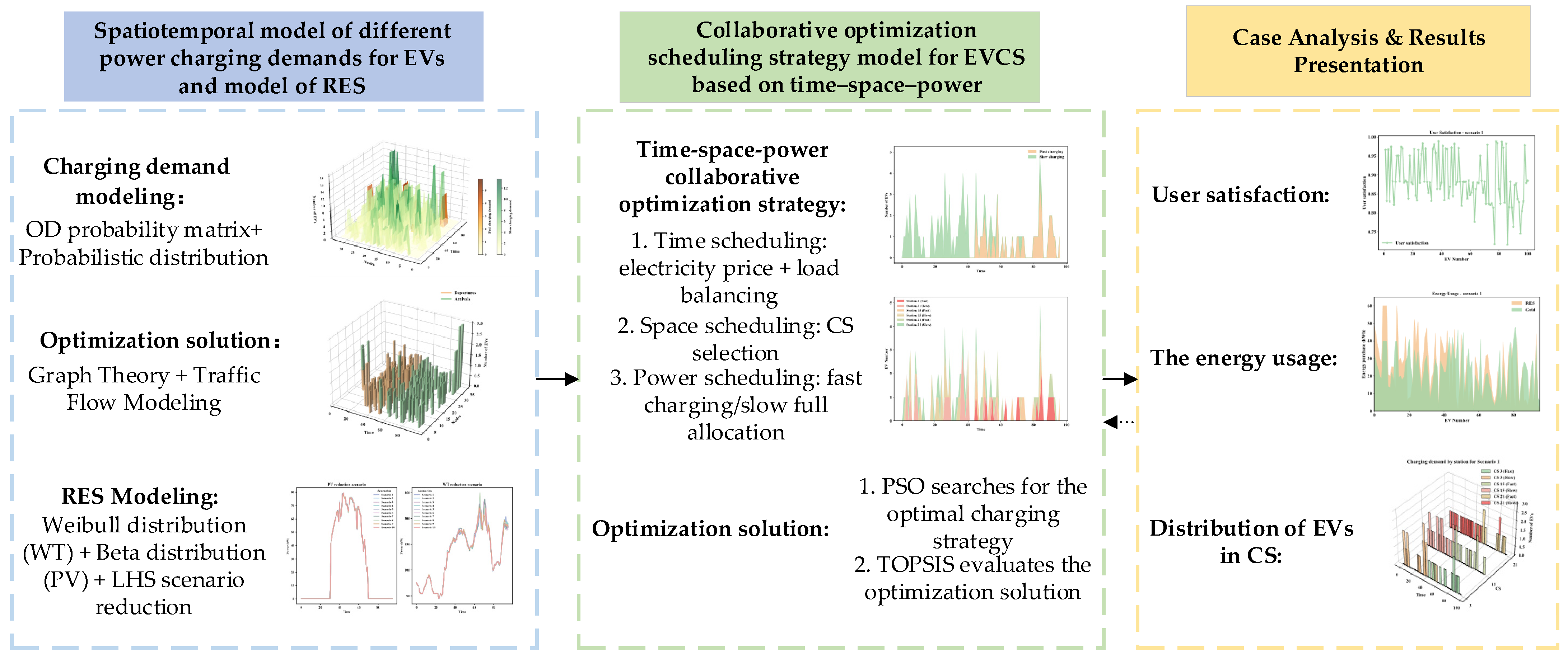
This study proposes a spatiotemporal-power collaborative optimization scheduling framework for EV charging. The framework establishes a comprehensive model for EV charging demand, incorporating the temporal and spatial variations in both fast and slow charging requirements. It also integrates the uncertainties associated with RES, wherein wind power output is modeled using Weibull distributions and solar power output is modeled using Beta distributions. Additionally, a dynamic traffic network simulation is employed to capture the fluctuations in mobility patterns and provide a realistic representation of EV charging demand.

Based on these models, a collaborative optimization scheduling strategy is developed. This strategy dynamically adjusts key variables, including charging station selection, charging time allocation, and power distribution (fast and slow charging) to optimize the trade-offs between user satisfaction, power purchase costs, and load balancing. The optimization problem is addressed using PSO, with the evaluation of user satisfaction performed through the TOPSIS method. Figure 1 shows the research framework of this paper. The paper is organized as follows:

Section 1 introduces this study’s motivation, highlighting the challenges of EV charging demand, renewable energy integration, and the limitations of current strategies.

Section 2 describes the research methods, including the spatiotemporal model for charging demand, dynamic traffic network, and RES uncertainty modeling.

Section 3 provides the spatiotemporal model for EV charging demand, the dynamic traffic network, and the uncertainty modeling of renewable energy sources.

Section 4 introduces the collaborative optimization scheduling strategy, detailing the objective function, constraints, and solution method.

Section 5 presents the case settings and analysis of optimal scheduling results, discussing the impacts of the proposed approach.

Section 6 summarizes the conclusions, emphasizing the effectiveness of the proposed scheduling strategy in improving user satisfaction, reducing costs, and optimizing load balancing.

3. Spatiotemporal Model of Different Power Charging Demands for EVs and Model of RES

With the increasing adoption of EVs, the spatiotemporal distribution of charging demand poses significant challenges for CS scheduling and grid load management. EV demand fluctuates considerably due to factors such as traffic flow, station locations, and time of day. This study proposes a model that represents the spatiotemporal distribution of charging demand across varying power levels. By integrating a dynamic road network model with an RES uncertainty model, the approach aims to optimize CS scheduling.

3.1. Dynamic Traffic Network Model

To model the spatiotemporal distribution of EV charging demand, this study adopts a graph-theoretic approach to construct a dynamic traffic network model. The model simulates driving behaviors and charging requirements across road segments and time intervals. The transportation network is represented as $G=\left(V,E,K,W,L\right)$,where $V$ is the set of nodes, $E$ is the set of all road segments, $K$ is the set of time periods, $W$ is the set of road segment weights, and $L$ is the set of time period weights. Road segment weights are influenced by factors like capacity, traffic flow, speed limits, road length, and saturation levels [27]. For simplicity, these weights are categorized into intervals to reflect different traffic states. The weight of each road segment $w_{ij}\left(t\right)$ varies by time period $t$ and is adjusted as follows:

$$w_{ij}(t)=w_{ij}(t_0)\cdot j_t$$

(1)

In this model, $w_{ij}(t_0)$ represents the initial road segment weight without the influence of time periods, and $j_t$ is the adjustment factor associated with time period $t$. During peak periods, $j_t$ may be large, while during nighttime periods, it may be small. The weight and capacity of a road segment are influenced by traffic flow, with the saturation level $S_{ij}(t)$ being a key factor for dynamic adjustment. The saturation level of a road segment is the ratio of its capacity to its traffic flow, expressed as follows:

$$S_{ij}(t)={\displaystyle \frac{V_{ij}(t)}{C_{ij}(t)}}$$

(2)

where $C_{ij}(t)$ represents the maximum capacity of a road segment during time period $t$, measured in vehicles per hour $(\mathrm{veh}/\mathrm{h})$. Typically, arterial roads have higher capacity, while feeder roads have lower capacity.$V_{ij}(t)$ represents the traffic flow on a road segment during time period $t$, also measured in vehicles per hour $(\mathrm{veh}/\mathrm{h})$. Higher congestion (i.e., higher $V_{ij}(t)$) leads to larger adjustments in $w_{ij}(t)$. This reflects the impact of congestion on the road segment’s operational capacity, as shown in Equation (2).

The impedance value of a road segment is influenced by factors such as segment length, traffic flow, and saturation level. Assuming the impedance of a road segment is described by the following formula:

$$R_{ij}(t)=t_0\cdot L_{ij}\cdot (1+\alpha \cdot S_{ij}{(t)}^{\beta })$$

(3)

where $t_0$ is the travel time $(\mathrm{s})$, $L_{ij}$ is the length $(\mathrm{km})$ of the road segment from node $v_i$ to node $v_i$, $\alpha$ and $\beta$ are parameters representing the influence of traffic flow on road segment impedance. The impedance value at node $v_i$ is given by the following:

$$Z_i(t)={\displaystyle \sum _{j\in N_i}{w}_{ij}(t)}\cdot R_{ij}(t)$$

(4)

where $N$ is the set of nodes connected to node i.

3.2. Charging Characteristic Simulation

This study models the charging behavior and flow distribution of EVs using the origin–destination (OD) probability matrix, which captures the flow between departure and destination nodes in the network. The initial departure probability for each node is assumed to be uniformly distributed. Let the network have $N$ nodes, and the OD matrix be a $P$ matrix, where $P_{ij}$ represents the departure probability from node $v_i$ to node $v_i$. The sum of each row in the matrix must satisfy the following normalization condition:

$${\displaystyle \sum _{j=1}^N{P}_{ij}}=1, \forall i\in \left\{1,2,\cdots ,N\right\}$$

(5)

In this study, the initial departure probability matrix $P_{ij}$ is assumed to follow a uniform distribution, meaning that the departure probability from each node is equal:

$$P_{ij}={\displaystyle \frac{1}{N}}, \forall i,j\in \left\{1,2,\cdots ,N\right\}$$

(6)

The starting and destination nodes for each EV are assigned based on the OD matrix probability distribution. The process is as follows. For each vehicle $c_k$, a starting node $v_{sta}(k)$ is randomly selected according to the probability distribution $P_{ij}$ from the OD matrix. Then, based on the selected starting node $v_{sta}(k)$, a destination node $v_{sta}(k)$ is randomly chosen according to the corresponding probability. This OD node assignment process can be expressed as follows:

$$v_{sta}(k)\sim P_i, v_{des}(k)\sim P_{ij}$$

(7)

To reflect traffic flow characteristics across different time periods, this study introduces a time-dependent OD probability matrix $P(t)$, which adjusts the flow distribution for each time period $t$ to better align with traffic conditions. Specifically, the time-dependent OD matrix is expressed as follows:

$$P(t)=\left[\begin{array}{cccc}{P}_{11}(t)& P_{12}(t)& \cdots & P_{1N}(t)\\ P_{21}(t)& P_{22}(t)& \cdots & P_{2N}(t)\\ ⋮& ⋮& \ddots & ⋮\\ P_{N1}(t)& P_{N2}(t)& \cdots & P_{NN}(t)\end{array}\right]$$

(8)

The charging behavior of EV owners is highly uncertain, influenced by factors like departure time, return time, and travel speed, leading to random fluctuations in charging demand [28]. To model this uncertainty, this study uses a probabilistic distribution to capture the spatiotemporal variations in charging demand. Specifically, the daily travel speed of an EV is modeled using a normal distribution [29], with a mean driving speed of 40 and a standard deviation of 1, as described below:

$$f\left(v\right)={\displaystyle \frac{1}{\sqrt{2\pi }{\sigma }_v}}\exp \left({\displaystyle \frac{-{\left(v-{\mu }_v\right)}^2}{2{{\sigma }_v}^2}}\right)$$

(9)

where $v$ represents the daily travel speed $(\mathrm{km}/\mathrm{h})$, ${\mu }_v$ is the mean daily driving speed, and ${\sigma }_v$ is the standard deviation of the daily driving speed. The initial state of charge (SOC) of an EV on a daily basis can be represented using a normal distribution [30], with a mean SOC of 0.6 and a standard deviation of 0.1, as shown in the following formula:

$$f\left(s\right)={\displaystyle \frac{1}{\sqrt{2\pi }{\sigma }_s}}\exp \left({\displaystyle \frac{-{\left(s-{\mu }_s\right)}^2}{2{{\sigma }_s}^2}}\right)$$

(10)

where ${\mu }_s$ is the average daily driving speed, and ${\sigma }_s$ is the standard deviation of daily driving speed. The departure and return times of EVs can be modeled using normal distributions [31]. The mean departure time is 6.9 h with a standard deviation of 1.2 h, while the mean return time is 17.5 h with a standard deviation of 1.8 h, as shown in Equations (11) and (12):

$$f\left(t_{sta}\right)=\left\{\begin{array}{ll}{\displaystyle \frac{1}{\sqrt{2\pi }{\sigma }_{sta}}}\exp \left({\displaystyle \frac{-{\left(t_{sta}-{\mu }_{sta}\right)}^2}{2{{\sigma }_{sta}}^2}}\right)\hfill & 0<t_{sta}\le {\mu }_{sta}+12\hfill \\ {\displaystyle \frac{1}{\sqrt{2\pi }{\sigma }_{sta}}}\exp \left({\displaystyle \frac{-{\left(t_{sta}+24-{\mu }_{sta}\right)}^2}{2{{\sigma }_{sta}}^2}}\right)\hfill & {\mu }_{sta}+12<t_{sta}\le 24\hfill \end{array}\right.$$

(11)

$$f\left(t_{end}\right)=\left\{\begin{array}{ll}{\displaystyle \frac{1}{\sqrt{2\pi }{\sigma }_{end}}}\exp \left({\displaystyle \frac{-{\left(t_{end}+24-{\mu }_{end}\right)}^2}{2{{\sigma }_{end}}^2}}\right)\hfill & 0<t_{end}\le {\mu }_{end}-12\hfill \\ {\displaystyle \frac{1}{\sqrt{2\pi }{\sigma }_{end}}}\exp \left({\displaystyle \frac{-{\left(t_{end}-{\mu }_{end}\right)}^2}{2{{\sigma }_{end}}^2}}\right)\hfill & {\mu }_{end}-12<t_{end}\le 24\hfill \end{array}\right.$$

(12)

In Equations (11) and (12), $\left(t_{sta}\right)$ is the daily departure time $(\mathrm{h})$, $t_{end}$ is the daily return time $(\mathrm{h})$, ${\mu }_{sta}$ and ${\mu }_{end}$ are the mean departure and return times, ${\sigma }_{sta}$ and ${\sigma }_{end}$ are the standard deviations of the departure and return times, respectively.

3.3. RES Output Uncertainty Model

RES output, particularly wind and solar power, is highly uncertain due to meteorological factors. Wind speed, a key factor in wind power generation, typically follows a Weibull distribution. Its probability density function (PDF) is expressed as follows [32]:

$$f_w(v)={\displaystyle \frac{k}{c}}{({\displaystyle \frac{v}{c}})}^{k-1}{e}^{-{\left({\displaystyle \frac{v}{c}}\right)}^k}$$

(13)

where k is the shape parameter, v is the wind speed $(\mathrm{m}/\mathrm{s})$, and c is the scale parameter. The output power of the wind turbine (WT) can be expressed as a function of wind speed v as follows [33]:

$$P_{wt}(t)=\left\{\begin{array}{l}0,V_t<V_{in},V_{out}<V_t\hfill \\ P_{w{t}^{*}}(V_t-V_{in})/(V_{w{t}^{*}}-V_{in}),V_{in}\le V_t<V_{w{t}^{*}}\hfill \\ P_{w{t}^{*}},V_{w{t}^{*}}<V_t<V_{out}\hfill \end{array}\right.$$

(14)

where $V_t$ is the wind speed at t, and the cut-in wind speed, cut-out wind speed, and rated wind speed are denoted as $V_{in},V_{out},V_{W{T}^{*}}$ respectively. $P_{w{t}^{*}}$ represents the rated power of the WT. Given the Weibull distribution of wind speed, the PDF of the WT output power can be derived by mapping the wind speed distribution to the corresponding output power, as shown in Equation (15):

$$f(P_{wt}(t))=\left\{\begin{array}{l}0,P_{wt}(t)<0\hfill \\ 1-\exp \left(-{\left(\left(1+k{P}_{wt}(t)/P_{wt,r}\right)\cdot v_{in}/c\right)}^k\right),0\le P_{wt}(t)\le P_{wt,r}\hfill \\ 1,P_{wt}(t)>P_{wt,r}\hfill \end{array}\right.$$

(15)

For PV systems, solar radiation is the primary factor affecting output. Solar irradiance typically follows a Beta distribution, with its PDF expressed as follows [34]:

$$f_b(r)=\left\{\begin{array}{ll}{\displaystyle \frac{\Gamma (\alpha +\beta )}{\Gamma (\alpha )+\Gamma (\beta )}}{r}^{(\alpha -1)}{(1-r)}^{(\beta -1)}& 0\le r\le 1;\hspace{1em}\alpha ,\beta \ge 0\\ 0& \mathrm{otherwise}\end{array}\right.$$

(16)

where $\Gamma (\alpha )\mathrm{and}\Gamma (\beta )$ is the Gamma function, $\alpha$ and $\beta$ are the shape parameters, $r$ is the solar irradiance. The output power of a PV system can be expressed as follows [35]:

$$P_{pv}(t)={\eta }_{pv}{P}_{p{v}^{*}}{I}_d(t)/I_{d,stc}$$

(17)

where ${\eta }_{pv}$ is the conversion efficiency of PV system, $P_{p{v}^{*}}$ is the rated power of the PV system $(\mathrm{kW})$, $I_d(t)$ is the incident solar irradiance at time $t$ $({\mathrm{W}/\mathrm{m}}^2)$, $I_{d,stc}$ is the standard test condition irradiance $({\mathrm{W}/\mathrm{m}}^2)$. Combining the Beta distribution of solar irradiance, the PDF of the PV output power can be expressed as follows:

$$f(P_{pv}(t))={\displaystyle \frac{\Gamma (\alpha )+\Gamma (\beta )}{\Gamma (\alpha )\Gamma (\beta )}}{\left({\displaystyle \frac{P_{pv}(t)}{P_{pv,r}}}\right)}^{\alpha -1}{\left(1-{\displaystyle \frac{P_{pv}(t)}{P_{pv,r}}}\right)}^{\beta -1}$$

(18)

To simulate the output uncertainty of wind and solar power, this study uses the Latin hypercube sampling method to generate multiple output scenarios. First, wind speed is sampled from the Weibull distribution, and solar irradiance is sampled from the Beta distribution. The generated values of solar irradiance are then processed as follows:

$$V_t=F_{\mathrm{Weibull}}^{-1}(U)$$

(19)

$$I_d(t)=F_{\mathrm{Beta}}^{-1}(U)$$

(20)

where $F_{\mathrm{Beta}}^{-1}$ and $F_{\mathrm{Weibull}}^{-1}$ are the inverse CDFs of the Beta and Weibull distributions, respectively, and $U$ is a uniformly distributed random sample. Using this method, multiple scenarios are generated, each with corresponding wind speed and solar irradiance values, from which power outputs are calculated. After generating numerous scenarios, the K-means clustering method reduces the number of scenarios. The cluster centers are initially selected as K scenarios, and the Euclidean distance between each scenario and the cluster centers is calculated as follows:

$$d_{m,n}=\sqrt{{\displaystyle \sum _{t=1}^T{(P_{wt,m}(t)-P_{wt,n}(t))}^2}}$$

(21)

$$d_{m,n}=\sqrt{{\displaystyle \sum _{t=1}^T{(P_{pv,m}(t)-P_{pv,n}(t))}^2}}$$

(22)

Finally, based on the clustering results, the cluster centers are updated to the mean of all PV and WT scenarios in each cluster. The process is repeated until the cluster centers converge and no longer change significantly.

4. Collaborative Optimization Scheduling Strategy Model for EV Charging Stations Based on Time–Space–Power

With the widespread adoption of EVs, the growing demand for charging services has placed significant pressure on the scheduling and resource allocation at CSs. Balancing grid load, efficiently utilizing RES, and addressing the diverse charging needs of users have become critical challenges. This study proposes a three-dimensional collaborative optimization strategy that integrates time, space, and varying charging power demands. The objective is to enhance user satisfaction, optimize CS resource allocation, and reduce overall charging costs through a comprehensive optimization model.

4.1. Scheduling Strategy

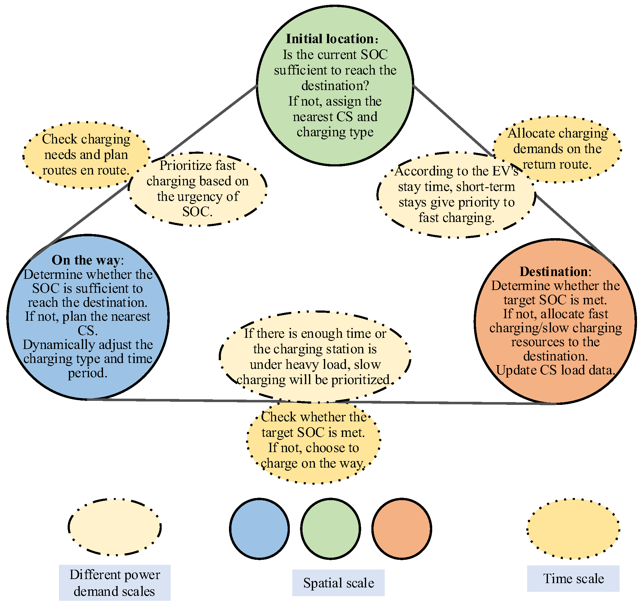
The charging demand of EVs is shaped by the dynamic interplay of time, space, and power dimensions, each critically influencing scheduling decisions. As shown in Figure 2, the time dimension is affected by electricity price fluctuations, peak traffic periods, and CS load, all of which determine the optimal charging timeframe. The spatial dimension is defined by the vehicle’s initial location, travel route, and destination, impacting CS selection. Meanwhile, the power dimension considers battery capacity, charging urgency, and available stopover time, dictating whether fast or slow charging is required. Given these interdependencies, this study proposes a time–space–power collaborative optimization strategy that dynamically adjusts CS selection, charging time, and charging type to maximize user satisfaction while balancing grid load and RES utilization.

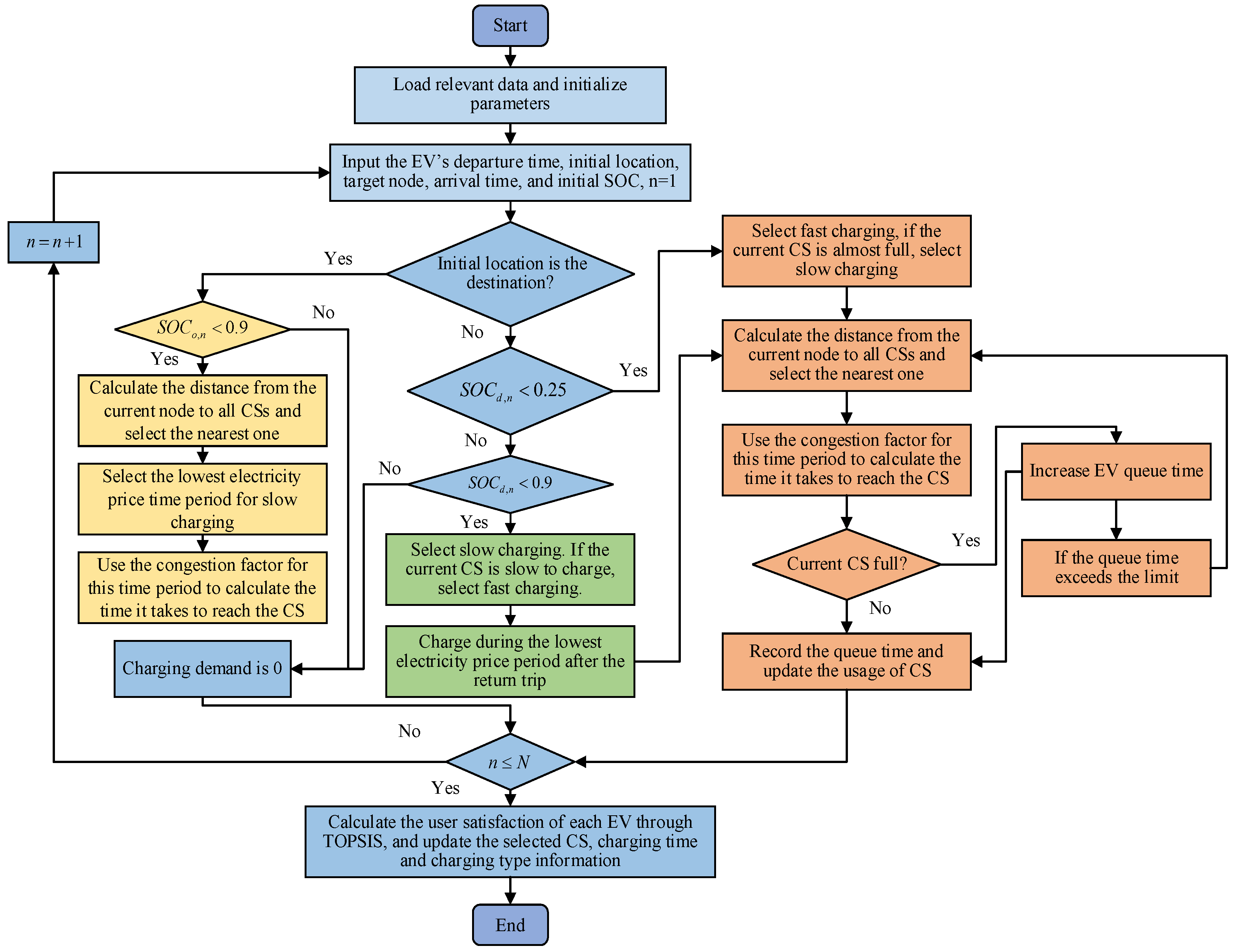
The scheduling process, detailed in Figure 3, follows these steps:

(1).

Input information collection: Gather data on vehicles, CSs, and the power grid.

(2).

Time dimension scheduling: Prioritize low-price periods or fast CSs based on electricity pricing, traffic periods, and charging urgency.

(3).

Spatial dimension scheduling: Based on vehicle location and SOC, select the nearest CS and optimize resource allocation.

(4).

Power demand scheduling: Assign fast or slow CSs based on SOC and urgency, adjusting the proportion of charging types.

(5).

Dynamic resource allocation: Guide EVs to low-load stations or adjust charging time based on station load.

(6).

Execute the scheduling plan: Update SOC, grid energy consumption, charging costs, and user satisfaction.

(7).

Comprehensive optimization: If the objectives are not met, adjust the scheduling strategy until the optimization goals are achieved.

4.2. Objective Function

The objective function in this study integrates three key factors: daily electricity purchase cost, user satisfaction, and CS load balancing, aiming to optimize both charging station operations and economic benefits for EV users.

$$F_{\min }=C_{\mathrm{pow}}+1/S_{\mathrm{sat}}+1/L_{\mathrm{bal}}$$

(23)

where $F_{\min }$ is the target value, $C_{\mathrm{pow}}$ is the electricity purchase cost of the CS $(\mathrm{yuan})$, $S_{\mathrm{sat}}$ is the user satisfaction, $L_{\mathrm{bal}}$ is the load balancing index value. The electricity purchase cost includes the cost of purchasing electricity from the power grid and RES:

$$C_{\mathrm{pow}}={\displaystyle \sum _{t=1}^T(P_{\mathrm{grid},t}\cdot {\lambda }_{\mathrm{grid},t}+P_{\mathrm{res},t}\cdot {\lambda }_{\mathrm{res},t})}$$

(24)

In Equation (24), $P_{\mathrm{grid},t}$ is the grid electricity used in time period $t$ $(\mathrm{kWh})$, $P_{\mathrm{res},t}$ is the RES electricity used in time period $t$ $(\mathrm{kWh})$, ${\lambda }_{\mathrm{grid},t}$ is the grid electricity price in time period $t$ $(\mathrm{yuan}/\mathrm{kWh})$, ${\lambda }_{\mathrm{res},t}$ is the RES electricity price in time period $t$ $(\mathrm{yuan}/\mathrm{kWh})$. For charging station operators, the optimization model minimizes electricity procurement costs by efficiently allocating RES utilization and reducing peak-hour grid dependency. By distributing charging demand more evenly across time and locations, operational costs are lowered while maximizing infrastructure utilization. Furthermore, the model considers user satisfaction by accounting for charging costs, ensuring that optimization also addresses the users’ economic benefits. User satisfaction is determined by queuing time, travel time to the CS, and charging cost, which directly impact the economic benefits for EV users:

(1)

Queuing Time: A penalty term is introduced for longer waiting times, reflecting the user’s negative experience as the wait increases.

(2)

Travel Time: A cost is assigned based on the travel distance to the charging station, with shorter distances yielding higher satisfaction scores.

(3)

Charging Cost: The cost of charging at each station is taken into account, with lower costs corresponding to higher user satisfaction.

The total user satisfaction is calculated as a weighted sum of these factors, with the weight coefficients for queuing time, travel time, and charging cost adjusted according to the time of day. During peak hours (e.g., 07:00–09:00, 17:00–19:00), when traffic congestion and queuing times are higher, more weight is assigned to queuing time and travel time to better reflect their increased impact on the user experience. Conversely, during off-peak hours, when waiting times and travel distances are typically shorter, the weight on charging cost is increased, as users tend to prioritize cost-effectiveness. The satisfaction formula is expressed as follows:

$$S_{\mathrm{sat}}={\displaystyle \sum _{n=1}^{N_{ev}}({\omega }_1\cdot e^{-T_{wait,n}}+{\omega }_2\cdot e^{-T_{tra,n}}+{\omega }_3\cdot e^{C_{pri,n}})}/N_{ev}$$

(25)

In Equation (25), $N_{ev}$ is the total number of EVs, $T_{wait,n}$ is the queuing time of EV n $(\min )$, $T_{tra,n}$ is the time for EV n to go to the CS $(\min )$, $C_{pri,n}$ is the charging cost of EV n $(\mathrm{yuan})$. The time to the CS is calculated by the distance obtained by the shortest path algorithm, the traffic congestion factor, and the EV speed:

$$T_{tra,n}={\displaystyle \sum _{(m,n)\in P_i}{d}_{m,n}\cdot {\kappa }_{m,n,t}/v_{i,\kappa }}$$

(26)

In Equation (26), $P_i$ is the driving path of EV i to the CS, including all connected node pairs $(m,n)$, $d_{m,n}$ is the shortest distance between node m and node n $(\mathrm{km})$, ${\kappa }_{m,n,t}$ is the traffic congestion factor for nodes m and n in time period $t$, $v_{i,\kappa }$ is the speed of EV i under the traffic congestion factor $(\mathrm{km}/\mathrm{h})$. Load balancing is measured by the usage of charging piles in each CS:

$$L_{\mathrm{bal}}=1/N_{cs}\cdot {\displaystyle \sum _{j=1}^{N_{cs}}{\displaystyle \sum _{t=1}^T(U_{j,t}/C_j}}{)}^2$$

(27)

In Equation (27), $N_{cs}$ is the number of CSs, $N_{cs}$ is the actual number of charging piles used at CS j in time period $t$, $C_j$ is the total charging pile capacity of CS j.

4.3. Constraints

The following are the constraints of the charging scheduling model proposed in this paper.

(1)

EV related constraints.

The SOC of the EV must meet the target requirements, and the SOC change is affected by the charging power as follows:

$$SO{C}_{n,T}\ge SO{C}_{tar}, \forall n$$

(28)

$$SO{C}_{n,t+1}=SO{C}_{n,t}+P_{cha,n,t}\cdot \eta /C_{ev}$$

(29)

In the above formulae, $SO{C}_{n,T}$ is the SOC of EV n in the last period, $P_{cha,n,t}$ is the charging power of EV n in time period $t$ $(\mathrm{kW})$, $\eta$ is the charging efficiency, $C_{ev}$ is the battery capacity of the EV $(\mathrm{kWh})$. The charging power of the EV must conform to the type of charging pile currently selected:

$$P_{cha,i,t}\in \left\{P_{fast},P_{slow}\right\}, \forall i, \forall t$$

(30)

In Equation (30), $P_{fast},P_{slow}$ are fast charging power and slow charging power, respectively. The EV must comply with the current path planning when choosing to charge:

$$d_{m,n}\le D_{m,n}, \forall (m,n)\in P_i$$

(31)

In Equation (31), $D_{m,n}$ represents the maximum distance the EV can travel under the current SOC.

(2)

Constraints related to CSs.

Capacity limits for fast charging piles and slow charging piles in CSs:

$${\displaystyle \sum _n{x}_{n,j,t}}\le C_{fast,j}, \forall j, \forall t$$

(32)

$${\displaystyle \sum _n{y}_{n,j,t}}\le C_{slow,j}, \forall j,\forall t$$

(33)

In the above formulae, $x_{n,j,t},y_{n,j,t}$ represent the state variables of the fast charging pile and the slow charging pile, respectively, of the CS j used by EV n in time period $t$, $C_{fast,j}$ and $C_{slow,j}$ represent the total number of fast charging piles and the total number of slow charging piles, respectively, of the CS j. RESs are used first for charging demand, and the rest is provided by the power grid:

$$P_{res,t}+P_{grid,t}\ge P_{total,t}, \forall t$$

(34)

$$P_{res,t}\le P_{res,\max ,t}, \forall t$$

(35)

$$P_{res,t}\ge 0, P_{grid,t}\ge 0$$

(36)

In the above formulae, $P_{total,t}$ is the total charging demand in time period $t$, $P_{res,\max ,t}$ is the maximum RES output available in time period $t$. The charging time period must meet the load conditions of the power grid and the CS:

$${\displaystyle \sum _n{P}_{cha,n,t}}\le P_{\max ,t}, \forall t$$

(37)

where $P_{\max ,t}$ represents the maximum load of the CS in time period $t$. The charging queue time should not exceed a threshold:

$$T_{wait,n}\le T_{wait,\max }, \forall n$$

(38)

where $T_{wait,\max }$ is the maximum allowed waiting time.

(3)

Constraints related to coordinated scheduling of CSs.

In order to achieve efficient coordination among multiple CSs, the following dynamic adjustment constraints are proposed based on the load conditions and fast and slow charging demand distribution of different CSs:

$$C_{fast,j}+C_{slow,j}=C_j, \forall j$$

(39)

$$C_{fast,j}/C_{slow,j}\propto {\displaystyle \sum _n{x}_{i,j,t}}/{\displaystyle \sum _n{y}_{i,j,t}}, \forall j,\forall t$$

(40)

In the above formulae, ${\displaystyle \sum _n{x}_{i,j,t}}$ is the total fast charging demand of CS j in time $t$, ${\displaystyle \sum _n{y}_{i,j,t}}$ is the total slow charging demand of CS j in time $t$. The total load of each CS needs to be dynamically balanced to avoid the overloading of a single CS:

$$P_{total,j,t}/P_{cap,j}\le \delta , \forall j,\forall t$$

(41)

If the load of a CS exceeds the threshold $\delta$, some EVs will be dynamically transferred to other CSs:

$$\mathrm{Re}{\mathrm{direct}}_n\to \arg \underset{j}{\min }\left(P_{total,j,t}/P_{cap,j}\right), \mathrm{if}{P}_{total,k,t}/P_{cap,k}>\delta , \forall k$$

(42)

In the above formula, $P_{cap,j,t}$ is the maximum capacity of CS j, $\delta$ is the load tolerance coefficient of the CS, $\mathrm{Re}{\mathrm{direct}}_n$ indicates that EV n selects a CS with a lower load. Under the premise of meeting the charging needs of EVs, multiple CSs need to coordinate and optimize the use of RES:

$$P_{res,t}+P_{grid,t}\ge P_{demand,j,t}, \forall j,\forall ,t$$

(43)

$${\displaystyle \sum _j{P}_{res,j,t}}\le P_{res,\max ,t}, \forall t$$

(44)

In the above formulae, $\mathrm{Re}{\mathrm{direct}}_n$ represents the total charging demand of CS j at time $t$, $P_{res,j,t}$ represents the amount of RESs used by CS j at time $t$, $P_{grid,t}$ represents the amount of grid power used by CS j at time $t$. If the waiting time at a CS is long, the vehicle is allocated to other CSs through a dynamic usage mechanism:

$$T_{wait,n}={\displaystyle \sum _j{T}_{wait,n,j}}, \forall j$$

(45)

$$\mathrm{Re}{\mathrm{direct}}_n\to \arg \underset{j}{\min }\left(T_{wait,j}\right), \mathrm{if} T_{wait,k}>T_{wait,\max }, \forall k$$

(46)

In the above formulae, $T_{wait,j}$ represents the total queuing time of CS j, and $T_{wait,\max }$ represents the maximum allowed waiting time.

(4)

RES constraints.

$$0\le P_{wt}^t\le P_{w{t}^{*}}$$

(47)

$$0\le P_{pv}^t\le P_{p{v}^{*}}$$

(48)

where, $P_{wt}^t$ and $P_{pv}^t$ represent the output power of the WT and PV at time $t$, and $P_{w{t}^{*}}$ and $P_{p{v}^{*}}$ represent the rated power of the WT and PV.

4.4. Solution Method

To address the EV charging scheduling problem, it is crucial to develop a strategy that effectively balances charging cost, user satisfaction, and load distribution. In this context, a combination of PSO and the TOPSIS method is employed, as illustrated in Figure 4.

PSO is a population-based metaheuristic algorithm that is well-suited for solving high-dimensional nonlinear optimization problems. Its strong global search capability and fast convergence speed make it an effective tool for exploring large solution spaces, which is essential when dealing with dynamic elements, such as traffic conditions, fluctuating energy prices, and distributed charging resources. Given these characteristics, PSO has been widely used in energy management and scheduling problems, demonstrating a balance between computational efficiency and solution quality.

On the other hand, the TOPSIS method is well-suited for decision-making processes involving multiple criteria. In the context of charging scheduling, factors such as waiting time, travel time, and charging price need to be quantified systematically. The TOPSIS method ranks alternatives based on their proximity to the ideal solution, enabling the integration of user preferences into the optimization process.

In light of these considerations, combining PSO and the TOPSIS method allows for an integrated approach that not only optimizes the charging scheduling plan but ensures that user satisfaction is adequately accounted for. This hybrid approach aligns well with the problem at hand and is therefore adopted in this study to achieve a balanced and efficient solution. Furthermore, the proposed approach is designed for large-scale charging networks, which require distributed computing and real-time data integration to effectively manage charging stations and adapt to changing energy demands. The solution process is as follows:

(1).

Data preparation: Load EV operation, CS, road network, RES, and electricity price data.

(2).

PSO initialization: Randomly initialize particle positions and speeds, each representing a scheduling plan. Calculate initial fitness and identify the optimal solution.

(3).

Objective function calculation: Compute charging cost, user satisfaction (via the TOPSIS method for waiting time, driving time, and price), and load balance.

(4).

PSO iteration: Update particle positions and speeds, calculate fitness, and update the individual and global best solutions.

(5).

Convergence check: Terminate when the maximum iterations are reached or the global optimal value stabilizes.

(6).

Output and analysis: Generate the optimal scheduling plan, analyze load distribution, waiting times, and costs, and verify the plan’s effectiveness.

5. Results and Discussion

5.1. Case Setting

In this study, a typical day is selected as the experimental scenario. The simulation is built upon the model formulations detailed in Section 4 (e.g., the objective function in Equation (23) and the constraints in Equations (28)–(48)). The experimental environment is based on a 33-node dynamic road network, with three CSs strategically placed at nodes 3, 15, and 21. Each CS offers both fast charging (30 kW) and slow charging (7 kW) services. Specifically, the number of fast charging piles is set as 1, 2, and 3 for the respective CSs, while the number of slow charging piles is 13, 8, and 15. The simulation considers 100 EVs, each with a battery capacity of 100 kWh, a target SOC of 90%, and a charging efficiency of 90%. All 100 EVs are assumed to participate in the dispatch process. This setup aligns with the energy requirement and charging power constraints specified in Equations (27)–(31). The electricity price is divided into grid and RES electricity prices. The grid electricity price is 0.75 yuan/kWh during the day, 0.33 yuan/kWh at night, and 0.54 yuan/kWh during the standard period, while the RES electricity price is 0.35 yuan/kWh during the day, 0.15 yuan/kWh at night, and 0.24 yuan/kWh during the standard period. These price settings directly influence the cost component of the objective function (Equation (24)). Traffic conditions are modeled by varying congestion coefficients according to time period and road type. During peak hours, the congestion coefficients for main roads and branch roads are 1.3 and 1.2, respectively, and 1.1 and 1.0 during non-peak hours. These coefficients are used to compute travel times (see Equation (26)).

Figure 5 illustrates the topological layout of CSs and the dynamic road network, providing a visual representation of the spatial structure that influences EV charging scheduling. In this topology, the scheduling center coordinates the charging of EVs at three charging stations based on a user satisfaction-oriented collaborative optimization strategy. The charging demand within the stations dynamically responds to real-time changes and prioritizes the use of renewable energy to reduce reliance on the grid. Importantly, the scheduling process is updated every 15 min, allowing the model to capture real-time fluctuations in charging demand and adjust EV allocations accordingly. The overall optimization model is solved using a PSO algorithm combined with the TOPSIS method. The PSO algorithm is configured with 60 particles, 120 iterations, a speed range of [−10, 10], an inertia weight of 0.5, and an acceleration factor of 2. 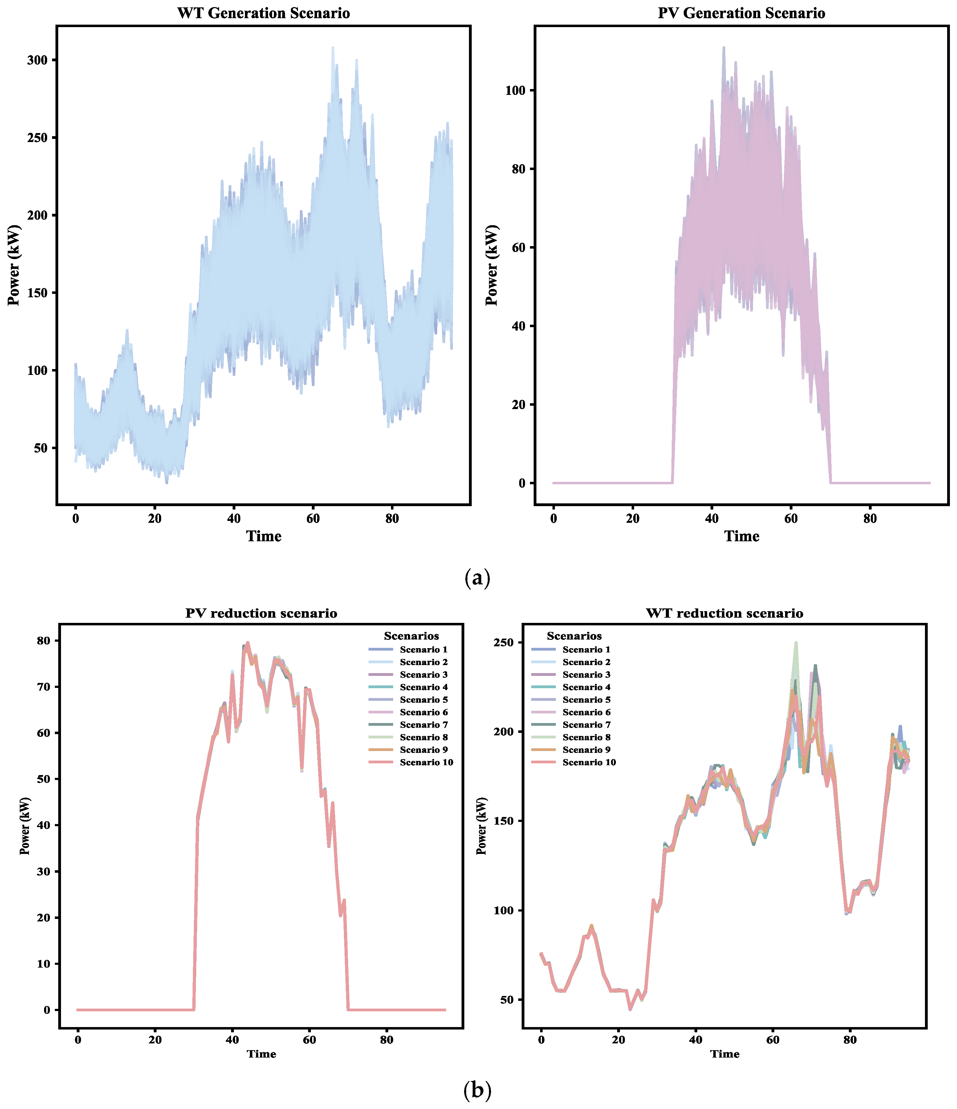Figure 6 depicts the wind and solar output scenarios for typical day, highlighting the fluctuating availability of renewable energy resources. These scenarios are crucial for analyzing the impact of renewable energy integration on the scheduling strategy. To ensure consistency with the constraints and optimization framework, the most likely scenario from the generation and reduction cases is selected for further analysis.

5.2. Spatiotemporal Distribution of Different Power Demand of EVs

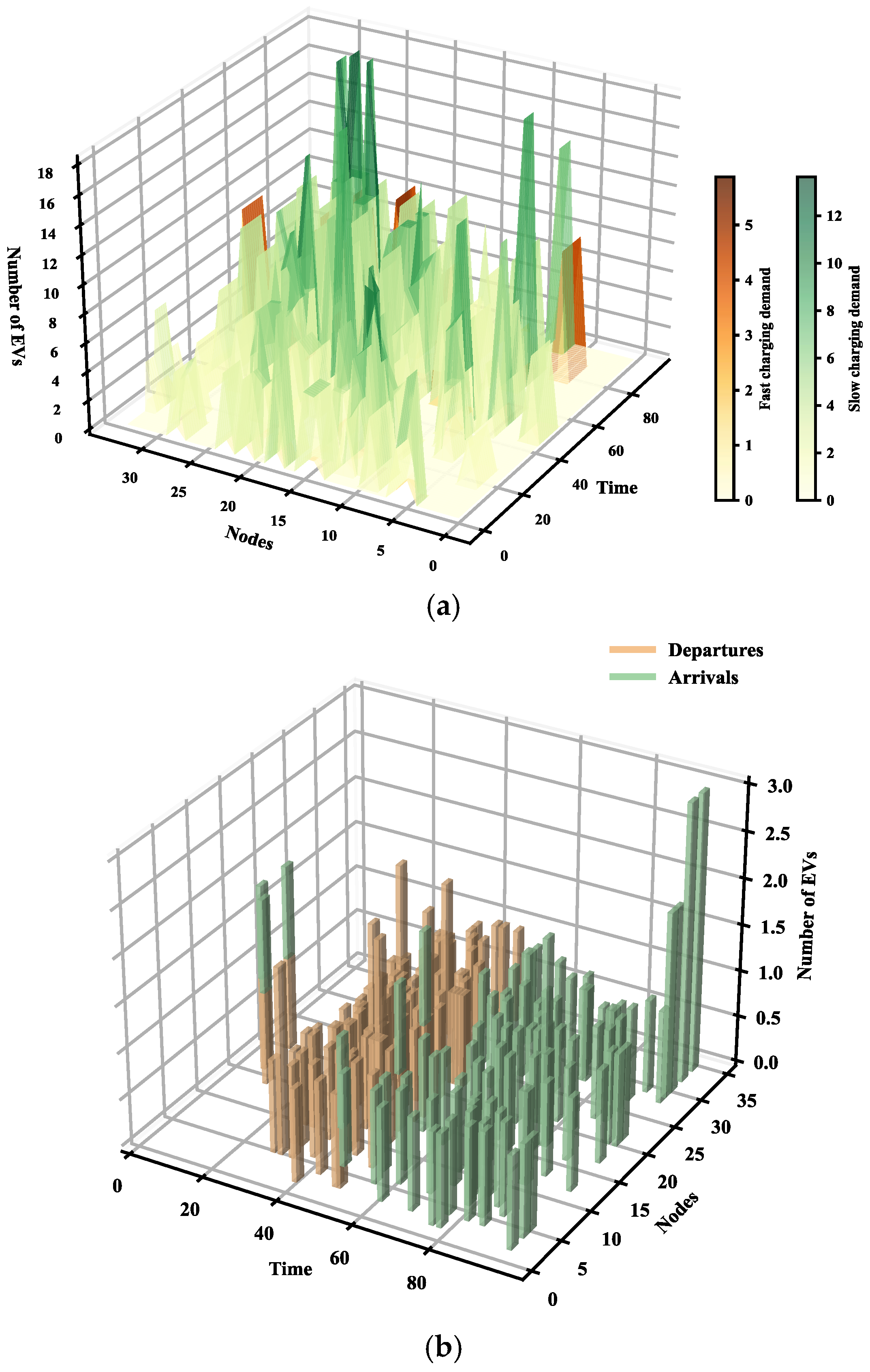
The framework incorporates traffic flow, travel patterns, and charging preferences, allowing the simulation of both fast and slow charging demand across temporal and spatial dimensions. Figure 7a illustrates the spatiotemporal distribution of fast and slow charging demand. Fast charging demand peaks during the morning (07:00–09:00) and evening (15:00–19:00) commuting hours, while slow charging demand is more dispersed and concentrated during off-peak periods. Figure 7b shows the initial locations and destinations of EVs, highlighting the impact of travel behavior on charging demand patterns. 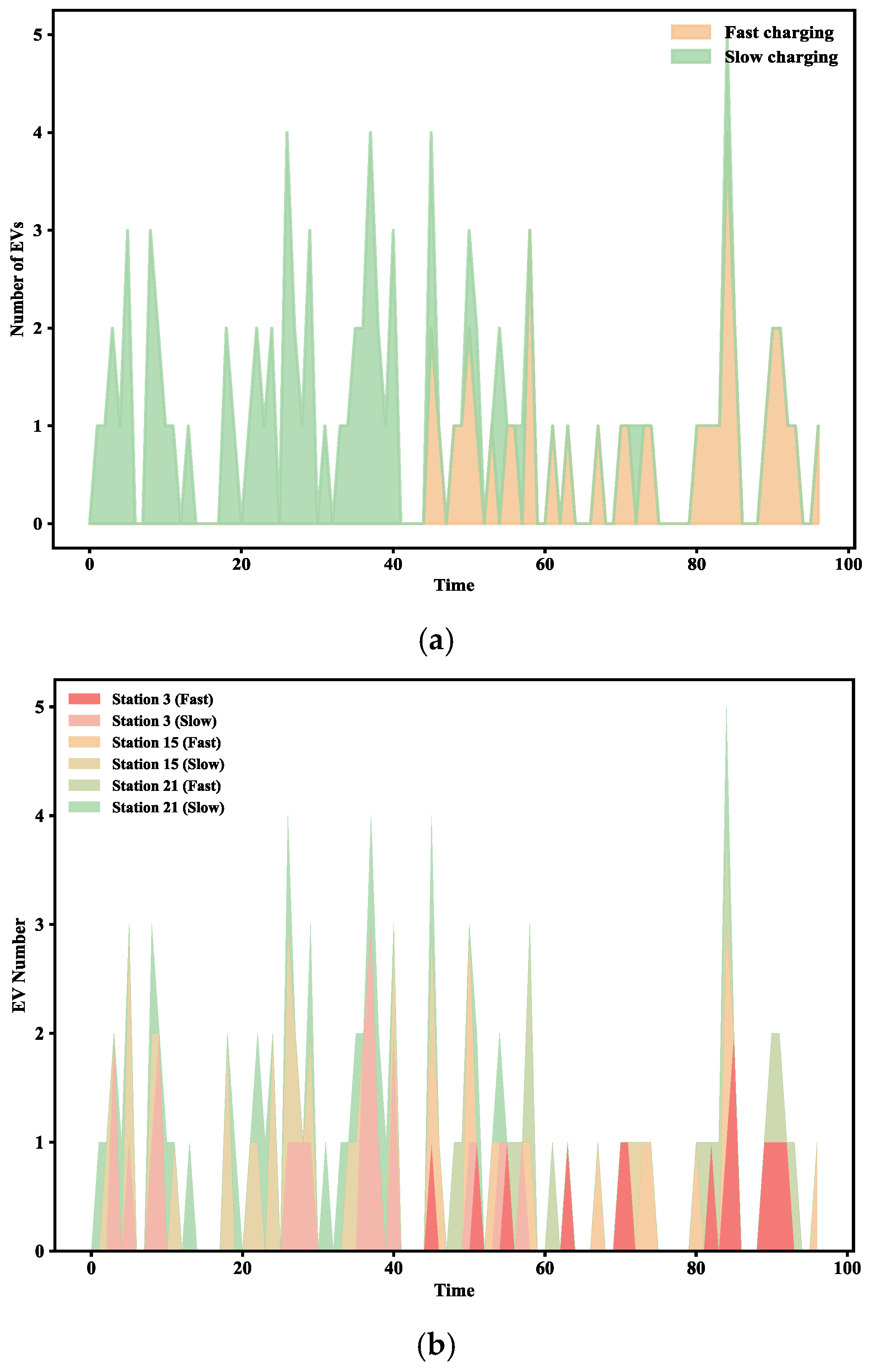Figure 8a further explores the temporal trends in fast and slow charging demand. Fast charging exhibits sharp peaks during high-demand periods, whereas slow charging remains smoother and more evenly distributed. Figure 8b analyzes the distribution of charging demand across stations, revealing that the fast and slow charging demand is relatively balanced among the three stations. The proposed coordinated optimization strategy proves effective in balancing the spatiotemporal distribution of charging demand and managing the scheduling demands for different charging power levels.

5.3. Analysis of Optimal Scheduling Results Based on Time–Space–Power

To validate the effectiveness of the proposed dispatching strategy, we designed a representative day scenario that integrates the dynamics of wind and solar power generation with the spatiotemporal distribution of EV charging demand. Four distinct dispatching scenarios are evaluated to assess the impact of spatial coordination and power flexibility.

Scenario 1 (Time–Space–Multi-Power Coordinated Dispatching): This is the most comprehensive strategy, optimizing charging allocation across temporal, spatial, and power dimensions. Charging stations dynamically coordinate to balance load, cost, and user satisfaction, while leveraging multi-power charging to enhance overall efficiency.

Scenario 2 (Time–Multi-Power Uncoordinated Dispatching): This scenario considers temporal variations and multi-power flexibility but lacks spatial coordination. As a result, each station operates independently, leading to localized congestion and uneven resource utilization.

Scenario 3 (Time–Space–Single-Power Coordinated Dispatching): Here, spatial and temporal coordination are incorporated; however, charging is restricted to a single power level. Although load distribution is improved, the absence of power flexibility limits adaptability and increases waiting times.

Scenario 4 (Time–Single-Power Uncoordinated Dispatching): Representing the least optimized approach, this scenario neither incorporates spatial coordination nor power flexibility. Independent station operation combined with fixed charging power leads to congestion, inefficiencies, and overall suboptimal performance.

Table 1. Optimization results of different scenarios.

Scenario	User Satisfaction	Electricity Purchase Cost (Yuan)	Load Balancing
Scenarios 1	0.935	1693.17	0.784
Scenarios 2	0.864	1805.25	0.658
Scenarios 3	0.912	1753.20	0.753
Scenarios 4	0.850	1856.68	0.643

summarizes the optimization results across these scenarios. Notably, Scenario 1 achieves the highest user satisfaction and the lowest electricity cost, whereas Scenario 4 suffers from significant inefficiencies due to the absence of both coordination and flexibility. Economically, Scenario 1 also reduces charging station operating costs by optimizing load distribution and utilizing renewable energy, leading to lower procurement costs and higher profitability. Users benefit from reduced waiting and charging costs, improving their economic efficiency.

Coordinated dispatching markedly enhances user satisfaction. In Scenario 1, the user satisfaction index reaches 0.935—7.6% higher than that of Scenario 2. It also cuts charging costs by optimizing resource allocation, providing users with greater savings. This finding indicates that coordinated dispatching effectively allocates tasks in response to spatiotemporal variations in charging demand, thereby mitigating resource concentration during peak hours, reducing congestion, and improving the overall user experience. Furthermore, the electricity purchase cost in Scenario 1 is 1693.17 yuan, which is 6.6% lower than the 1805.25 yuan incurred in Scenario 2. By optimizing the distribution of charging loads, collaborative dispatching effectively reduces peak-hour demand and associated procurement costs. Additionally, the load balancing index in Scenario 1 is 0.784—substantially higher than the 0.658 observed in Scenario 2—indicating a 16.1% improvement in achieving an equitable distribution of loads over time and reducing peak load stress.

The advantages of multi-power over single-power dispatching are also evident. Scenario 1 (multi-power dispatching) exhibits a user satisfaction index of 0.935, compared to 0.912 in Scenario 3 (single-power dispatching), a difference of 2.5%. This demonstrates that multi-power dispatching can adaptively adjust power output according to demand, thereby enhancing charging efficiency, reducing wait times, and ultimately improving user satisfaction. In terms of electricity costs, Scenario 3 incurs a cost of 1753.20 yuan—3.5% higher than that of Scenario 1—due to its inability to adjust power output in line with actual demand, leading to higher electricity consumption during certain periods. The load balancing index in Scenario 1 (0.784) also surpasses that of Scenario 3 (0.753) by 4.0%, further confirming that multi-power scheduling contributes to a more balanced load distribution.

By contrast, Scenario 4 performs the worst across all evaluation metrics. The absence of collaborative optimization leads to an uneven distribution of charging tasks, resulting in lower user satisfaction and a diminished load balance index. This also raises operational costs for charging stations, as inefficient resource management increases procurement costs and reduces profitability. This outcome indicates that, without coordinated scheduling, charging stations cannot effectively share resources, which in turn causes excessive load concentration and reduced operational efficiency. 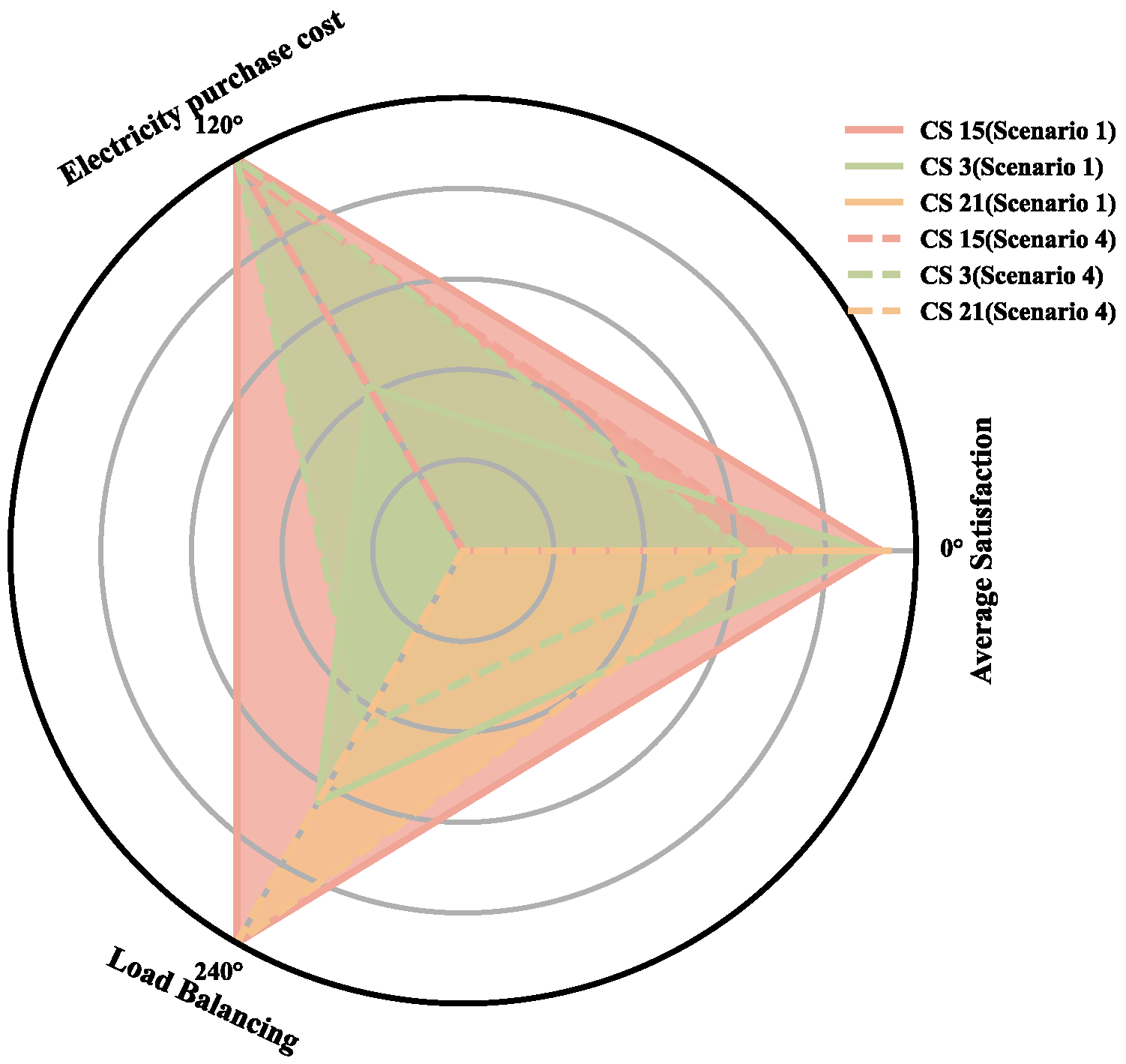Figure 9 illustrates the optimization effects across three CSs under different scheduling scenarios. A radar chart comparison between Scenarios 1 and 4 reveals significant improvements post-implementation: for instance, CS 3 demonstrates marked enhancements in user satisfaction and load balance alongside a substantial reduction in electricity costs; CS 15 experiences an increase in user satisfaction exceeding 30%, a reduction in electricity costs of more than 20%, and an approximate 90% improvement in load balance; similarly, CS 21 shows nearly a 20% increase in user satisfaction, an 18% reduction in electricity costs, and an 85% improvement in load balance.

In summary, the coordinated scheduling strategy based on time–space–power offers significant advantages in improving user satisfaction, reducing electricity purchase costs, and optimizing load balance. The integration of multi-power scheduling with coordinated dispatching enables the system to flexibly respond to spatiotemporal variations in charging demand, thereby enhancing operational efficiency. By contrast, approaches relying solely on single-power or non-coordinated scheduling perform suboptimally, failing to fully leverage charging station resources for effective load management and improved user experience.

5.4. Impact Analysis of Scheduling Strategy Based on Time–Space–Power

To further evaluate the effectiveness of the proposed scheduling strategy, we conducted a comprehensive analysis of the four scheduling scenarios in terms of user satisfaction, energy usage, and charging demand distribution.

Figure 10 shows the distribution of user satisfaction under the four scheduling scenarios, reflecting the impact of different scheduling strategies on user experience. In Scenario 1, user satisfaction is generally high and fluctuates less, maintaining a level above 0.80, indicating that coordinated scheduling can effectively balance the resource allocation between CSs, avoid excessive congestion and uneven resource allocation, and thus maintain high and stable user satisfaction. By contrast, Scenario 2 shows large fluctuations in satisfaction, especially during peak hours, when the satisfaction of some users drops below 0.5. This shows that, in the absence of coordinated scheduling, CSs cannot reasonably coordinate demand, resulting in resource contention and long waiting times, which greatly affects user experience. In Scenario 3, although user satisfaction remains above 0.85 and is relatively stable most of the time, it still decreases compared with Scenario 1. This shows that, although the partial load problem is alleviated through spatial optimization, the flexibility of single-power charging is low and the charging efficiency is not fully improved as with multi-power scheduling. Scenario 4 performs the worst, with generally low user satisfaction and large fluctuations, especially during peak hours, when satisfaction drops below 0.5 for some periods. This result shows that the single-power and uncoordinated scheduling strategy cannot effectively cope with peak demand, resulting in uneven resource allocation, which seriously affects user satisfaction.

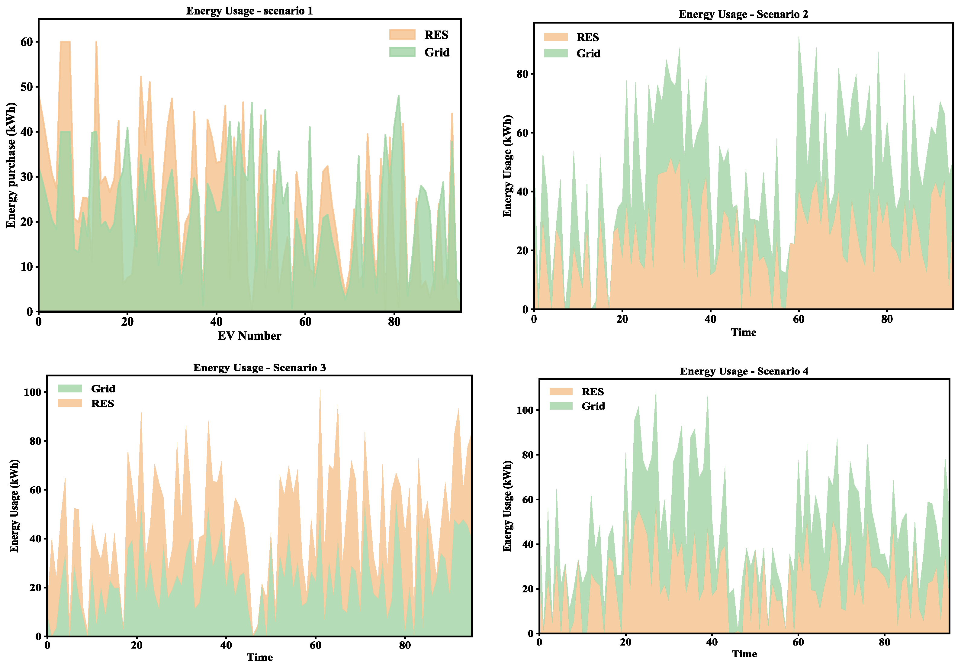
Figure 11 shows the energy usage in four scheduling scenarios, analyzing the distribution of electricity usage from RESs and the power grid. In Scenario 1, the utilization rate of RESs is high and the demand for power purchase from the power grid is relatively low. This shows that coordinated scheduling can effectively match charging demand with the generation of RESs, reduce dependence on the power grid, and thus reduce the cost of power purchase. By contrast, Scenario 2 shows a significant increase in the demand for power purchase from the power grid, especially during peak hours, when the utilization rate of RESs is low in some time periods. The lack of a spatially optimized scheduling strategy makes charging demand concentrated in certain time periods, resulting in insufficient utilization of RESs and increased dependence on the power grid. In Scenario 3, the utilization rate of RESs is still high, but due to the use of single power scheduling, the demand for power purchase from the power grid has increased compared with Scenario 1. The limitation of single power scheduling reduces flexibility, resulting in a higher demand for power purchase from the power grid in certain time periods. Scenario 4 shows the highest demand for power purchase from the power grid and the lowest utilization rate of RESs, especially during peak hours, when the load demand of the power grid increases significantly. This shows that the strategy fails to effectively coordinate charging demand with the supply of RESs, resulting in an increased burden on the power grid and an increase in the cost of power purchase.

Figure 12 displays the number of fast-charging and slow-charging EVs at different charging stations (CS 1, CS 3, CS 15, and CS 21) across various time periods. In Scenario 1, the distribution of charging demand among the CSs is relatively balanced, and the demand for fast charging and slow charging is effectively balanced. Especially during the fast charging period, the demand of CSs 3 and 21 is stable, and the load distribution is relatively uniform, avoiding excessive congestion during peak hours. By contrast, the distribution of charging demand in Scenario 2 is relatively uneven, especially during peak hours, when some CSs have concentrated demand, resulting in congestion. Other CSs have low loads, and the demand of each CS cannot be effectively balanced, resulting in uneven resource utilization. In Scenario 3, there is still a certain imbalance in charging demand, the slow charging demand is especially concentrated in a few CSs (such as CS 3 and CS 15). Although spatial optimization alleviates load concentration, the flexibility of single power scheduling is insufficient, resulting in insufficient resource utilization in some periods. Scenario 4 shows the most serious demand imbalance, especially during peak hours, when some CSs are in excessive demand, while other CSs are not fully utilized, causing excessive congestion and failing to maximize resource utilization efficiency.

6. Conclusions

This paper proposes a time–space–power-based EV charging scheduling strategy, which aims to balance charging demand, improve grid utilization, and enhance user satisfaction. By constructing a 33-node dynamic road network model, simulating the spatiotemporal distribution of charging demand with different power, and comparing and analyzing with the baseline scenario, the effectiveness of the strategy in a typical day scenario is evaluated. The results show that the proposed scheduling strategy shows significant optimization effects on multiple key indicators.

Analysis of the results reveals that Scenario 1—which integrates temporal, spatial, and multi-power coordinated dispatching—achieves the best overall performance. Specifically, Scenario 1 attains a user satisfaction index of 0.935, which is 7.6% higher than that of Scenario 2. The electricity purchase cost in Scenario 1 is 1693.17 yuan, 6.6% lower than the 1805.25 yuan incurred in Scenario 2; while the load balancing index in Scenario 1 is 0.784, marking a 16.1% improvement over Scenario 2’s index of 0.658. This cost reduction benefits both operators, by lowering operational expenses, and users, by reducing charging costs. The advantages of multi-power dispatching are further underscored by the comparison between Scenarios 1 and 3. Although Scenario 3 employs spatial and temporal coordination, its single-power dispatching approach results in a lower user satisfaction index of 0.912 (a 2.5% reduction compared to Scenario 1), an electricity cost of 1753.20 yuan (3.5% higher than Scenario 1), and a load balancing index of 0.753 (4.0% lower than Scenario 1). These figures confirm that multi-power scheduling is essential for adapting to fluctuating charging demands and optimizing overall system performance. By contrast, Scenario 4, which adopts single-power and uncoordinated scheduling, performs the worst across all evaluation metrics. The absence of coordinated optimization in Scenario 4 leads to an uneven distribution of charging tasks, lower user satisfaction, and significant operational inefficiencies. Moreover, Scenario 1 not only optimizes key performance metrics but enhances the utilization of RESs, thereby reducing grid power purchase demand and operating costs, and promoting environmental sustainability. By comparison, the other scenarios exhibit higher dependence on grid power due to less effective mobilization of RESs.

In summary, the proposed scheduling strategy significantly improves user satisfaction, reduces power purchase costs, and optimizes load balancing, offering a solid reference for EV charging scheduling strategies in future smart grids. Future research could explore extending these dynamic models to a larger scale, such as urban or national levels, to better accommodate the growing adoption of EVs and enhance the management of energy transitions. This could involve integrating more complex grid structures, considering varying levels of renewable energy integration, and addressing the impact of long-term trends in EV adoption and energy demand. Additionally, future work could explore the integration of this strategy into current smart grid and IoT-based infrastructures, supporting the sustainable growth of EV networks.