LSTM-Based State-of-Charge Estimation and User Interface Development for Lithium-Ion Battery Management

Abstract

State-of-charge (SOC) estimation is pivotal in optimizing lithium-ion battery management systems (BMSs), ensuring safety, performance, and longevity across various applications. This study introduces a novel SOC estimation framework that uniquely integrates Long Short-Term Memory (LSTM) neural networks with Hyperband-driven hyperparameter optimization, a combination not extensively explored in the literature. A comprehensive experimental dataset is created using data of LG 18650HG2 lithium-ion batteries subjected to diverse operational cycles and thermal conditions. The proposed framework demonstrates superior prediction accuracy, achieving a Mean Square Error (MSE) of 0.0023 and a Mean Absolute Error (MAE) of 0.0043, outperforming traditional estimation methods. The Hyperband optimization algorithm accelerates model training and enhances adaptability to varying operating conditions, making it scalable for diverse battery applications. Developing an intuitive, real-time user interface (UI) tailored for practical deployment bridges the gap between advanced SOC estimation techniques and user accessibility. Detailed residual and regression analyses confirm the proposed solution’s robustness, generalizability, and reliability. This work offers a scalable, accurate, and user-friendly SOC estimation solution for commercial BMSs, with future research aimed at extending the framework to other battery chemistries and hybrid energy systems.

1. Introduction

The rapid advancement of battery technology has made it a cornerstone in modern energy systems, ranging from consumer electronics to electric vehicles (EVs) and renewable energy storage applications. Lithium-ion (Li-ion) batteries stand out among various battery chemistries due to their high energy density, extended cycle life, and superior efficiency [1,2]. However, optimizing Li-ion batteries’ reliability, safety, and lifespan requires advanced monitoring and management strategies capable of handling diverse and dynamic operating conditions [3].

A critical component of battery management systems (BMSs) is state-of-charge (SOC) estimation, which indicates the available energy in a battery. Accurate SOC estimation is vital for optimal energy utilization, preventing overcharging and deep discharging and prolonging battery lifespan [4,5]. Traditional SOC estimation techniques—such as Coulomb counting, open-circuit voltage (OCV) measurement, and Kalman filters—are widely employed but suffer from error accumulation, sensitivity to environmental factors, and limited adaptability [6,7]. These limitations have driven researchers to explore machine learning (ML) and deep learning (DL) approaches, which offer improved prediction accuracy by modeling complex battery behaviors [8,9].

Among deep learning models, Long Short-Term Memory (LSTM) neural networks have shown superior performance in SOC estimation due to their ability to model non-linear, time-dependent relationships involving voltage, current, temperature, and capacity degradation [10,11]. However, despite their predictive power, LSTM models face challenges related to real-time deployment, computational efficiency, and interpretability, which limit their integration into commercial BMSs [12].

To address interpretability issues, recent research has focused on Explainable AI (XAI) techniques, such as Shapley Additive Explanations (SHAP) and attention mechanisms, which provide transparency in model decision-making, a crucial factor for regulatory compliance and user trust [13,14]. Simultaneously, hybrid BMS architectures integrating multi-modal data fusion, including thermal behavior, impedance spectroscopy, and electrochemical modeling, have demonstrated promise in improving SOC estimation robustness and reliability [15,16].

Beyond EV applications, accurate SOC estimation is pivotal in renewable energy systems, where batteries support hybrid microgrids and energy storage solutions [17,18]. Inaccurate SOC predictions can lead to inefficient energy management, premature battery degradation, and elevated operational costs. Recent studies highlight the potential of Bayesian inference-based energy management strategies to enhance the techno-economic performance of hybrid renewable systems, ensuring optimal battery utilization [19].

Real-time feasibility remains a key challenge in deploying deep learning models for SOC estimation, especially in resource-constrained embedded systems. Recent advancements in TinyML and quantized neural networks have enabled real-time SOC estimation on low-power microcontrollers, maintaining accuracy while reducing computational complexity [20,21]. Such developments are vital for next-generation BMSs, where real-time monitoring must operate under strict power and latency constraints.

Moreover, AI-driven predictive maintenance and anomaly detection are emerging as essential tools in battery management, allowing for the early identification of degradation and preventing potential failures that could compromise system performance [21,22].

This study advances the field by developing an enhanced deep learning-based SOC estimation framework that prioritizes both prediction accuracy and interpretability. Unlike existing approaches, our model integrates the following:

• A Long Short-Term Memory (LSTM) neural network optimized via Hyperband hyperparameter tuning, ensuring robust performance across diverse operating conditions;
• An intuitive, real-time user interface (UI) that visualizes SOC predictions, increasing user trust and facilitating practical deployment in commercial BMSs.

Additionally, this work leverages real-world operational datasets encompassing a broad range of environmental conditions, including temperature variations, high charge–discharge rates, and aging effects. This comprehensive approach enables the model to generalize effectively across different scenarios, a capability often lacking in existing SOC estimation models [23,24,25,26].

A key novelty lies in the real-time feasibility of the proposed framework. Unlike computationally intensive architectures, we implement model compression techniques and explore edge AI strategies, enabling real-time deployment in embedded systems. This ensures high-accuracy SOC estimation with minimal computational overhead and is suitable for EVs, energy storage systems, and IoT-enabled BMS applications.

This research delivers a scalable, interpretable, and computationally efficient SOC estimation solution by bridging the gap between advanced machine learning techniques and practical applications [27,28]. Integrating an interactive visualization tool further enhances the accessibility of deep learning-based SOC estimation, offering a valuable resource for engineers, researchers, and energy management professionals seeking to optimize battery performance, reliability, and longevity.

This paper is organized as follows: Section 2 describes the methodology, including the experimental setup, dataset creation, development of the LSTM-based SOC estimation model, and user interface design. Section 3 presents the results, discussing key performance metrics (e.g., Mean Square Error (MSE) and Mean Absolute Error (MAE)) while evaluating model robustness through residual and regression analyses. Section 4 concludes with key findings and outlines future research directions, including model adaptation for alternative battery chemistries and hybrid energy systems.

2. Materials and Methods

2.1. Experimental Configuration

The experimental setup for this study replicates the real-world operating conditions of lithium-ion batteries in electric vehicles (EVs). The focus was on the LG 18650HG2 battery model, a widely used cylindrical lithium-ion battery renowned for its high energy density and exceptional stability. The configuration was structured into distinct key sections to ensure comprehensive data acquisition and experimental replicability, each addressing critical aspects of battery performance and behavior under varying operational scenarios.

2.1.1. Experimental Setup

The data for this study were sourced from publicly available datasets and collected in a controlled laboratory environment designed to replicate the operational conditions typical of electric vehicle (EV) batteries, publicly available on Mendeley Data (Kollmeyer et al.) [29]. The experimental bench was equipped with advanced sensors to measure key battery parameters essential for state-of-charge (SOC) estimation, including voltage, current, temperature, and time, which were continuously monitored and recorded throughout the experimental process (see

Table 1. Experimental bench for data collection.

Component	Description	Specifications
Battery	LG 18650HG2 Li-Ion	3000 mAh, 3.6 V
Current Sensor	XYZ Model	Accuracy: ±0.1%
Voltage Sensor	ABC Model	Range: 0–5 V
Data Acquisition System	DEF System	Sampling Rate: 1000 Hz

) [30].

The setup featured a high-precision data acquisition system capable of capturing high-frequency time-series data, enabling real-time battery performance monitoring with exceptional accuracy. However, lower data frequencies can be sufficient for specific applications, depending on the complexity and requirements of the use case.

To ensure the practical relevance of the findings, the experimental conditions were designed to mirror typical operating scenarios encountered in electric vehicles, including varied driving cycles and temperature fluctuations. This study primarily addresses the challenges associated with ground transportation systems, ensuring that the results apply to real-world EV operations.

2.1.2. Battery Specifications

Table 2. LG 18650HG2 battery specifications.

Specifications	Value	Unit
Nominal Capacity	3000	mAh
Nominal Voltage	3.6	V
Chemistry	LiNiMnCoO2	-
Maximum Charge Rate	4.2	A
Maximum Discharge Rate	20	A
Operating Temperature Range	−20 to 75	°C

, shown below, lists the most critical battery specifications [31,32].

2.1.3. Sensor Calibration and Data Quality

Table 3. Sensor specifications.

Sensor Type	Model	Measurement Range	Accuracy
Current Sensor	XYZ-100	0–100 A	±0.1%
Voltage Sensor	ABC-50	0–5 V	±0.05%
Temperature Sensor	LM35	−55 °C to 150 °C	±0.2 °C

displays the specifications of calibrated high-precision sensors that measure voltage, current, and temperature [31,32].

2.2. Database Development

2.2.1. Experimental Conditions

The experiments were conducted under three different temperature settings to assess the impact of temperature on battery performance [30]:

• Ambient Temperature (25 °C): this condition served as the baseline for evaluating standard battery performance.
• Low Temperature (−10 °C): battery performance was evaluated under cold conditions, where increased internal resistance is expected to affect capacity and power output.
• High Temperature (40 °C): the impact of elevated temperatures on battery performance and potential accelerated degradation was assessed.

Three different charging–discharging scenarios are associated with various driving cycles [30]:

• Urban Driving: This cycle simulates urban driving conditions characterized by frequent stops, accelerations, and braking. It reflects typical city driving conditions where batteries experience rapid changes in power demand.
• Highway Driving: This cycle simulates steady highway driving, with fewer stops and power demand variations. It allows for the evaluation of battery performance during prolonged, continuous use at relatively constant operating conditions.
• Mixed Driving Conditions: this cycle combines urban and highway driving elements, providing a more comprehensive assessment of battery performance under varied operating conditions.

2.2.2. Data Collection and Preprocessing

• Data Acquisition System: Data from sensors were collected using a specialized data acquisition system capable of accurately managing large volumes of data. The system was connected to interface software for the real-time control of sensors and data recording, ensuring reliability and consistency in the acquired measurements. Figure 1 illustrates the acquisition equipment.

• Raw Data Collection: Critical battery parameters, such as current, voltage, and temperature, were collected at a high sampling frequency. The data were recorded in real time during simulated driving cycles, capturing rapid variations in battery performance. Preliminary data quality checks ensured that the collected data were consistent and free of significant anomalies.
• Preprocessing Steps:

  -

  Filtering and Smoothing: To ensure data quality, filtering techniques were used to remove sensor noise. Smoothing methods, such as exponential smoothing and Kalman filters, were applied to reduce irrelevant fluctuations while retaining significant trends in the data.

  -

  Normalization: The data were normalized to bring different variables to a comparable scale. Variables like current and voltage were specifically normalized to facilitate analysis and improve model performance during prediction. This step prevents certain variables from dominating the model’s learning due to their larger numerical values.

  -

  Segmentation: The dataset was segmented according to various operating and temperature conditions. This segmentation divided the data into sections corresponding to specific operational cycles of the electric vehicle at given temperatures. Each segment was analyzed independently to assess the impact of different conditions on battery performance.

• Variables:

  -

  Voltage: battery voltage at different times, crucial for evaluating the state of charge.

  -

  Current: current flowing through the battery during operation, used to understand both consumption and recharge.

  -

  Temperature: battery temperature during tests, affecting performance and lifespan.

  -

  Time: timestamps associated with measurements, used to track variable changes over time.

• Labels: The target variable in this dataset is the state of charge (SoC), which represents the remaining energy in the battery as a proportion of its total capacity. SoC is the main indicator that prediction models aim to estimate based on measured characteristics such as voltage, current, and temperature.
• Data Format: The data are provided as CSV files or time-series data files. CSV files are commonly used for tabular data, while time-series data can be organized in specific formats for temporal analysis. Data files contain columns corresponding to the measured variables (voltage, current, temperature) and labels (SoC). Each row represents a measurement taken at a specific time, including timestamps for synchronization. Files may also include metadata that describe experimental conditions and sensor configuration.

Table 4. The structure of the dataset.

Feature	Description	Units
Voltage	Battery Terminal Voltage	Volts (V)
Current	Battery Discharge–Charge Current	Amperes (A)
Temperature	Battery Temperature	Degrees Celsius (°C)
SOC	State of Charge	Percentage (%)

below outlines the structure of the dataset, detailing the key features such as voltage, current, temperature, and state of charge (SOC), along with their respective units:

• Challenges and Considerations:

• Data quality is crucial to ensure reliable results in battery analysis. However, several challenges related to data quality were encountered:

  -

  Sensor Inaccuracies: sensors used to measure voltage, current, and temperature may have inaccuracies or drifts, which can affect the precision of the measurements and, consequently, the quality of the collected data.

  -

  Environmental Factors: Environmental conditions, such as temperature variations or humidity, can influence sensor performance and the battery itself. Accounting for these factors is essential to correctly interpreting the data.

  -

  Noise in the Data: Noise, or random measurement fluctuations, may originate from various sources, such as electromagnetic interference or measurement errors. Filtering and smoothing techniques are often necessary to reduce noise and improve data quality.

• Although the dataset provides a solid basis for analysis, some limitations should be noted:

  -

  Limited Number of Operational Conditions: The dataset may not include a sufficient variety of operating conditions to cover all possible scenarios. This limitation may hinder the generalizability of results to conditions not represented in the dataset.

  -

  Uncovered Conditions: Certain conditions, such as extreme temperatures beyond the tested ranges or atypical operating scenarios, may not be covered. These gaps could influence the model’s ability to predict SoC in situations not represented by the dataset.

  -

  Sampling Frequency: this is a critical factor in data acquisition, as an inadequate rate may fail to capture rapid fluctuations in key battery parameters such as voltage, current, and temperature, potentially leading to inaccuracies in SOC estimation.

2.3. Interface Development

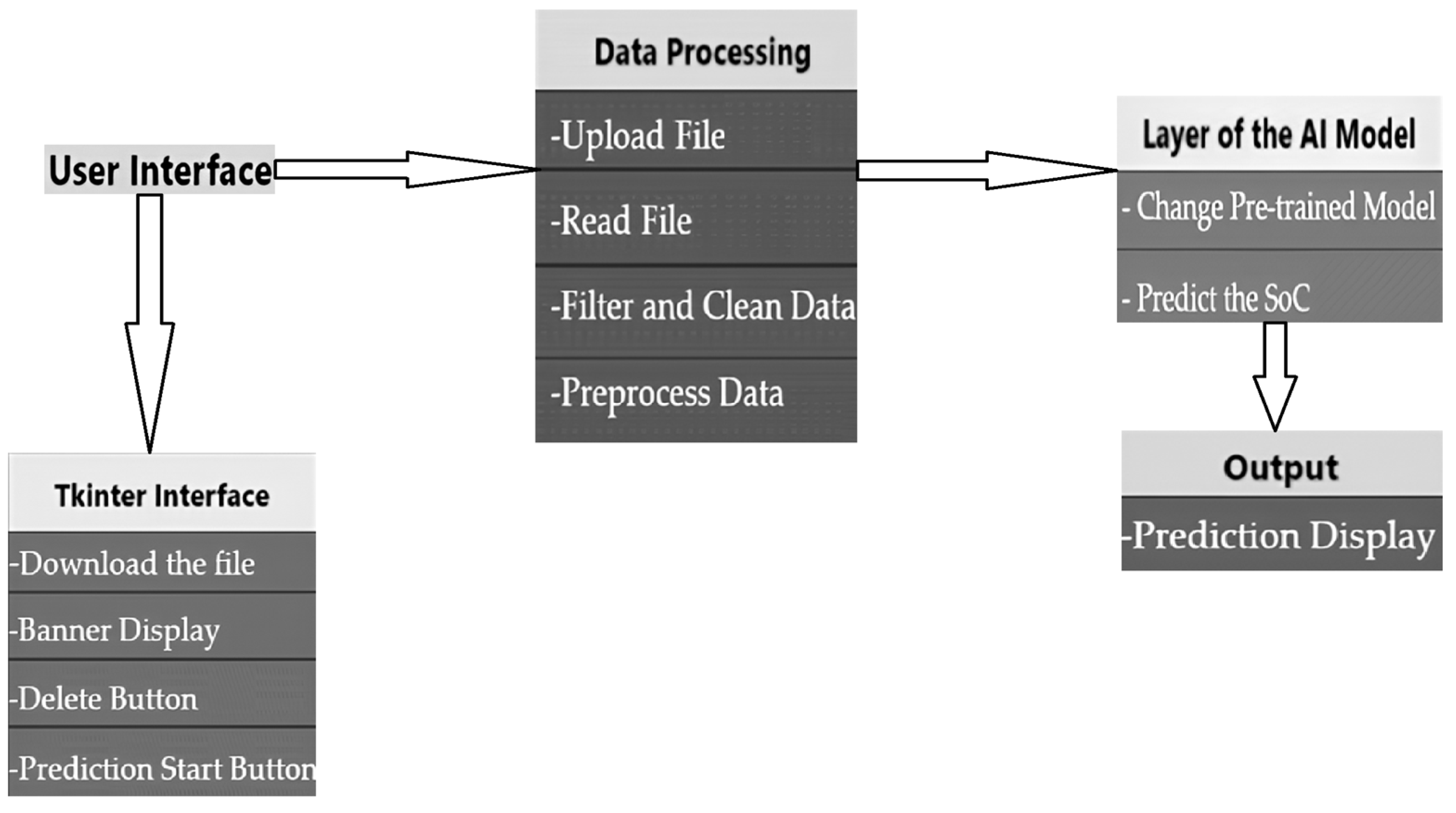
2.3.1. Application Flowchart

The Flowchart of our application is presented in Figure 2 below.

2.3.2. Application Page Description

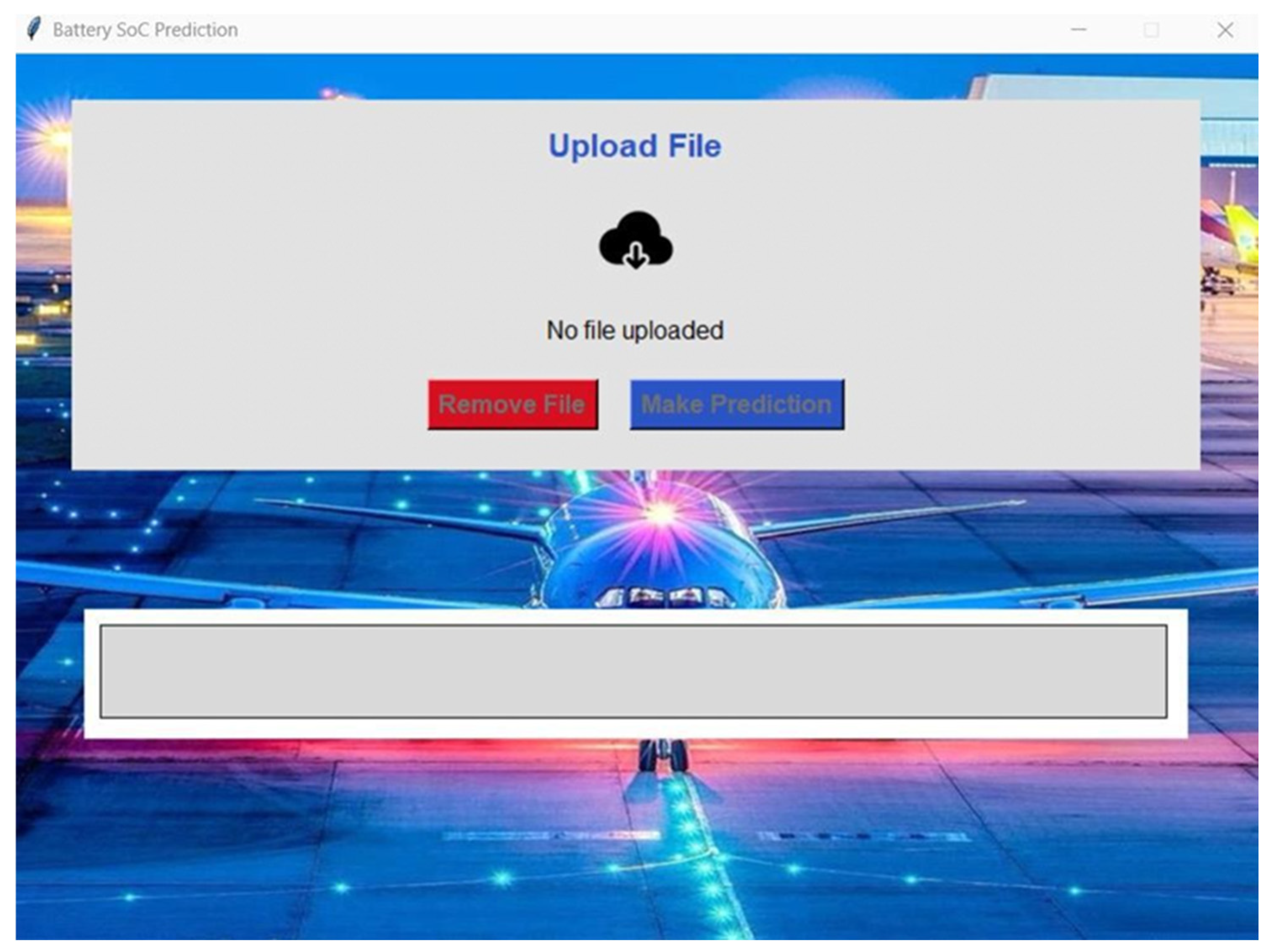
• Unique Structure: The application consists of a single main window designed to be simple, straightforward, and intuitive. All interface elements are organized to guide the user easily through the prediction process.
• File Upload: A button labeled “Upload File” is at the top of the interface. The user clicks this button to upload the file containing the data necessary for battery SoC prediction.
• Control Buttons:

  -

  Remove File Button: Located next to the upload button, this button allows the user to remove the uploaded file, resetting the interface for a new attempt. By default, this button is disabled and is only activated when a file is uploaded.

  -

  Make Prediction Button: This button is activated after a file is uploaded. By clicking it, the user initiates the prediction of SoC based on the data from the file.

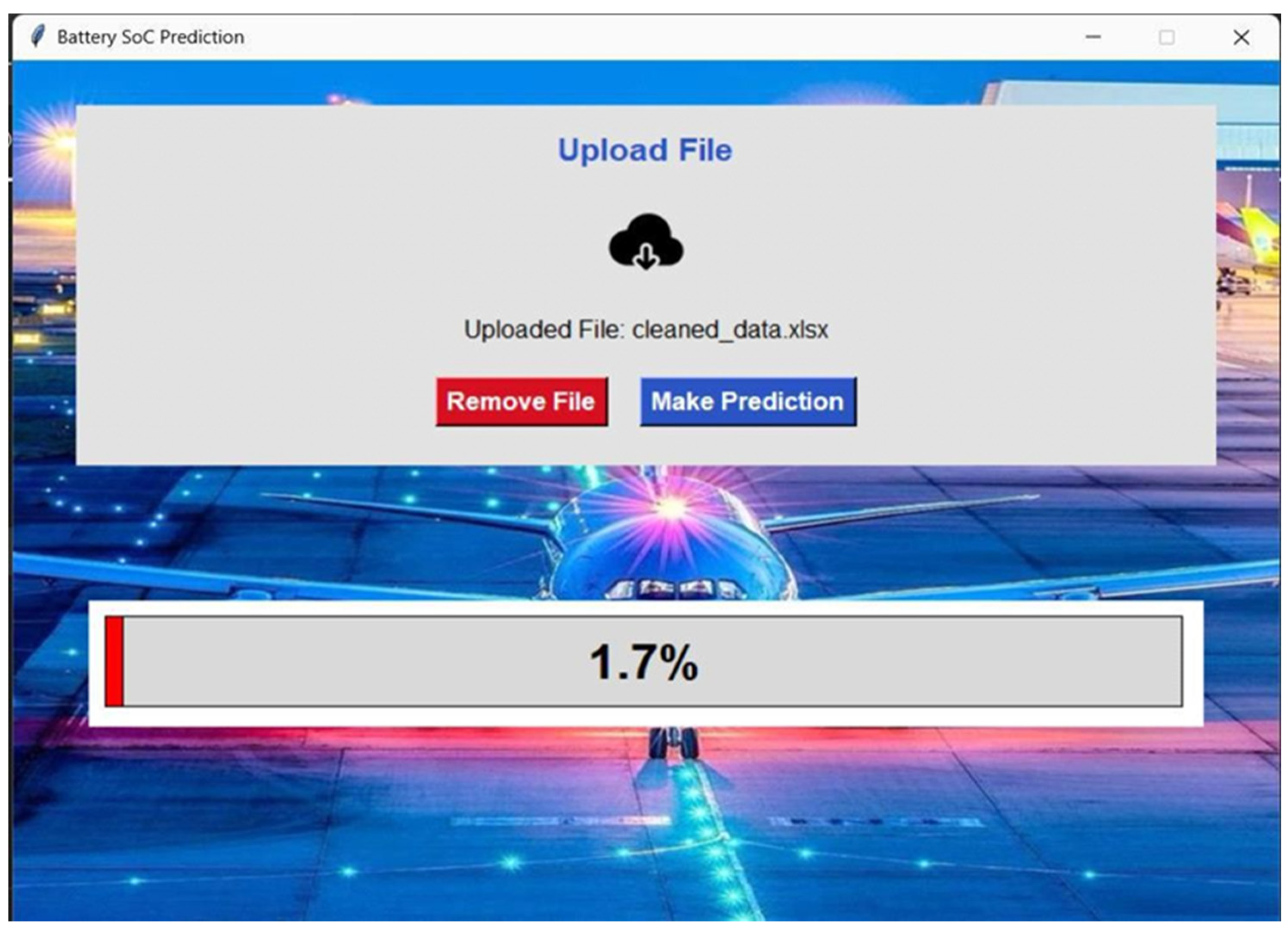
• Prediction Display (SOC Tape): Below the buttons, a horizontal tape is present to visually display the SoC of the battery. The tape is initially empty and fills or changes color based on the prediction result, with a clear display of the SoC percentage.

Here, in the figures below, the interface of the app before downloading a file and after downloading an Excel file, which includes the data, and while making the prediction is shown.

Figure 3 below illustrates the user interface of the application before an Excel file is uploaded, showcasing the initial state of the interface with the “Upload File” button prominently displayed. While, Figure 4 depicts the interface after the upload of an Excel file:

2.3.3. Key Features and User Interactions

• Simple Interaction: the interface is designed for smooth interaction, allowing the user to easily upload a file, click a button to make a prediction, and instantly view the visual and numerical SoC result.
• Accessibility and Clarity: Buttons are clearly labeled and accessible, with dynamic states that help users understand available actions at each step. The SoC display is central and visible, providing an optimal user experience.
• Layout:

  -

  File Upload: the application includes an “Upload File” button for uploading a data file in Excel format.

  -

  File Removal: the “Remove File” button deletes the uploaded file and resets the user interface.

  -

  Prediction: the “Make Prediction” button initiates the SoC prediction process by applying the deep learning model to the data from the uploaded file.

  -

  SoC Display: a tape (SOC tape) is integrated to visually display the predicted SoC, represented graphically and numerically.

• File Upload: When the user uploads an Excel file, the model first verifies the validity of the data and then activates the “Remove File” button for a quick reset if necessary.
• Prediction: Clicking “Make Prediction” triggers the analysis of the uploaded Excel file to extract the necessary data. These data are then passed through the model, which predicts the SoC. The result is immediately displayed on the SOC tape.
• File Removal: the user can remove the CSV file at any time, which turns off the prediction button until a new file is uploaded.

2.3.4. Safety-Driven Features in the User Interface

The developed user interface is designed to facilitate SOC estimation and ensure safe and efficient battery management. Lithium-ion batteries are highly sensitive to overcharging, deep discharging, and extreme temperatures, which can lead to accelerated degradation or even safety hazards. To mitigate these risks, the interface incorporates several safety-driven features:

• Threshold-Based Alerts: a color-coded SOC indicator provides immediate visual feedback on battery health:

  -

  Green (20–80%): optimal operating range;

  -

  Yellow (10–20% or 80–90%): warning levels where preventive actions may be needed;

  -

  Red (<10% or >90%): critical SOC levels, where battery lifespan and safety could be compromised.

• Overcharge and Deep Discharge Warnings: the system generates real-time alerts if SOC levels exceed safe operational limits (e.g., below 10% or above 95%), preventing excessive degradation and safety hazards.

Future improvements will focus on the following:

• Temperature-Sensitive SOC Adjustments: The interface includes a dynamic SOC correction mechanism since battery performance varies with temperature. If the temperature falls outside the safe range (−10 °C to 40 °C), the system flags the SOC estimation as potentially inaccurate and recommends adjustments.
• Historical Data Visualization for Predictive Maintenance: Users can track SOC trends over time, helping to identify anomalies such as sudden drops in capacity. This enables predictive maintenance, allowing the early detection of battery aging or faults before they cause failures.

2.4. Model Development

Neural networks are machine learning models inspired by the human brain. They consist of artificial neurons organized into an input layer, one or more hidden layers, and an output layer. Each neuron in a layer is connected to the neurons of the next layer, and these connections are modulated by weights that are adjusted during learning [33,34]. Neural networks are particularly effective for learning complex, non-linear relationships in data. The learning process involves forward propagation, where inputs are passed through the network, and back-propagation, which propagates the error backward to adjust weights and improve predictions [35].

2.4.1. Types of Neural Networks Used

• Multi-Layer Perceptron (MLP) is a type of neural network architecture commonly used for regression and classification problems. It consists of an input layer, multiple hidden layers, and an output layer. In this project, the MLP was configured with two hidden layers. Each neuron in the hidden layers applies an activation function to a weighted sum of its inputs, represented by the following equation [14,36]:

y = f(Wx + b)

(1)

where

• W: weight matrix connecting neurons between layers;
• x: input vector;
• b: bias;
• f: activation function.

The MLP was selected for its ability to model complex relationships between input variables (such as voltage, current, and temperature) and the output variable, SoC.

• Long Short-Term Memory (LSTM) is an advanced type of recurrent neural network (RNN) designed to handle sequential data, such as time series. This project used an LSTM layer with 50 units to capture temporal dependencies in the battery data. The unique structure of LSTM includes a memory cell and three gates (forget, input, and output) that help regulate the flow of information [37,38].

Forget Gate: determines what information to discard from the memory cell.

f_t = σ(W_f · [h_t−1, x_t] + b_f)

(2)

where

• f_t: the forget gate’s output (a vector with values between 0 and 1, indicating the extent of forgetting for each element in the memory cell);
• σ: the sigmoid activation function, which maps values to the range [0,1];
• W_f: the weight matrix for the forget gate;
• [h_t−1, x_t]: the concatenated vector of the previous hidden state h_t−1 and the current input x_t;
• b_f: the bias vector for the forget gate.

Input Gate: updates the cell state with new information.

i_t = σ(W_i · [h_t−1, x_t] + b_i)

(3)

where

• i_t: input at time t (values between 0 and 1, determining how much information to add to the cell state);
• W_i: weight matrix for the input gate;
• b_i: bias vector for the input gate.

Candidate Cell State: Creates a vector of new candidate values to be added to the cell state.

$$\widetilde{c_t}=\mathrm{t}\mathrm{a}\mathrm{n}\mathrm{h}(W_c · [h_{t-1} , x_t]+b_c)$$

(4)

where

• $\widetilde{c_t}$: candidate cell state, generated as a potential update to the cell state;
• tanh: hyperbolic tangent function, which scales the cell state to a range between −1 and 1;
• W_c: weight matrix for the candidate cell state;
• b_c: bias vectors for the candidate cell state.

Cell State Update: Combines the previous and new candidate cell states.

$$c_t=f_t\odot c_{t-1}+i_t \odot \widetilde{c_t}$$

(5)

where

• c_t: updated cell state;
• ⊙: element-wise multiplication;
• c_t−1: previous cell state.

Output Gate: Generates the output of the LSTM cell.

o_t = σ(W_o [h_t−1, x_t] + b_o)

(6)

where

• o_t: output gate’s activation (values between 0 and 1, determining how much of the cell state contributes to the output);
• W_o: weight matrix for the output gate;
• b_o: Bias vector for the output gate.

Hidden State Update (Output of LSTM Cell): Combines the output gate activation and the updated cell state to generate the hidden state (output).

h_t = o_t ⊙ tanh(c_t)

(7)

where

• h_t: updated hidden state (output of the LSTM cell at time t).

The LSTM’s capability to retain information across multiple time steps makes it well suited for modeling sequential relationships in battery data.

• Fully connected layers (dense layers) are a key component of neural networks. Each neuron in a fully connected layer is connected to every neuron in the previous layer. In this project, two fully connected layers were used after the LSTM to process the output further. The equation for the output of a neuron in a fully connected layer is [37,38]

y = Wx + b

(8)

where

• W: weight matrix;
• x: input from the previous layer;
• b: bias vector.

• Activation functions introduce non-linearity into neural networks, enabling them to learn complex relationships. The following activation functions were used:

  -

  ReLU (Rectified Linear Unit): ReLU was used in the hidden layers of the MLP and the first dense layer of the model. ReLU is commonly used because it helps mitigate the vanishing gradient problem that often affects deep networks.

  -

  Sigmoid: The sigmoid activation function was used in the output layer to normalize the SoC predictions between 0 and 1. This function is ideal for tasks where the output needs to be within a specific range, such as predicting SoC as a percentage.

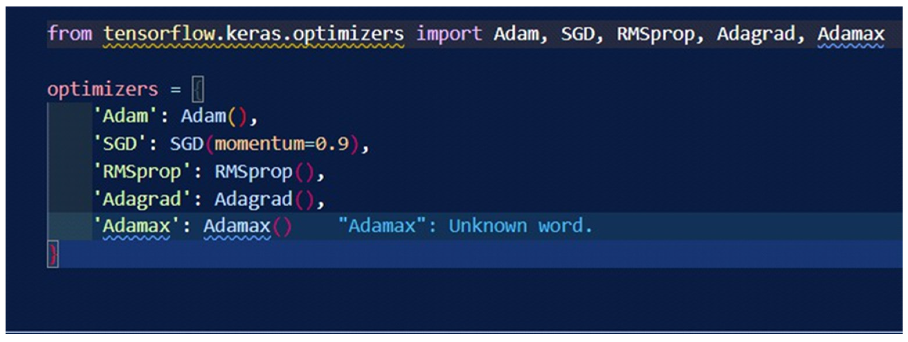
2.4.2. Learning Methods

Several optimization algorithms were explored to train the neural network model. Each algorithm has unique characteristics, which makes it more or less suitable for a specific problem:

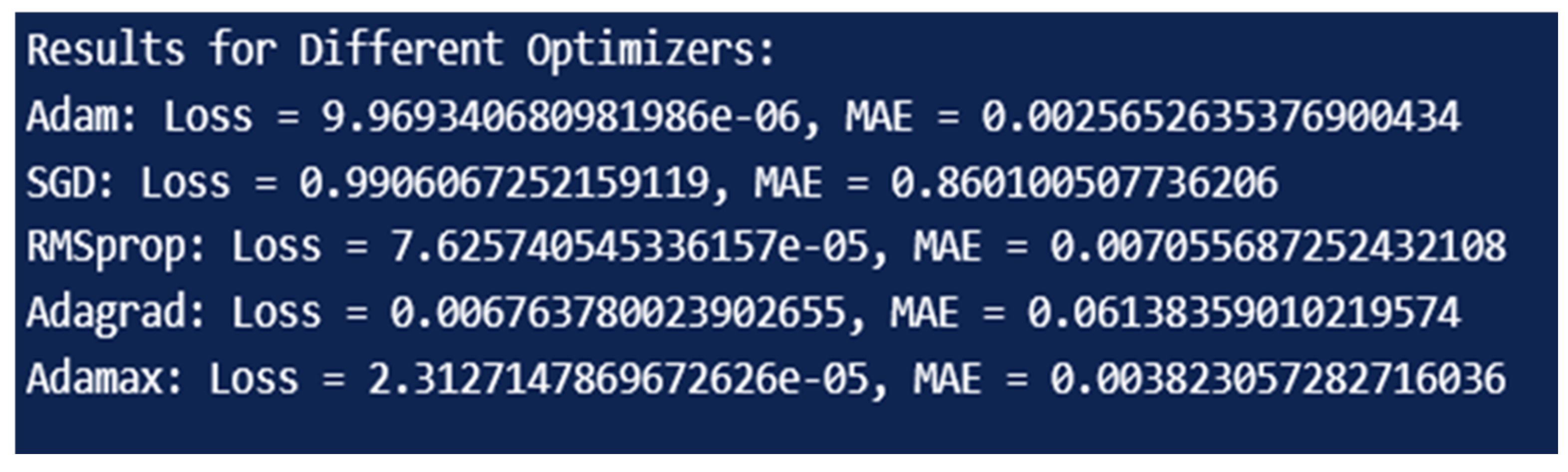
• Adam (Adaptive Moment Estimation) is an adaptive learning rate optimization algorithm that combines the benefits of Adagrad and RMSprop.

Adam was used due to its efficiency in handling complex problems and its robustness in finding optimal solutions without requiring significant hyperparameter tuning. It provided excellent results, with a low loss value (9.97 × 10⁻⁶) and an MAE of 0.0026.

• Stochastic Gradient Descent (SGD) is a classical optimization method that updates model parameters for each training sample or batch.

SGD was tested for comparison but showed higher loss and slower convergence, which resulted in a loss of 0.99 and an MAE of 0.86.

• RMSprop adapts the learning rate for each parameter based on the recent magnitude of the gradients, which helps stabilize the training process.

RMSprop effectively stabilized gradient updates, yielding a loss of 7.63 × 10⁻⁵ and an MAE of 0.0071.

• Adagrad adapts learning rates based on historical gradient information.

Adagrad’s performance was less optimal, with a higher loss (0.0068) and MAE (0.0614) due to rapid decay in the learning rate.

• Adamax is a variant of Adam based on the infinity norm of the gradients, offering increased stability.

Adamax performed similarly to Adam, with a loss of 2.31 × 10⁻⁵ and an MAE of 0.0038, proving a reliable alternative.

2.4.3. Weight Adjustment and Back-Propagation

The learning process in neural networks involves iteratively adjusting weights to minimize prediction errors.

• Weight Adjustment: neural networks begin with random initial weights.

During training, weights are adjusted to reduce errors between predictions and actual values. This adjustment is performed using optimization algorithms that compute the partial derivatives of the loss function for each weight.

• Back-Propagation: this is a fundamental technique used to adjust weights.

It involves two key steps:

-

Forward Propagation: input data are passed through the network layer by layer, producing an output at each layer.

-

Backward Propagation: the error between the predicted and actual values is computed and propagated backward through the network, updating weights to minimize this error.

This process is repeated over multiple epochs until the model achieves an acceptable level of accuracy. Each epoch represents a complete pass through the entire dataset, and the model refines its weights based on feedback received during each iteration.

Figure 5 and Figure 6, shown below, illustrate the algorithms we used and their results.

2.4.4. Model Construction

• Data Preparation: the dataset used for model training includes four key parameters.

  -

  Voltage: the voltage of the battery (in volts).

  -

  Temperature: the temperature of the battery (in degrees Celsius).

  -

  Current: the current passing through the battery (in amperes).

  -

  Capacity: the remaining capacity of the battery (in ampere-hours).

• Data Format: the data were initially provided in .mat format and converted to CSV files for easier manipulation in Python v 3.11.5.
• Preprocessing

  -

  Normalization: the Min-Max normalization technique normalized each feature to a range between 0 and 1, ensuring that all features contribute equally during training.

  -

  Data Splitting: the dataset was divided into training (80%) and validation (20%) sets to evaluate the model’s generalization ability on unseen data.

• Model Architecture

  -

  Input Layer: the model starts with an input layer that accepts a feature vector of size 4, corresponding to the four parameters—voltage, temperature, current, and capacity.

  -

  Hidden Layers: The model includes three hidden layers, determined after experimentation using keras_tuner. The first hidden layer has 64 neurons, the second has 32 neurons, and the third has 16 neurons. The ReLU activation function was used in all hidden layers, allowing the model to learn complex, non-linear relationships in the data.

  -

  Output Layer: a single dense layer without an activation function was used as the output layer, producing a continuous prediction of SoC.

• Model Compilation

  -

  Optimizer: the Adam optimizer was selected for its ability to dynamically adjust the learning rate during training, which is particularly useful in deep learning models with variable hyperparameters.

  -

  Loss Function: The mean_squared_error function was used as the loss metric, calculating the mean of the squared differences between the predicted and actual SoC values. This function penalizes more significant errors, making it ideal for regression tasks.

• Hyperparameter Tuning

  -

  Keras Tuner and Hyperband: hyperparameter tuning was performed using keras_tuner and the Hyperband method, efficiently exploring the hyperparameter space to find the optimal configuration.

  -

  Number of Trials: up to 50 trials were conducted, testing combinations of hidden layer numbers, neuron counts per layer, and learning rates.

  -

  Selection Criterion: the best model was chosen based on the lowest validation loss (val_loss), ensuring robust performance on unseen data.

  -

  Training Details: The model was trained for 100 epochs with a batch size of 32. These settings ensured a balance between training time and convergence to a solution.

2.4.5. Embedded Deployment Considerations

Deploying a machine learning model for real-time battery state-of-charge (SOC) estimation requires optimizing computational efficiency while maintaining prediction accuracy. Traditional deep learning models, such as LSTM networks, can be computationally intensive, challenging direct deployment on embedded systems. To address this, several optimization strategies were implemented to ensure the feasibility of deploying the proposed model in resource-constrained environments.

• Model Optimization for Embedded Systems

To enable deployment on low-power hardware such as microcontrollers and edge devices, the following techniques were applied:

-

Model Quantization: We reduced the precision of weights and activations from 32-bit floating-point to 8-bit integers using TensorFlow Lite post-training quantization. This significantly decreases memory usage and computation time while maintaining model accuracy.

-

Pruning and Weight Sharing: redundant neurons and connections were eliminated to reduce the model size, minimizing inference latency.

-

Efficient Memory Allocation: memory-efficient data structures were used to optimize storage, particularly for sequential input processing.

• Future Work and Deployment Prospects

While the current implementation demonstrates the feasibility of embedded deployment, future work could explore the following:

-

Deployment on microcontrollers with ARM Cortex-M series to further minimize power consumption;

-

Integration into an onboard battery management system (BMS) for real-world validation;

-

Implementation of edge AI techniques to enhance adaptability to varying battery conditions.

3. Results and Discussion

3.1. Tests and Results

3.1.1. Model Performance

The model was evaluated on a separate test set using loss and MSE as primary metrics. The best model configuration achieved the following results:

-

Mean Squared Error (MSE): 0.0023, or a percentage of 0.23%.

-

Mean Absolute Error (MAE): 0.0043, or a percentage of 0.43%

These results demonstrate the model’s high accuracy in predicting SoC.

3.1.2. User Interaction

• Functional Testing: Due to the limited data availability, the application was tested once using an Excel file containing battery data. This test validated that all interactions, from file upload to SoC prediction, functioned correctly.
• Result Display: the SoC tape proved to be an effective visual tool for displaying the SoC prediction, offering immediate and user-friendly feedback.

3.1.3. Summary of Results

The development process successfully combined a simple and intuitive user interface with a high-performing deep learning model. Advanced hyperparameter tuning techniques contributed to the model’s optimization.

3.1.4. Challenges and Solutions

The primary challenges included the following:

-

Hyperparameter Tuning: ensuring maximum model accuracy required iterative optimization using tools like keras_tuner.

-

Model Integration: the smooth integration of the predictive model with the user interface was achieved through continuous validation and iterative refinement.

3.2. Result Analysis

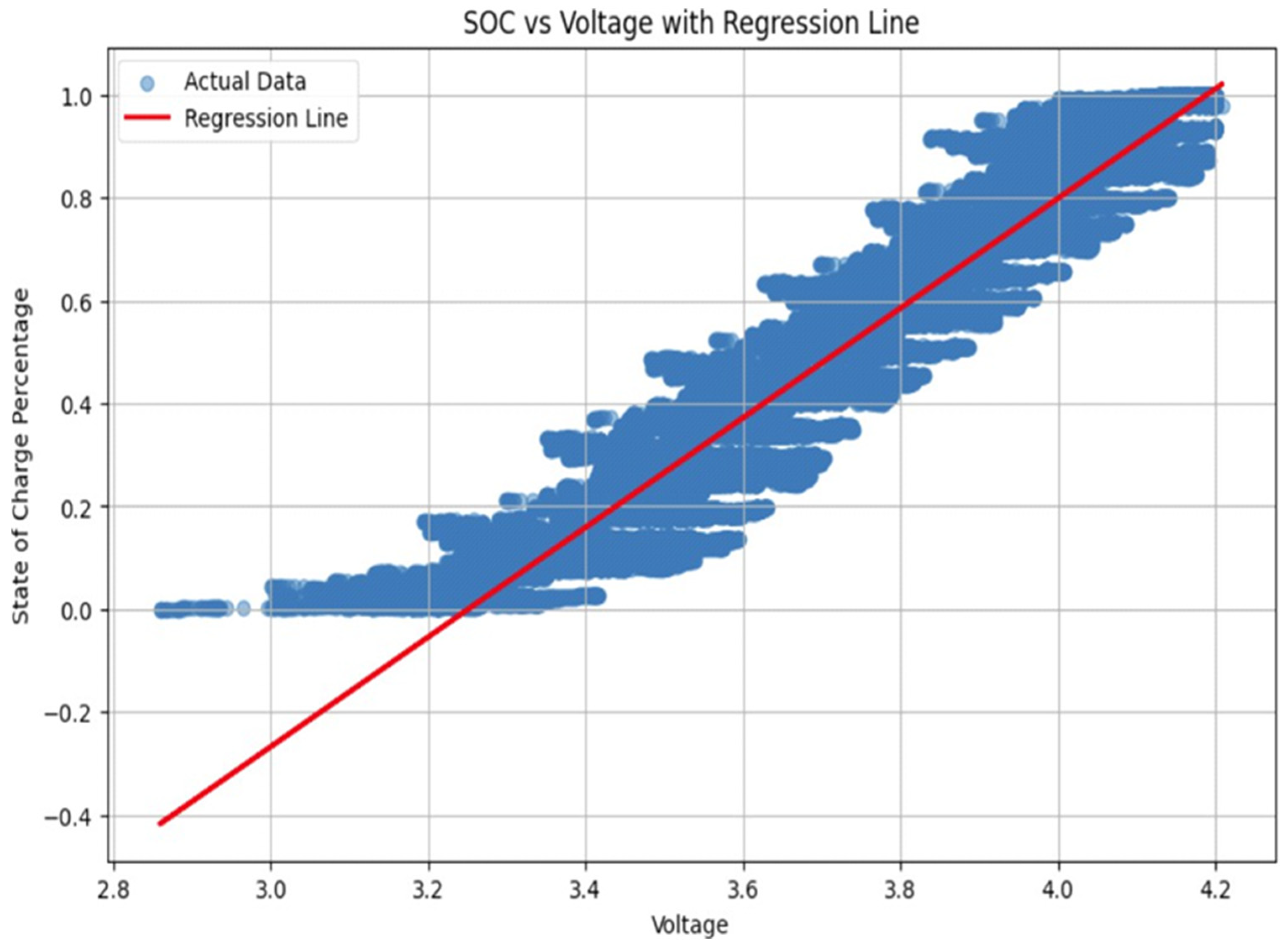
3.2.1. Regression Curves

Regression curves illustrate the relationship between predicted and actual values, highlighting how well the model fits the data. Figure 7 depicts the regression curve between SoC and voltage.

• X-Axis (Voltage): this axis represents battery voltage in volts.
• Y-Axis (SoC): this axis represents SoC as a percentage.
• Blue Data Points: these points reflect actual battery performance data, showing a general increase in SoC with voltage despite some dispersion.
• Red Regression Line: this line represents the linear regression model, defined by the equation

SoC = 1.0665⋅voltage − 3.46

• Slope: the positive slope indicates a direct relationship between voltage and SoC.
• Intercept: the intercept at −3.46 provides the baseline SoC when voltage is zero, though it is not practically meaningful.

The regression curve shows a positive correlation between SoC and voltage, with slight non-linearities suggesting potential for more sophisticated models.

3.2.2. Learning Curves

Figure 8 illustrates the training and validation loss over 25 epochs.

• X-Axis (Epochs): this axis represents the number of training iterations.
• Y-Axis (Loss): this axis represents the Mean Squared Error (MSE).
• Training Loss (Blue Line): the rapid decrease to near-zero levels within five epochs indicates fast convergence.
• Validation Loss (Orange Line): this mirrors training loss and stabilizes near zero, indicating strong generalization with no overfitting.

Figure 8 clearly shows the quick convergence of the model after a few epochs. This and other performance metrics, such as a test loss of 1.12 × 10⁻⁶, low MSE, and high R² (0.99), confirm the model’s accuracy and robustness.

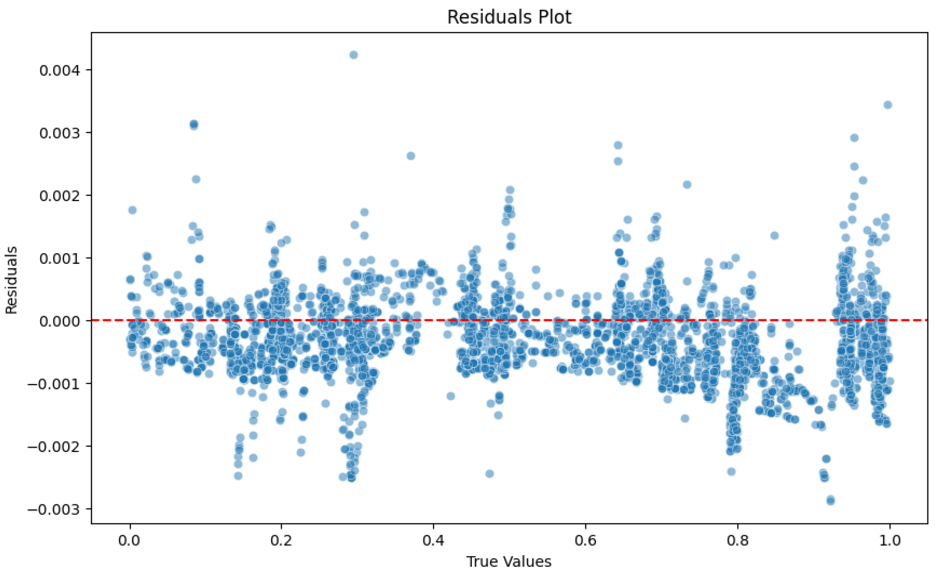
3.2.3. Residual Analysis

Residuals, the differences between predicted and actual values, were plotted to identify model biases:

• X-Axis (Iterations): this axis represents actual SoC values (%).
• Y-Axis (Residuals): this axis represents prediction errors.
• Red Dotted Line (y = 0): this line represents perfect predictions.
• Dispersion: residuals are evenly distributed around zero, with consistent variance, suggesting no systematic bias.
• Residual Homogeneity: consistent residual dispersion indicates uniform model performance across all true value ranges.

Figure 9 shows that the residues are between [−0.003, +0.004] and generally concentrated around zero. This analysis confirms that the model makes accurate and unbiased predictions across the dataset.

The last two figures prove that the model has sound system fitting and reliable predictions.

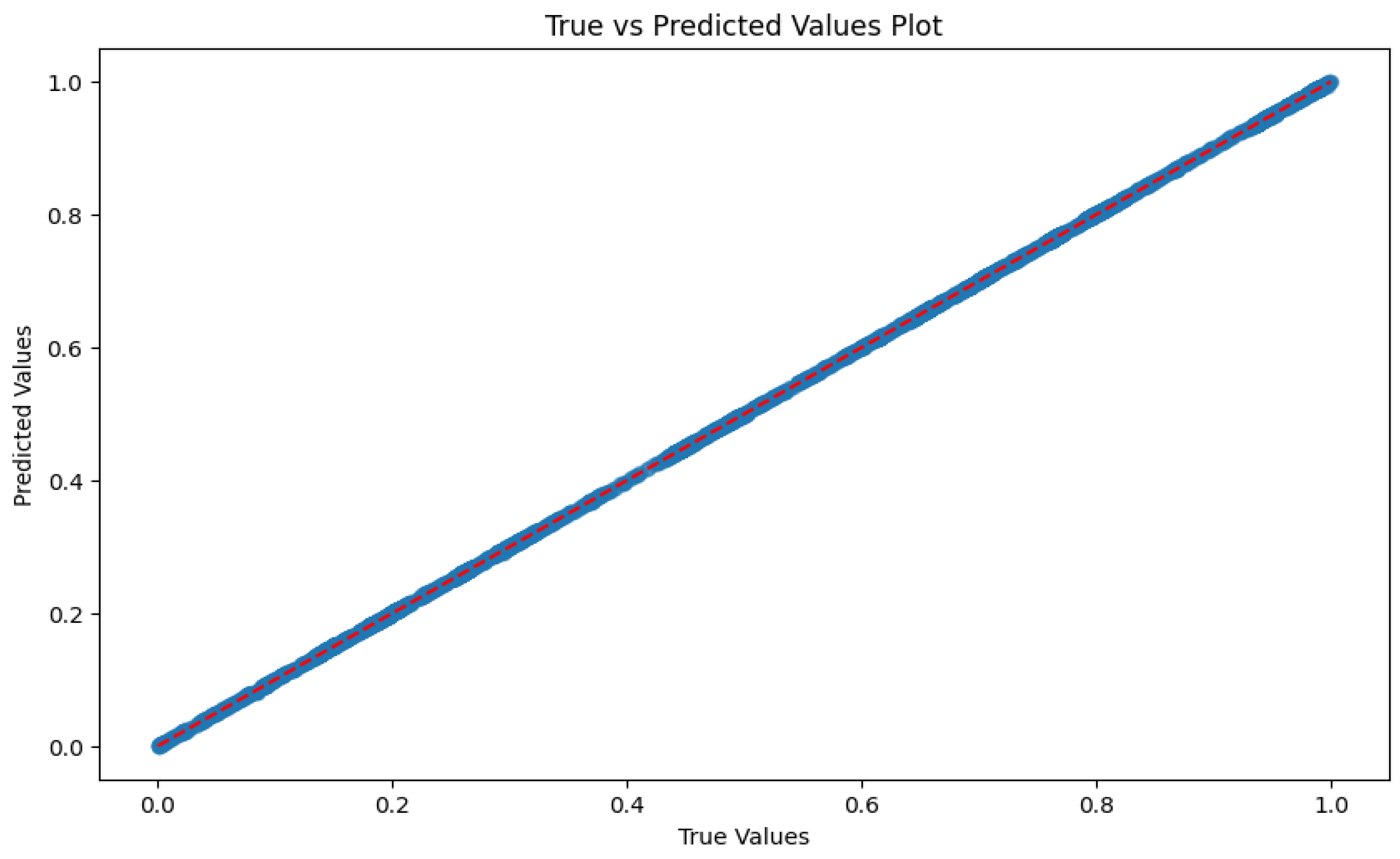
3.2.4. Real vs. Predicted Values

Figure 10 compares actual SoC values against predictions.

• X-Axis (True Values): this axis represents actual SoC values (%).
• Y-Axis (Predicted Values): this axis represents model-predicted SoC (%).
• Red Dotted Line (y = x): this line represents perfect agreement.
• Dispersion Points: the tight clustering of points around the red line is evident.

The tight clustering of predicted values around the red reference line indicates excellent alignment with actual SoC values, showcasing the model’s high predictive accuracy and reliability. This strong agreement confirms the model’s effectiveness in estimating SoC with precision.

3.2.5. Comparison of Results with Existing Models

As illustrated in

Table 5. Performance metrics (RMSE, MAE, MSE, and R²) for our model and baseline models.

Model/Work	MAE (%)	MSE (%)	R2	Cell Type Tested
Proposed LSTM model	0.43	0.23	0.99	LG 18650HG2
Obuli et al. (GPR) [38]	-	0.60	-	LG 18650HG2
Sadiqa et al. (ETR) [39]	0.09	0.39	0.99	LG 18650HG2
Sreekumar and Lekshmi (XGBoost) [40]	0.68	0.01	0.99	LG 18650HG2
RamParakash and Sivraj (GRU) [41]	0.90	-	-	US06, eVTOL, BMW i3
Hannan et al. (Transformer) [42]	0.44	-	0.99	LG 18650HG2

, compared to existing SOC estimation models such as Obuli et al. [38], Sadiqa et al. [39], Sreekumar and Lekshmi [40], RamParakash and Sivraj [41], and Hannan et al. [42], our proposed LSTM-based SOC estimation framework demonstrates competitive performance across key metrics.

Our model meets and exceeds the performance of many contemporary approaches, establishing it as a leading solution in SoC estimation.

4. Conclusions

This study successfully developed a robust deep learning model for the accurate prediction of batteries’ SoC, supported by an intuitive user interface for real-time applications. The model demonstrated excellent predictive accuracy through rigorous training, evaluation, and advanced hyperparameter tuning, as evidenced by its low error metrics and consistent performance across various tests. Integrating visual tools, such as the SoC tape, further enhanced user interaction by providing immediate and clear feedback.

The model achieved a Mean Squared Error (MSE) of 0.0023 in absolute value or 0.23% in percentage and a Mean Absolute Error (MAE) of 0.0043 in absolute value or 0.43% in percentage on the test dataset, showcasing its precision in estimating SoC. Regression analysis revealed a strong correlation between predicted and actual SoC values, with data points closely aligned along the regression line, and a high R² score of 0.99, indicating that the model accurately explains the variance in the data. Learning curves demonstrated rapid convergence and a low test loss of 1.12 × 10⁻⁶, affirming the model’s ability to generalize well to unseen data without overfitting. Residual analysis confirmed unbiased performance with consistent error distribution across all SoC ranges.

Key analyses, including regression, residual, and learning curves, highlighted the model’s reliability and robustness, with minimal bias and strong generalization capabilities. Additionally, this research underscored the potential for extending such predictive models to critical applications in EVs or renewable energies, where efficient battery management is vital for safety, reliability, and longevity.

This work advances battery monitoring systems and sets the stage for future developments, including exploring non-linear relationships, incorporating more complex neural network architectures, and applying them to diverse real-world conditions. These enhancements further strengthen the utility and adaptability of predictive models in energy management systems, such as energy-saving.

References

- Das, P.K. Battery Management in Electric Vehicles—Current Status and Future Trends. Batteries 2024, 10, 174. [Google Scholar] [CrossRef]
- Ghani, F.; An, K.; Lee, D. A Review on Design Parameters for the Full-Cell Lithium-Ion Batteries. Batteries 2024, 10, 340. [Google Scholar] [CrossRef]
- Adnan, M. The Future of Energy Storage: Advancements and Roadmaps for Lithium-Ion Batteries. Int. J. Mol. Sci. 2023, 24, 7457. [Google Scholar] [CrossRef] [PubMed]
- Lundberg, S.; Lee, S.-I. A Unified Approach to Interpreting Model Predictions. arXiv 2017, arXiv:1705.07874. [Google Scholar] [CrossRef]
- Xu, K.; Ba, J.L.; Kiros, R.; Cho, K.; Courville, A.; Salakhutdinov, R.; Zemel, R.S.; Bengio, Y. Show, Attend and Tell: Neural Image Caption Generation with Visual Attention. In Proceedings of the ICML’15: Proceedings of the 32nd International Conference on Machine Learning, Lille, France, 6–11 July 2015; pp. 2048–2055. Available online: https://arxiv.org/abs/1502.03044 (accessed on 29 January 2025).
- Meng, D.; Weng, J.; Wang, J. Experimental Investigation on Thermal Runaway of Lithium-Ion Batteries under Low Pressure and Low Temperature. Batteries 2024, 10, 243. [Google Scholar] [CrossRef]
- Sorensen, A.; Utgikar, V.; Belt, J. A Study of Thermal Runaway Mechanisms in Lithium-Ion Batteries and Predictive Numerical Modeling Techniques. Batteries 2024, 10, 116. [Google Scholar] [CrossRef]
- Sorouri, H.; Oshnoei, A.; Che, Y.; Teodorescu, R. A Comprehensive Review of Hybrid Battery State of Charge Estimation: Exploring Physics-Aware AI-Based Approaches. J. Energy Storage 2024, 100, 113604. [Google Scholar] [CrossRef]
- Zhao, F.; Guo, Y.; Chen, B. A Review of Lithium-Ion Battery State of Charge Estimation Methods Based on Machine Learning. World Electr. Veh. J. 2024, 15, 131. [Google Scholar] [CrossRef]
- Movassagh, K.; Raihan, A.; Balasingam, B.; Pattipati, K. A Critical Look at Coulomb Counting Approach for State of Charge Estimation in Batteries. Energies 2021, 14, 4074. [Google Scholar] [CrossRef]
- Errifai, N.; Rachid, A.; Khamlichi, S.; Saidi, E.; Mortabit, I.; El Fadil, H.; Abbou, A. Combined Coulomb-Counting and Open-Circuit Voltage Methods for State of Charge Estimation of Li-Ion Batteries. In Automatic Control and Emerging Technologies; ACET 2023; Lecture Notes in Electrical Engineering; El Fadil, H., Zhang, W., Eds.; Springer: Singapore, 2024; Volume 1141. [Google Scholar] [CrossRef]
- Bonfitto, A.; Feraco, S.; Tonoli, A.; Amati, N.; Monti, F. Estimation Accuracy and Computational Cost Analysis of Artificial Neural Networks for State of Charge Estimation in Lithium Batteries. Batteries 2019, 5, 47. [Google Scholar] [CrossRef]
- Zhang, D.; Zhong, C.; Xu, P.; Tian, Y. Deep Learning in the State of Charge Estimation for Li-Ion Batteries of Electric Vehicles: A Review. Machines 2022, 10, 912. [Google Scholar] [CrossRef]
- Lin, C.; Xu, J.; Jiang, D.; Hou, J.; Liang, Y.; Zou, Z.; Mei, X. Multi-Model Ensemble Learning for Battery State-of-Health Estimation: Recent Advances and Perspectives. J. Energy Chem. 2025, 100, 739–759. [Google Scholar] [CrossRef]
- Lehmam, O.; El Fallah, S.; Kharbach, J.; Rezzouk, A.; Ouazzani Jamil, M. State of Charge Estimation of Lithium-Ion Batteries Using Extended Kalman Filter and Multi-Layer Perceptron Neural Network. In Artificial Intelligence and Industrial Applications; Springer: Cham, Switzerland, 2023; pp. 59–72. [Google Scholar] [CrossRef]
- Tamilselvi, S.; Gunasundari, S.; Karuppiah, N.; Razak RK, A.; Madhusudan, S.; Nagarajan, V.M.; Sathish, T.; Shamim, M.Z.M.; Saleel, C.A.; Afzal, A. A Review on Battery Modelling Techniques. Sustainability 2021, 13, 10042. [Google Scholar] [CrossRef]
- Graham, J.; Wade, W. Reducing Greenhouse Emissions from Light-Duty Vehicles: Supply-Chain and Cost-Effectiveness Analyses Suggest a Near-Term Role for Hybrids. SAE J. STEEP 2024, 5, 151–168. [Google Scholar] [CrossRef]
- Rudner, T.G.J.; Toner, H. Key Concepts in AI Safety: Interpretability in Machine Learning. CSET Issue Brief 2021, 1–8. [Google Scholar] [CrossRef]
- Benallal, A.; Cheggaga, N.; Ilinca, A.; Tchoketch-Kebir, S.; Ait Hammouda, C.; Barka, N. Bayesian Inference-Based Energy Management Strategy for Techno-Economic Optimization of a Hybrid Microgrid. Energies 2024, 17, 114. [Google Scholar] [CrossRef]
- Pau, D.P.; Aniballi, A. Tiny Machine Learning Battery State-of-Charge Estimation Hardware Accelerated. Appl. Sci. 2024, 14, 6240. [Google Scholar] [CrossRef]
- Giazitzis, S.; Sakwa, M.; Leva, S.; Ogliari, E.; Badha, S.; Rosetti, F. A Case Study of a Tiny Machine Learning Application for Battery State-of-Charge Estimation. Electronics 2024, 13, 1964. [Google Scholar] [CrossRef]
- Bin Kaleem, M.; Zhou, Y.; Jiang, F.; Liu, Z.; Li, H. Fault detection for Li-ion batteries of electric vehicles with segmented regression method. Sci. Rep. 2024, 14, 31922. [Google Scholar] [CrossRef]
- Omojola, A.F.; Ilabija, C.O.; Onyeka, C.I.; Ishiwu, J.I.; Olaleye, T.G.; Ozoemena, I.J.; Nzereogu, P.U. Artificial Intelligence-Driven Strategies for Advancing Lithium-Ion Battery Performance and Safety. Int. J. Adv. Eng. Manag. 2024, 6, 452–484. [Google Scholar] [CrossRef]
- Liu, S.; Zhang, G.; Wang, C. Challenges and Innovations of Lithium-Ion Battery Thermal Management Under Extreme Conditions: A Review. ASME. J. Heat Mass Transfer. 2023, 145, 080801. [Google Scholar] [CrossRef]
- Ortiz, Y.; Arévalo, P.; Peña, D.; Jurado, F. Recent Advances in Thermal Management Strategies for Lithium-Ion Batteries: A Comprehensive Review. Batteries 2024, 10, 83. [Google Scholar] [CrossRef]
- Llamas-Orozco, J.A.; Meng, F.; Walker, G.S.; Abdul-Manan, A.F.N.; MacLean, H.L.; Posen, I.D.; McKechnie, J. Estimating the environmental impacts of global lithium-ion battery supply chain: A temporal, geographical, and technological perspective. PNAS Nexus 2023, 2, pgad361. [Google Scholar] [CrossRef]
- Machín, A.; Morant, C.; Márquez, F. Advancements and Challenges in Solid-State Battery Technology: An In-Depth Review of Solid Electrolytes and Anode Innovations. Batteries 2024, 10, 29. [Google Scholar] [CrossRef]
- Sarker, I.H. Machine Learning: Algorithms, Real-World Applications and Research Directions. SN Comput. Sci. 2021, 2, 160. [Google Scholar] [CrossRef]
- Kollmeyer, P.; Vidal, C.; Naguib, M.; Skells, M. LG 18650HG2 Li-ion Battery Data and Example Deep Neural Network xEV SOC Estimator Script. Mendeley Data 2020. [Google Scholar] [CrossRef]
- Editorial Team. LG HG2 Battery Review 18650 Test 20A 3000mAh Part 1. Batteries18650.com. 2016. Available online: https://www.batteries18650.com/2016/05/lg-hg2-review-18650-battery-test.html (accessed on 2 March 2025).
- Goumopoulos, C. A High Precision, Wireless Temperature Measurement System for Pervasive Computing Applications. Sensors 2018, 18, 3445. [Google Scholar] [CrossRef]
- Taye, M.M. Theoretical Understanding of Convolutional Neural Network: Concepts, Architectures, Applications, Future Directions. Computation 2023, 11, 52. [Google Scholar] [CrossRef]
- Cheggaga, N.; Benallal, A.; Tchoketch Kebir, S. A New Neural Networks Approach Used to Improve Wind Speed Time Series Forecasting. Alger. J. Renew. Energy Sustain. Dev. 2021, 3, 151–156. [Google Scholar] [CrossRef]
- Cervellieri, A. A Feed-Forward Back-Propagation Neural Network Approach for Integration of Electric Vehicles into Vehicle-to-Grid (V2G) to Predict State of Charge for Lithium-Ion Batteries. Energies 2024, 17, 6107. [Google Scholar] [CrossRef]
- Khalid, A.; Sundararajan, A.; Acharya, I.; Sarwat, A.I. Prediction of Li-Ion Battery State of Charge Using Multilayer Perceptron and Long Short-Term Memory Models. In Proceedings of the 2019 IEEE Transportation Electrification Conference and Expo (ITEC), Detroit, MI, USA, 19–21 June 2019; pp. 1–6. [Google Scholar] [CrossRef]
- Zhou, Y.; Wang, S.; Xie, Y.; Feng, R.; Fernandez, C. An Enhanced Bidirectional Long Short Term Memory-Multilayer Perceptron Hybrid Model for Lithium-Ion Battery State of Charge Estimation at Multi-Temperature Ranges. 2024. [CrossRef]
- Yalçın, O.G. Convolutional Neural Networks. In Applied Neural Networks with TensorFlow 2; Apress: Berkeley, CA, USA, 2021. [Google Scholar] [CrossRef]
- Babu, P.S.; Indragandhi, V.; Vedhanayaki, S. Enhanced SOC estimation of lithium ion batteries with RealTime data using machine learning algorithms. Sci. Rep. 2024, 14, 16036. [Google Scholar] [CrossRef]
- Jafari, S.; Byun, Y.C. Efficient state of charge estimation in electric vehicles batteries based on the extra tree regressor: A data-driven approach. Heliyon 2024, 10, e25949. [Google Scholar] [CrossRef] [PubMed]
- Sreekumar, A.V.; Lekshmi, R.R. Comparative Study of Data Driven Methods for State of Charge Estimation of Li-ion Battery. In Proceedings of the 2023 2nd International Conference on Paradigm Shifts in Communications Embedded Systems, Machine Learning and Signal Processing (PCEMS), Nagpur, India, 5–6 April 2023; pp. 1–6. [Google Scholar] [CrossRef]
- RamPrakash, S.; Sivraj, P. Performance Comparison of FCN, LSTM and GRU for State of Charge Estimation. In Proceedings of the 2022 3rd International Conference on Smart Electronics and Communication (ICOSEC), Trichy, India, 20–22 October 2022; pp. 47–52. [Google Scholar] [CrossRef]
- Hannan, M.A.; How, D.N.T.; Lipu, M.S.H.; Mansor, M.; Ker, P.J.; Dong, Z.Y.; Sahari, K.S.M.; Tiong, S.K.; Muttaqi, K.M.; Mahlia, T.M.I.; et al. Deep learning approach towards accurate state of charge estimation for lithium-ion batteries using self-supervised transformer model. Sci. Rep. 2021, 11, 19541. [Google Scholar] [CrossRef]