Utilizing Probabilistic Maps and Unscented-Kalman-Filtering-Based Sensor Fusion for Real-Time Monte Carlo Localization

Abstract

An autonomous car must know where it is with high precision in order to maneuver safely and reliably in both urban and highway environments. Thus, in this paper, a reliable and relatively precise position estimation (localization) technique for autonomous vehicles is proposed and implemented. In dealing with the obtained sensory data or given knowledge about the vehicle’s surroundings, the proposed method takes a probabilistic approach. In this approach, the involved probability densities are expressed by keeping a collection of samples selected at random from them (Monte Carlo simulation). Consequently, this Monte Carlo sampling allows the resultant position estimates to be represented with any arbitrary distribution, not only a Gaussian one. The selected technique to implement this Monte-Carlo-based localization is Bayesian filtering with particle-based density representations (i.e., particle filters). The employed particle filter receives the surrounding object ranges from a carefully tuned Unscented Kalman Filter (UKF) that is used to fuse radar and lidar sensory readings. The sensory readings are used to detect pole-like static objects in the egocar’s surroundings and compare them to the ones that exist in a supplied detailed reference map that contains pole-like landmarks that are produced offline and extracted from a 3D lidar scan. Comprehensive simulation tests were conducted to evaluate the outcome of the proposed technique in both lateral and longitudinal localization. The results show that the proposed technique outperforms the other techniques in terms of smaller lateral and longitudinal mean position errors.

1. Introduction

The technological challenges that need to be solved to attain complete autonomy are divided into four areas by designers and researchers in the autonomous driving field: perception, localization, path planning, and controls [1]. Perception is concerned with the task of detecting where objects like cars [2], trucks [3], bikes [4], and pedestrians are [5]; which lane the egocar is driving in [6]; where its boundaries are [7]; and so on. The solutions to these perception subtasks are researched using machine learning techniques that co-ordinate various sensors to accurately detect the surroundings of the egocar [8]. Sonar, radar, lidar, cameras, and other sensors are among them [9]. Further, there is also an additional layer of complexity here: certain objects do not move (static elements), while others do (dynamic elements), and it is critical to distinguish between the two [10].

On the other hand, localization is a vital function for self-driving cars [11], allowing them to locate their position within centimeters on a reference map [12]. This high degree of precision is necessary and allows a self-driving car to comprehend its surroundings and form an understanding of the road itself, road objects, and lane structures [13].

Additionally, the path-planning task is concerned with how an autonomous car drives from one point on the map (the initial position for the trip) to the final goal (the final position for the trip) [14]. It is divided into two subtasks: global path planning, which is the high-level path on the map for the desired trip, and local path planning, which generates a trajectory profile and a velocity profile for the egocar to maneuver across its environment while avoiding any obstacles, changing lanes, passing other vehicles, etc. The path-planning module receives information from both the perception and the localization modules and sends its generated trajectory to the control module [15].

Moreover, the controls task in autonomous cars is concerned with the automatic application of force on the car actuators to achieve the reference-trajectory tracking goals [16]. In self-driving cars, the controllers’ output is exerted on three actuators: steering, throttle, and brake systems [17]. The input information to these controllers takes several forms: the reference trajectory received from the egocar path-planning module, the egocar speed and acceleration signals, and the speed and acceleration of the preceding car [18].

This paper mainly focuses on localization and how to improve its accuracy, as it allows the autonomous car to better comprehend its surroundings and form an understanding of the road and lane structures (e.g., when a lane forks or merges, schedule lane changes and determine lane routes even when markers are obscured) [19].

Sensors play a key role in autonomous vehicle localization, with vehicles being typically equipped with a combination of GPS, IMU, cameras, lidar, radar, and odometry sensors. These sensors provide data about the vehicle’s surroundings and its own motion, forming the foundation for accurate localization. Sensor fusion is a crucial technique that integrates data from multiple sensors to enhance accuracy and reliability. By combining information from sources like GPS, IMU, and lidar, a vehicle can compensate for the limitations of individual sensors, improving overall localization performance. Odometry is another important component estimating the vehicle’s position based on changes in motion, such as wheel speed and steering angle. While useful, odometry tends to accumulate errors over time, prompting its use in conjunction with other localization methods. Map matching involves comparing sensor data with pre-existing maps of the environment, aiding in the identification of the vehicle’s location. This technique is particularly beneficial in environments with recognizable landmarks, contributing to precise localization. Particle filters, a probabilistic method, maintain a set of potential vehicle poses based on sensor measurements and motion models. As the vehicle moves, this set of poses is updated to converge toward the most likely position, enhancing the accuracy of localization.

The 3D pose of an autonomous car inside a high-definition (HD) map, comprising 3D location, 3D orientation, and associated uncertainty, is provided using localization [20]. Unlike the usage of a navigation map with GPS, which only requires a few meters of precision, the localization of a self-driving car requires a far greater level of accuracy relative to the map, generally in the range of centimeters and a few tenths of degree [20].

A landmark-based reference map represents a balanced approach between no-map (SLAM) techniques and detailed high-definition mapping techniques and is thus adopted in this study. Moreover, as a contribution, this work does not depend on a single sensor (lidar), with its high resolution but well-known limitations (e.g., limited reach; severely affected by fog, snow, or dust [21]), but fuses it with radar (e.g., long reach, not affected by fog, but with low resolution [22]) to strengthen both methods and obtain the best out of them. Additionally, by using a carefully tailored UKF as the employed fusion technique, pole-like landmarks can be detected with greater precision and robustness. As an additional contribution, this paper addresses the uncertainties in the detected pole-like landmark co-ordinates. They are represented on the reference map in a probabilistic form. This allows Bayesian inference, applied using a tailored version of a particle filter, to estimate the egocar pose.

2. Literature Review

Satellite-based localization has been available for decades and has undergone various upgrades. Newer systems, such as RTK-GPS [23] or DGPS [24], provide efficient options since they attain centimeter-level precision without the use of any extra techniques. Nonetheless, there are significant uncertainties concerning their consistency. Structures or other towering road obstacles that obscure the line of sight between the car and the satellites can reduce precision by some meters [25] in metropolitan areas [26]. Moreover, the latency for acquiring the signals usually comes with errors, which is a critical issue that needs to be addressed [27] by filtration, noise cancelation, and compensating for missing readings [28].

As an alternative to the RTK-GPS and according to [15], lidar approaches were shown to be the most promising in terms of performance for the localization of self-driving vehicle applications. Nevertheless, they demand high processing and computational power, in addition to their high cost. Thus, they are rendered to be impracticable in terms of commercialization and cost-affordability. Therefore, greater lidar technology enhancement or alternative methodologies like vision-based localization or ground-penetrating radar localization within lidar maps may open the door for more feasible systems from a commercial point of view. Nevertheless, before these systems can be mass-deployed, further study will be needed to evaluate their robustness, validate their performance across a range of driving circumstances, and refine operation settings.

Accordingly, using reference-dense maps [20] could provide a more reliable localization option [29]. These maps may take several forms like point clouds [30], grid maps [31], or polygon meshes [32]. Nevertheless, map-based systems have the fundamental disadvantage of requiring a substantial amount of memory, which quickly becomes pricey when larger-scale maps are employed [33]. To address this issue, “landmark maps” have sparked significant attention [11]. These maps contain only a very limited number of recognizable and designated features that have been extracted from huge volumes of raw sensory data (collected from cameras, radars, and lidars) and condensed [34], which, in return, reduces the needed memory use by several orders of magnitude.

Subsequently, several efforts have been made in recent research to tackle the challenge of car localization by the employment of lidar point clouds from which pole-like markers are identified. This issue is separated into two sub-problems. The first sub-problem is concerned with the detection of poles and the estimation of their positions, while the second one is concerned with the estimation of the egocar pose based on the position of the detected poles. For example, a pole detector is created by Weng et al. [35] by dividing the region around the egocar and counting the reflected-scan points in each voxel. The detection of poles is accomplished by recognizing the stacks of voxels that are vertically linked and all surpass a predefined threshold. Additionally, the detector employs the RANSAC algorithm [36] to fit all of the points associated with the discovered stacks of voxels to a cylindrical shape. When it comes to the egocar pose estimation, the nearest-neighborhood data association is utilized and paired with a particle filter.

Furthermore, the main emphasis of the Sefati et al. pole-detection approach is to eliminate the ground plane from the point cloud generated by the sensors [37]. A horizontal regular grid is then constructed from the projection of the remaining point-cloud points. The occupancy and height parameters are used to cluster the neighboring cells, and a cylinder is fitted to each of the resulting clusters. Similarly, for the egocar pose estimation, the nearest-neighborhood data association is also employed and paired with a particle filter.

Kummerle et al. improved on the previous work by fitting planes to point-cloud-constructed building facades and also fitting lines to lane markings extracted from stereo camera images [34]. The previous improvements enhance the pole detection, which consequently improves the pose estimation by employing a Monte Carlo method to tackle the data association stage and a nonlinear least-squares optimization technique to refine the finally computed pose.

A more comprehensive work was conducted by Schaefer et al. [38] as they propose three phases to construct a full localization system based on landmark detection. The first phase is the pole extractor, the second one is the mapping, and the third one is the localization. The method used for pole detection considers both the endpoint of the laser beams as well as the available open space between the lidar and those beam endpoints. Therefore, based on a map of only pole landmarks, the presented method demonstrates precise and consistent car localization for large time scales. Experiments are carried out for 35 hours over the course of 15 months going through different circumstances like construction zones, weather and seasonal variations, different routes, and hordes of moving objects.

Several attempts have been made to remove the dependency on reference maps and only depend on the mounted sensors on the egocar. These endeavors focus on constructing a map and computing localization simultaneously in what is called simultaneous localization and mapping (SLAM) techniques [39]. However, these techniques are computationally much more expensive than the ones that depend on reference maps. Therefore, they usually rely on approximations to speed up processing and create a functional outcome [40]. Consequently, the lack of precision in these techniques hinders their applicability to autonomous driving.

The research gap addressed by this paper lies in the need for a nuanced and versatile mapping technique that strikes a balance between simultaneous localization and mapping (SLAM) methods, which lack mapping information, and high-definition mapping techniques, which can be overly detailed. In contrast to existing approaches, this work adopts a landmark-based reference map, providing a more comprehensive mapping solution.

Furthermore, the existing literature often relies on a single high-resolution sensor, such as lidar, which, despite its advantages, has well-known limitations, including restricted reach and vulnerability to environmental factors like fog, snow, or dust. This paper contributes by adopting a fusion approach, combining lidar with radar. While radar offers a longer reach and is less affected by adverse weather conditions, it has lower resolution. The integration of these complementary sensors is designed to capitalize on their individual strengths and mitigate their weaknesses.

Additionally, the paper introduces a carefully tailored Unscented Kalman Filter (UKF) as the fusion technique, enhancing precision and robustness in detecting pole-like landmarks. This aspect represents a research gap in sensor fusion techniques for landmark-based mapping.

Moreover, the paper addresses a crucial research gap by acknowledging and handling uncertainties in the detected pole-like landmark co-ordinates. Unlike existing methods, this study represents uncertainties in a probabilistic form on the reference map, enabling Bayesian inference. The application of a tailored particle filter allows for the estimation of egocar pose while considering uncertainties, contributing to the overall robustness and reliability of the localization system. This unique approach to handling uncertainties in landmark-based mapping represents a novel contribution to the existing body of research in autonomous vehicle localization.

3. Overview of the Proposed Localization Algorithm

This work proposes a Real-Time Monte Carlo Localization (RTMCL) algorithm for driverless vehicles. The details and the workflow of this algorithm are shown below in Figure 1.

The information required as input by the RTMCL algorithm can be categorized into four groups as follows:

(1)

Global position information: this information mainly comes from the GPS. If an IMU unit is also installed in the egocar, then a fusion between the GPS and IMU signals is implemented, resulting in a single output (initial egocar pose) that is used at a later stage by the particle filter. The fusion helps to correct errors that accumulate out of the dead reckoning [41] in periods with missing GPS position deliveries.

(2)

Odometry measurements: the algorithm requires the readings of the egocar speed and the steering angle (to calculate the yaw rate). Both will be used to update the particle filter state after filtering from high noise.

(3)

Object-detection sensory output: these are mainly lidar, radar, and camera data. Since the camera is not used in this work, only radar and lidar data are collected and fused using the tailored UKF, whose output is clustered using the GB-DBSCAN algorithm to detect potential pole-like static objects. The velocity measurements (the Doppler signal) received from the radar will help screen out dynamic objects.

(4)

Reference landmarks map: this map must be developed in a way to contain pole-like landmarks with full co-ordinates, which will be extracted in an offline process from 3D point-cloud lidar data. The map pole-like landmarks will be aligned with the detected pole-like landmarks (by GB-DBSCAN) through the “data association” process. The Iterative Closest Point (ICP) technique is employed to perform this “data association”, which is a very critical step to achieving accurate localization [42].

The above categories of input signals are used by the tailored PF (which will be presented later in more detail [43]) to search for the most accurate egocar pose. The PF is initialized using the output signal of the GPS and IMU fusion and produces a much more precise pose with the help of the identified pole-like landmarks and the reference map.

4. Overview of the UKF

The KF is an equation-based system that works as a predictor–update cyclic optimum estimator that minimizes the estimated error covariance [44]. Given the measurement $z\in R^m$ of a discrete-time-controlled process described by a set of linear stochastic difference equations, the Kalman filter predicts the state $x\in R^n$.

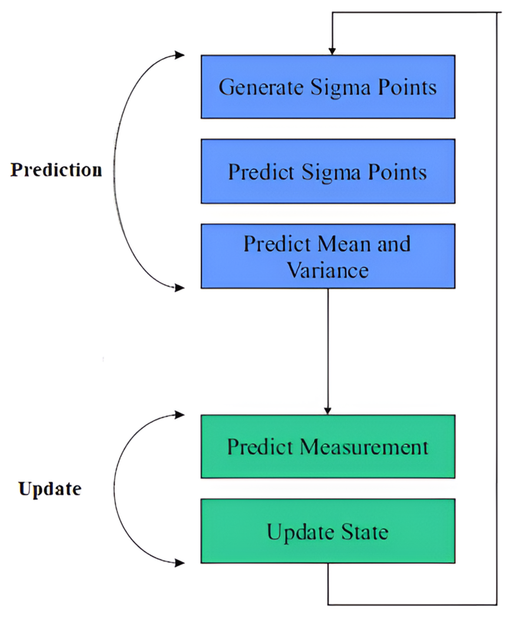
Inapplicably, because KF is restricted to linear processes, it is incompatible with the radar measurement process, which is fundamentally nonlinear. To solve this restriction, the UKF was developed [45]. The UKF is a deterministic sampling-based derivative-free alternative to the extended Kalman filter [46]. The UKF also employs the predict–update two-step procedure, but it has been supplemented with additional processes such as sigma point production and prediction, as presented in Figure 2.

The state Gaussian distribution is represented in the UKF process by a small number of wisely picked sample points known as sigma points. The $n_x=2n+1$ sigma points are chosen using the following formula:

$$X_k=\left[x_k x_k+\sqrt{\left(\lambda +n_x\right)P_k} x_k-\sqrt{\left(\lambda +n_x\right)P_k}\right]$$

(1)

where $P_k$ is the Kalman filter process estimate covariance matrix, $X_k$ is the sigma-point matrix containing $n_x$ sigma-point vectors, and $\lambda$ is a design parameter that defines the spread of the produced sigma points and often is calculated as $\lambda =3-n_x$.

Each produced sigma point is entered into the UKF nonlinear process model described in Equation (2) to build the matrix of predicted sigma points $\widehat{X}$ with an $n\times n_x$ dimension in what is called the sigma-point prediction phase.

$${\widehat{X}}_{k+1}=f\left(X_k, {\nu }_k\right)$$

(2)

where ${\nu }_k$ is the white noise of the process, which is modeled as a Gaussian distribution ($\mathcal{N}$) with zero mean and covariance matrix $Q_k$.

The mean and covariance matrices of the predicted state are then computed from the projected sigma points using Equation (3):

$$\begin{gathered} {\widehat{x}}_{k+1}={\displaystyle \sum }_{i=0}^{n_x}{w}_i{\widehat{X}}_{k+1, i} \\ {\widehat{P}}_{k+1}={\sum }_{i=0}^{2n_x}{w}_i\left({\widehat{X}}_{k+1,i}-{\widehat{x}}_{k+1}\right){\left({\widehat{X}}_{k+1,i}-{\widehat{x}}_{k+1}\right)}^T \end{gathered}$$

(3)

where $w_i$ is the sigma-point weights that are applied to invert the sigma-point spreading. These weights are computed as follows in Equation (4):

$$\begin{gathered} w_i=\frac{\lambda }{\lambda +n_x}, i=0 \\ {w}_i=\frac{1}{2\left(\lambda +n_x\right)}, i=1\dots n_x \end{gathered}$$

(4)

Each produced sigma point is entered into the nonlinear UKF’s measurement model described by Equation (5) to build the matrix of predicted measurement sigma points with an $n\times n_x$ dimension in the measurement prediction phase.

$${\widehat{Z}}_{k+1}=h\left({\widehat{X}}_{k+1}\right)$$

(5)

The mean and covariance matrices of the predicted measurement are then computed using the predicted sigma points and the covariance matrix R of the measurement noise, as shown in Equation (6):

$$\begin{gathered} {\widehat{z}}_{k+1}={\sum }_{i=0}^{n_x}{w}_i{\widehat{Z}}_{k+1, i} \\ {S}_{k+1}={\sum }_{i=0}^{2n_x}{w}_i\left({\widehat{Z}}_{k+1,i}-{\widehat{z}}_{k+1}\right){\left({\widehat{Z}}_{k+1,i}-{\widehat{z}}_{k+1}\right)}^T+R \\ R=E\left\{{\omega }_k.{\omega }_k^T\right\} \end{gathered}$$

(6)

where $w_i$ is the sigma-point weights computed in Equation (4), $S_k$ is the measurement covariance matrix, and $E\left\{.\right\}$ Is the expected value of the measurement of white noise ${\omega }_k$, which is modeled as a Gaussian distribution ($\mathcal{N}$) with zero mean and covariance matrix $R.$

The final stage is the UKF state update, in which the gain matrix ($K$) of the UKF is produced using the estimated cross-correlation matrix ($T$) between the sigma points in the state space and the measurement space, as in Equation (7). The gain is applied to both the UKF state vector ($x$) and the state covariance matrix ($P$).

$$\begin{gathered} T_{k+1}={\displaystyle \sum }_{i=0}^{2n_x}{w}_i\left({\widehat{X}}_{k+1,i}-{\widehat{x}}_{k+1}\right){\left({\widehat{Z}}_{k+1,i}-{\widehat{z}}_{k+1}\right)}^T \\ {K}_{k+1}=T_{k+1}{S}_{k+1}^{-1} \\ {x}_{k+1}={\widehat{x}}_{k+1}+K_{k+1}\left({\widehat{z}}_{k+1}-z_{k+1}\right) \\ {P}_{k+1}={\widehat{P}}_{k+1}-K_{k+1}{S}_{k+1}{K}_{k+1}^T \end{gathered}$$

(7)

5. Model of the Road Object

A motion model for a road object in the context of autonomous vehicles typically describes how the object’s position and velocity evolve over time. The goal is to predict the future trajectory of the road object, enabling the autonomous vehicle to anticipate its movements and make informed decisions. Any object in the road is represented by five variables (state representation). These variables are grouped into one vector called the state vector $x$. Equation (8) presents $x$ with its variables $p_x$, $p_y$, $v$, $\psi$, and $\dot{\psi }$, which are the object location in the x and y axes, the magnitude of the object’s velocity calculated from its x and y components ($v_x$ and $v_y$), the yaw angle (object orientation), and the rate at which the object-yaw angle changes, respectively, as shown in Figure 3.

$$x=\left[\begin{array}{c}{p}_x\\ p_y\\ v\\ \psi \\ \dot{\psi }\end{array}\right], v=\sqrt{v_x^2+v_y^2},\psi =ta{n}^{-1}\frac{v_y}{v_x}$$

(8)

Based on the state vector $x$, the nonlinear $x_{k+1}=f\left(x_k,{\nu }_k\right)$ difference equation (dynamic equations) that represents the object’s motion model is constructed and provided in Equations (9)–(11).

$$x_{k+1}=x_k+\left[\begin{array}{c}\begin{array}{c}\frac{v_k}{{\dot{\psi }}_k}\left(sin\left({\psi }_k+{\dot{\psi }}_k\mathrm{\Delta }t\right)-sin\left({\psi }_k\right)\right)\\ \frac{v_k}{{\dot{\psi }}_k}\left(-cos\left({\psi }_k+{\dot{\psi }}_k\mathrm{\Delta }t\right)+cos\left({\psi }_k\right)\right)\\ 0\end{array}\\ \mathrm{\Delta }t\\ 0\end{array}\right]+{\nu }_k$$

(9)

$${\nu }_k=\left[\begin{array}{c}\begin{array}{c}\frac{1}{2}{\left(\mathrm{\Delta }t\right)}^{2}cos\left({\psi }_k\right).{\nu }_{a,k}\\ \frac{1}{2}{\left(\mathrm{\Delta }t\right)}^{2}sin\left({\psi }_k\right).{\nu }_{a,k}\\ \mathrm{\Delta }t.{\nu }_{a,k}\end{array}\\ \frac{1}{2}{\left(\mathrm{\Delta }t\right)}^2.{\nu }_{\ddot{\psi ,k}}\\ \mathrm{\Delta }t.{\nu }_{\ddot{\psi ,k}}\end{array}\right]$$

(10)

$$\begin{gathered} \mathrm{\Delta }t=t_{k+1}-t_k \\ {\nu }_{a,k}~\mathcal{N}\left(0, {\sigma }_a^2\right) \\ {\nu }_{\ddot{\psi },k}~\mathcal{N}\left(0, {\sigma }_{\ddot{\psi }}^2\right) \end{gathered}$$

(11)

where $\mathrm{\Delta }t$ is the time difference between two consecutive samples and is the longitudinal acceleration, ${\nu }_{\ddot{\psi },k}$ is the longitudinal acceleration noise (noise modeling) at sample k with a standard deviation of ${\sigma }_a^2$, and $\ddot{\psi }$ is the yaw acceleration noise at sample $k$ with a standard deviation of ${\sigma }_{\ddot{\psi }}^2$.

If the $\dot{\psi }$ is zero, and to avoid dividing by zero in Equation (9), the subsequent approximation is applied (linear model) to evaluate the prediction of $p_x$, and $p_y$:

$$\begin{gathered} p_{x_{k+1}}=p_{x_k}+v_{k}cos\left({\psi }_k\right)\mathrm{\Delta }t \\ {p}_{y_{k+1}}=p_{y_k}+v_{k}sin\left({\psi }_k\right)\mathrm{\Delta }t \end{gathered}$$

(12)

6. UKF-Based Lidar/Radar Fusion

The lidar measures the centroid of the object’s position (moving or stationary) in Cartesian co-ordinates ($p_x$ and $p_y$), as given by Equation (13), while the radar measures the same object’s centroid position in polar co-ordinates ($\rho$, $\phi$). Moreover, the radar also measures the object’s velocity ($\dot{\rho }$), as given by Equation (14). Therefore, to unify the way of measurement, a mapping function is used (in Equation (15)) to convert the lidar Cartesian co-ordinates to polar form.

$$z_{lidar}=\left(\begin{array}{c}{p}_x\\ p_y\end{array}\right), z_{radar}=\left(\begin{array}{c}\rho \\ \phi \\ \dot{\rho }\end{array}\right)$$

(13)

$$h\left(x\right)=\left(\begin{array}{c}\rho \\ \phi \\ \dot{\rho }\end{array}\right)=\left(\begin{array}{c}\sqrt{p_x^2+p_y^2}\\ arctan\left(\frac{p_y}{p_x}\right)\\ \frac{p_x{v}_x+p_y{v}_y}{\sqrt{p_x^2+p_y^2}}\end{array}\right)$$

(14)

$$p_x=\rho cos\left(\phi \right), p_y=\rho sin\left(\phi \right)$$

(15)

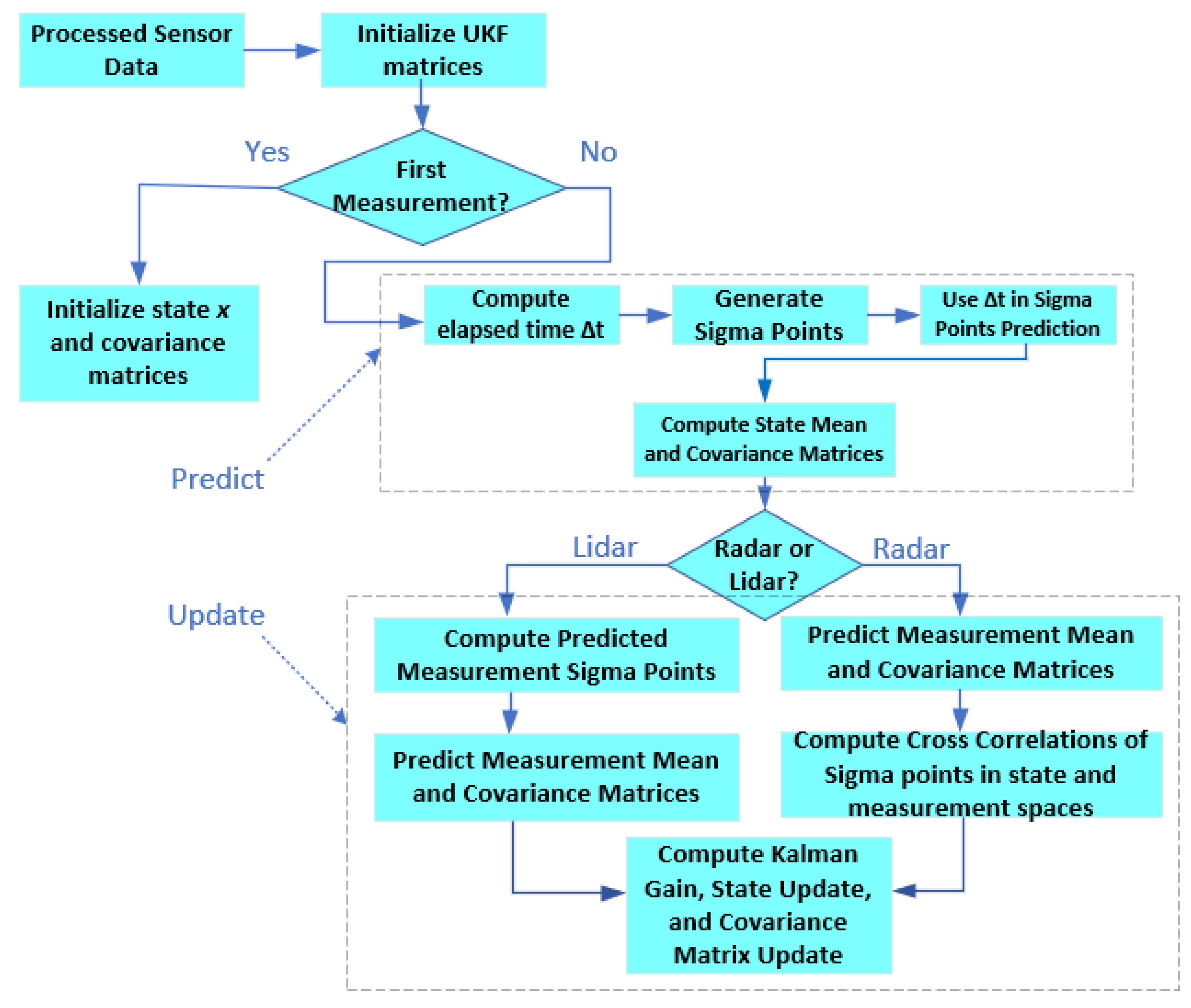
As shown in Figure 4, the prediction step is conducted for both lidar and radar simultaneously. However, the update step is specific for each sensor since each sensor has its own measurement model. Moreover, the update of the belief is executed upon the arrival of a new sensor measurement (both sensors are not synchronized).

After the initialization steps for both the UKF and the measurement models for both the lidar and radar, the time step ($\mathrm{\Delta }t$) is computed as shown in Figure 4 and, at the same time, using Equation (1), the sigma point ($X_k$) is created. The predicted sigma point (${\widehat{X}}_{k+1}$) for the next time step is calculated using Equation (2), utilizing the object’s model given by Equation (9). Then, the predicted state mean vector (${\widehat{x}}_{k+1}$) and its covariance matrix (${\widehat{P}}_{k+1}$) is calculated by applying Equation (3).

For the update step in the fusion process, there are two branches. The first one is the lidar branch and the second one is the radar branch. The last received measured signal will decide which branch the workflow will assume (either lidar or radar signal). If a radar signal is received, the predicted measurement sigma point (${\widehat{Z}}_{k+1}$) is computed based on the model in Equation (14) and from ${\widehat{X}}_{k+1}$ in Equation (5). Then, ${\widehat{z}}_{k+1}$ states that the covariance $S_{k+1}$ and the noise covariance $R_{radar}$ are computed based on Equation (6). The $R_{radar}$ covariance matrix is further defined as given in Equation (16) below:

$$R_{radar}=\left[\begin{array}{ccc}{\sigma }_{\rho }^2& 0& 0\\ 0& {\sigma }_{\phi }^2& 0\\ 0& 0& {\sigma }_{\dot{\rho }}^2\end{array}\right]$$

(16)

where ${\sigma }_{\dot{\rho }}$, ${\sigma }_{\phi }$, and ${\sigma }_{\rho }$ are the noise SD of the object yaw rate, the noise SD of the object heading, and the noise SD of the object radial distance, respectively.

The cross-correlation matrix ($T_{k+1}$) is then computed based on the resulting state vectors ${\widehat{x}}_{k+1}$ and ${\widehat{z}}_{k+1}$ with their counterparts ${\widehat{X}}_{k+1}$ and ${\widehat{Z}}_{k+1},$ respectively using Equation (7). The $T_{k+1}$ is then used to compute the UKF gain ($K_{k+1}$), which is consequently used to compute the updated state vector ($x_{k+1}$) and covariance matrix ($P_{k+1}$), as shown in Equation (7). Then, $x_{k+1}$ and $P_{k+1}$ will be used to generate the new sigma points ($X_{k+1}$) in the next iteration, etc.

Instead, if a lidar signal is received, the predicted measurement sigma point (${\widehat{Z}}_{k+1}$) is computed based on the linear lidar measurement model in Equation (17) and directly from ${\widehat{X}}_{k+1}$. Then, ${\widehat{z}}_{k+1}$ states that the covariance $S_{k+1}$ and the noise covariance $R_{lidar}$ are computed based on Equation (6) with more detail of $R_{lidar}$ in Equation (17).

$$\begin{gathered} H_{lidar}=\left[\begin{array}{ccccc}1& 0& 0& 0& 0\\ 0& 1& 0& 0& 0\end{array}\right] \\ {R}_{lidar}=E\left[\omega .{\omega }^T\right]=\left[\begin{array}{cc}{\sigma }_{p_x}^2& 0\\ 0& {\sigma }_{p_y}^2\end{array}\right] \end{gathered}$$

(17)

where the object $x$ and $y$ positions, ${\sigma }_{p_x}$ and ${\sigma }_{p_y}$, are the noise SDs, respectively. Likewise, the radar, the cross-correlation matrix ($T_{k+1}$), the KF gain ($K_{k+1}$), and the covariance matrix ($P_{k+1}$) are computed from Equation (7).

7. Point-Cloud Clustering and Association

The point cloud resulting from the application of the UKF fusion algorithm presented in Figure 4 offers details about the objects in the surroundings of the egocar. To extract each object’s information (geometrical shape and pose), clustering is employed on the UKF point cloud to characterize each object in a source-point model form, which will significantly lower the computation overhead and memory prerequisite.

The clustering in this work is performed using the GB-DBSCAN algorithm, which is a variation of the original DBSCAN algorithm [47], which is an unsupervised learning algorithm that arranges data points with high density together in one group. Two parameters are used to tune the DBSCAN algorithm and define the allowed density. “ε” is the first parameter to tune, which defines the allowed radial distance from the point under evaluation “p”. “minPts” is the second parameter that determines the lowest number of detection points that are located within a distance “ε” from “p”, including “p” itself, to form a cluster. Therefore, the determination of the density of points to be grouped together to form a cluster is conducted by the proper selection of “ε” and “minPts”. However, if the objects to be detected take several topologies (other than circular), as with the case of road objects, the DBSCAN algorithm is not enough. An improvement came from Dietmayer et al. [48] by proposing not to use fixed parameters like “ε” and “minPts” in the GB-DBSCAN but, instead, forming a polar grid taking into account the angular and radial resolution of the sensor. The search area is not necessarily a circular one with a fixed radius but can be a dynamic elliptic one. Therefore, this algorithm is very appropriate for pole-like objects, as their distinctive feature is that they produce a high density of detection points, much more than their surroundings.

The outcome of the GB-DBSCAN algorithm is a coarse clustering of the UKF fusion data. The application of the RANSAC algorithm fine-tunes these clusters and associates geometrical shape proposals with them [36]. For the pole-like landmarks, the most appropriate geometrical shape is the circular one, which is fitted to all the $N$ points in each cluster. The RANSAC algorithm then finds the parameters of each fitted circle (the radius ($\widehat{r}$) and the centroid (${\widehat{x}}_c,{\widehat{y}}_c$)), which will represent a pole landmark, by finding the optimal solution of the following formula:

$$\min \left\{\frac{1}{N}{\sum }_{i=1}^N{\left[\sqrt{{\left(x_i-{\widehat{x}}_c\right)}^2+{\left(y_i-{\widehat{y}}_c\right)}^2}-\widehat{r}\right]}^2\right\}$$

(18)

Once the pole-like landmarks are identified in the source UKF fusion data, the data association step takes place by linking these identified landmarks with their matched counterpart in the target (the supplied reference map). The employed PF relies heavily on precision in this step. The association is implemented using the ICP algorithm [42]. The standard ICP searches the whole point clouds in both the source and the target; however, here, only the centroids are considered during the objects’ matching process, which, in return, saves a significant amount of memory and processing overhead.

The ICP algorithm is composed of two phases that run iteratively till convergence is reached. In our case, we have a set X representing the source points (UKF data) and another set Y representing the target points (a point-cloud map). The first phase is the matching between each point in X with the closest point in Y. The second phase is to find the optimal transform (X→Y) given the matched association. Storing the X and Y sets in the form of a KD tree data structure [49] is very crucial for the efficient matching by distance performed by the ICP. $x_i$ and $y_i$ are two matched points from X and Y sets, respectively. The 2D ICP algorithm finds the rotation angle “$\phi$” and the translation parameter “t” that minimizes the summation of the quadratic distance between the target and the source points, as presented by Equation (19). Note that the rotation matrix $R\left(\phi \right)$ uses angle “$\phi$” as a variable.

$$mi{n}_{\phi ,t}\left\{{{\displaystyle \sum }}_{i=1}^N{\left(y_i-\left(R\left(\phi \right)x_i-t\right)\right)}^T\left(y_i-\left(R\left(\phi \right)x_i-t\right)\right)\right\}$$

(19)

The co-ordinate system must be unified between the egocar co-ordinates ($x_c$ and $y_c$) and the reference map co-ordinates ($x_m$ and $y_m$) to perform the data association correctly. Therefore, the homogenous transformation is used (in the form of a transformation matrix) as given by Equation (20). The translation and rotation are performed using map particle/egocar co-ordinates ($x_p$ and $y_p$) and the rotation angle $\theta$.

$$\left[\begin{array}{c}{x}_m\\ y_m\\ 1\end{array}\right]=\left[\begin{array}{ccc}cos\theta & -sin\theta & x_p\\ sin\theta & cos\theta & y_p\\ 0& 0& 1\end{array}\right]\times \left[\begin{array}{c}{x}_c\\ y_c\\ 1\end{array}\right]$$

(20)

8. Details of the Particle Filter

For a stochastic process that has noisy observations $p\left(z_t|x_t\right)$, the posterior distribution $bel\left(x_t\right)$ could be represented by a finite set of particles. This is considered an approximate implementation of the Bayesian filter in a recursive mode with a normalization factor $\zeta$ that is given by Equation (21):

$$bel\left(x_t\right)\leftarrow \zeta p\left(z_t|x_t\right) bel\left(x_{t-1}\right)$$

(21)

The higher the particles’ number $M$, the more accurate the representation of the belief distribution $bel\left(x_t\right)$, where t denotes the time step at which the state of the set of the particles is considered, as given by Equation (22):

$${\chi }_t=\left\{x_t^{\left[i\right]}|1\le i\le M\right\}$$

(22)

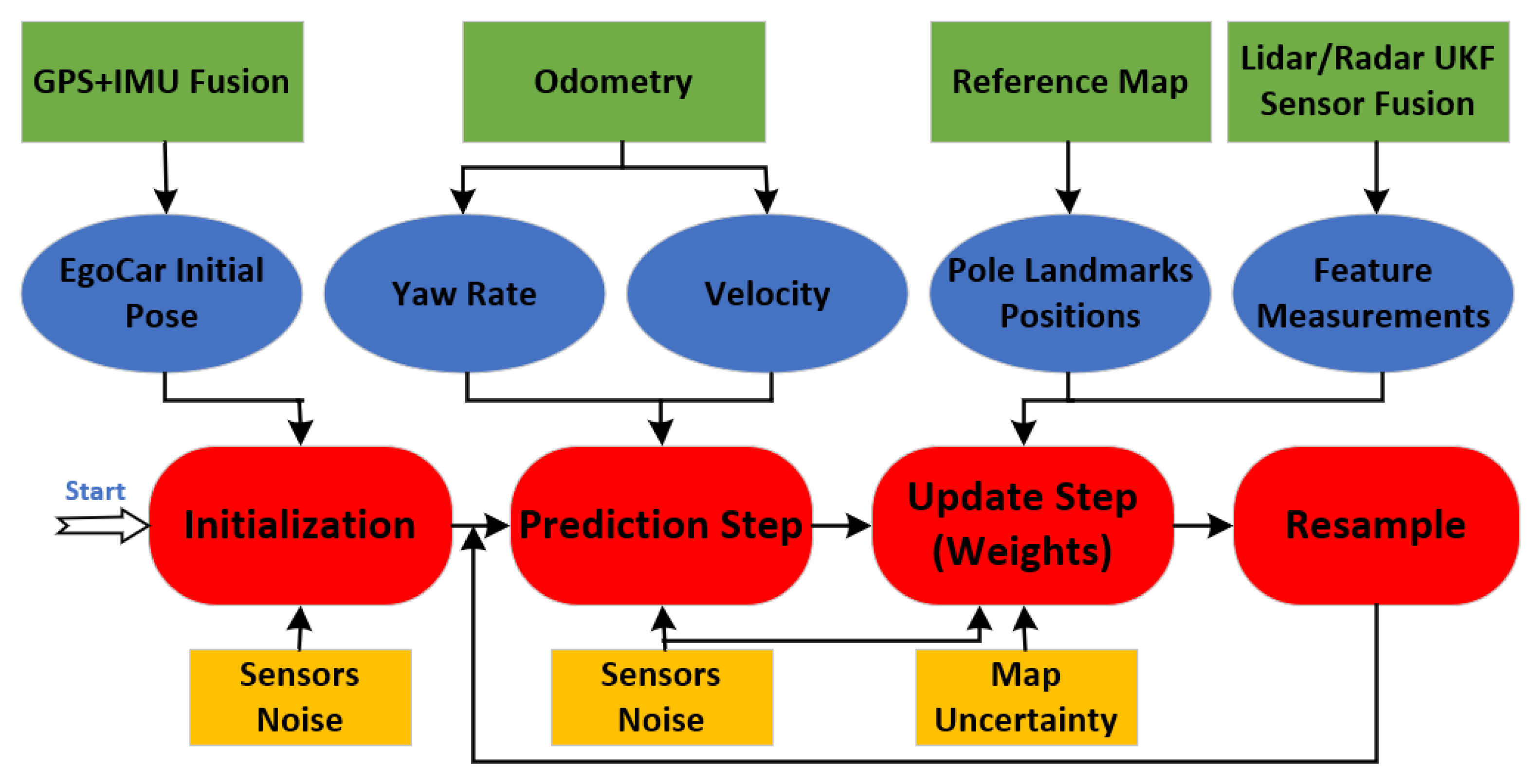
The actual state (the optimal solution) will be one of the particles included in the set ${\chi }_t$ at time t. Therefore, each $x_t^{\left[i\right]}$ represents a hypothesis for the optimal solution. The implementation of the employed PF in the work is presented in Algorithm 1. Moreover, the workflow of the PF is illustrated in Figure 5. Upon receipt of a new measurement (odometry) signal ($u_t$) or a pole-like object measurement update ($z_t$) from the UKF, a new search for an optimum egocar pose is initiated.

Algorithm 1. Workflow of the employed PF.

Procedure Particle Filter (${\chi }_{t-1}, u_t, z_t$):

Input: Set of particles ${\chi }_{t-1}$ at a time ($t-1$), control    inputs $u_t$, and a set of measurements $z_t$. Output: The updated set of particles ${\chi }_t$ at time $t$.

Begin Initialize Particles: ${\overline{\chi }}_t={\chi }_t=\varnothing$. $For m=1 to M do$ i. $generate x_i^{\left[m\right]}~p\left(x_t|u_t,x_{t-1}^{\left[m\right]}\right)$ ii. $w_t^{\left[m\right]}=p\left(z_t|x_i^{\left[m\right]}\right)$ iii. ${\overline{\chi }}_t={\overline{\chi }}_t+x_i^{\left[m\right]},w_t^{\left[m\right]}$ iv. End for loop $For m=1 to M do$ i. $draw i with probability \alpha w_t^{\left[i\right]}$ ii. $add x_t^{\left[i\right]} to {\chi }_t$ iii. End for loop $\mathrm{Return} {\chi }_t$ End.

The PF implementation is a predict–update cycle, in which the prediction portion of the cycle is implemented by step (2) in the procedure. For each particle (out of the $M$ randomly generated particles at the initiation phase of the procedure), two values are calculated for each particle (which represents a possible egocar); the first one is the state hypothesis ($x_i^{\left[m\right]}$), and the second one is the state transition distribution $p\left(x_t|u_t,x_{t-1}^{\left[m\right]}\right)$, which is calculated using the object’s motion model explained in Section 5. A weight is created for each particle based on its generated state hypothesis (importance) among the other state hypotheses of the other particles, as given in Equation (23). Each weight takes the form of a multivariate Gaussian probability density function that is computed for each observation and the likelihood of all the observations are combined by taking their multiplication product.

$$w_t^{\left[m\right]}={{\displaystyle \prod }}_{i=1}^N\frac{exp\left(-\frac{1}{2}{\left(z_i^{\left[t\right]}-{\mu }_i^{\left[t\right]}\right)}^T{\mathsf{\Sigma }}^{-1}\left(z_i^{\left[t\right]}-{\mu }_i^{\left[t\right]}\right)\right)}{\sqrt{\left|2\pi \mathsf{\Sigma }\right|}}$$

(23)

where $N$ is the count of measurements for particle $m$, $\mathsf{\Sigma }$ is the measurements covariance matrix, ${\mu }_i^{\left[t\right]}$ is the state mean predicted measurement for the pole corresponding to the $i\mathrm{th}$ observation at step $t$, and $z_i^{\left[t\right]}$ is the $i\mathrm{th}$ pole observation for particle $m$ at step $t$.

After that, the set of particles (${\overline{\chi }}_t$) is resampled proportional to the previously produced weights ($\alpha w_t^{\left[i\right]}$), where $\alpha$ is a normalization coefficient, generating new $M$ particles and, hence, ${\chi }_t$ (the updated posterior approximation) is produced. ${\chi }_t$ will usually contain the strongest particles with multiple copies replacing the weak particles that are left out (have small weights (less important)). And, so on, the algorithm continues till ${\chi }_t$ will contain $M$ copies of one particle (convergence) that represents the solution or the required egocar pose.

The convergence indicator for the PF is the weighted mean error ($Erro{r}_{weighted}$) computed over all the particles, as shown in Equation (24). $Erro{r}_{weighted}$ is achieved by calculating the RMSE between the ground truth $g$ and the state of each particle $p_i$ and multiplied by its weight, then summing the product for all particles, and dividing the result by the summation of all the weights.

$$Erro{r}_{weighted}=\frac{{{\displaystyle \sum }}_{i=1}^M{w}_i\sqrt{\left|p_i-g\right|}}{{{\displaystyle \sum }}_{i=1}^M{w}_i}$$

(24)

9. Realization of the RTMCL

The development and coding of the RTMCL are accomplished using C++ programming language [50], as it is well known for its high performance, especially for real-time applications [51]. The developed code runs on the Ubuntu Linux operating system [52]. Moreover, the development used the efficient numerical solving package Eigen, which is used to perform all the vector and matrix computations involved in the execution of the objects’ model and the prediction and update steps [53].

The sensor data are processed using the NVIDIA DRIVE AGX platform. The lidar is Velodyne Lidar VLP-16 (16 channels, 100 m range, 360° horizontal field of view (FoV), 30° vertical FoV, 300,000 points/sec) and the radar is Continental ARS430 (77 GHz, 250 m range, wide azimuth and elevation coverage, 0.1 m accuracy).

In order to sensitively execute the motion models for several objects (furnished by Equations (9)–(11)), various noise parameters must be carefully determined. Their values are fine-tuned and set and presented in

Table 1. The noise parameters of the object model, PF, and UKF.

Parameter	UKF/PF	Parameter	UKF
${\sigma }_a$ m/sec2	1.0	${\sigma }_{p_y}$ (lidar) m	0.15
${\sigma }_{\ddot{\psi }}$ rad/sec2	0.6	${\sigma }_{\mathsf{\rho }}$ (radar) m	0.3
${\sigma }_{\dot{\psi }}$ rad/sec	0.06	${\sigma }_{\phi }$ (radar) rad	0.03
${\sigma }_{p_x}$ (lidar) m	0.15	${\sigma }_{\dot{\rho }}$ (radar) m/sec	0.3

.

To evaluate the consistency of the UKF design, the NIS measure that is averaged over time is employed [54] to fine-tune the above noise parameters. Moreover, to make sure the UKF design is unbiased and consistent, the estimation error is aggregated and its mean value is calculated. This value should be around zero, besides the UKF’s actual MSE corresponding to the UKF-computed state covariance. Equation (25) calculates the NIS value at each time sample $k$ and then uses a moving N-sample window of measurements to compute its average value ($NI{S}_{Average}$).

$$\begin{gathered} NI{S}_k={\left(z_{k+1}-{\widehat{z}}_k\right)}^T{S}_k^{-1}\left(z_{k+1}-{\widehat{z}}_k\right) \\ NI{S}_{Average}=\frac{1}{N}{{\displaystyle \sum }}_{k=1}^{k=N}NI{S}_k \end{gathered}$$

(25)

The UKF performance depends heavily on how properly it is initialized [54]. The estimated state vector ($x$) and its estimated state covariance matrix ($P$) are considered the most important initialized variables. $p_x$ and $p_y$ (the first and second terms of $x$ in Equation (8)) are simply initialized by associating them to the early obtained unrefined sensor measurements. For the following three terms of the $x$, trial-and-error endeavors in addition to some intuition are used to initialize these variables, as given in

Table 2. UKF state variable initialization.

Parameter	UKF	Parameter	UKF
$p_x$ m	1st raw x-reading	$p_y$ m	1st raw y-reading
$v$ m/sec	0.0	$\psi$ rad	0.0
$\dot{\psi }$ rad/sec	0.0	${\sigma }_{{\widehat{p}}_x}$ m	1.0
${\sigma }_{{\widehat{p}}_y}$ m	1.0	${\sigma }_{\widehat{v}}$ m/sec	$\sqrt{1000}$
${\sigma }_{\widehat{\psi }}$ rad	$\sqrt{1000}$	${\sigma }_{\widehat{\dot{\psi }}}$ m/sec2	$\sqrt{1000}$

. Moreover, the $P$ matrix is constructed as a diagonal matrix, as given in Equation (26), and includes the covariance values of the estimate of each term in $x$.

$$P=diag\left({\sigma }_{{\widehat{p}}_x}^2,{\sigma }_{{\widehat{p}}_y}^2,{\sigma }_{\widehat{v}}^2,{\sigma }_{\widehat{\psi }}^2,{\sigma }_{\widehat{\dot{\psi }}}^2\right)$$

(26)

The calculation of the RMSE, as given in Equation (27), is used to evaluate the performance of the UKF, which is defined as how close the estimated ranges are from the true ranges (the ground truth). An N-sample moving window of estimates is used to calculate this metric.

$$RMSE=\sqrt{\frac{1}{N}{{\displaystyle \sum }}_{k=1}^{k=N}{\left(x_k^{est}-x_k^{true}\right)}^2}$$

(27)

where $x_k^{true}$ is the ground-truth state vector generated by the motion driving simulator [55] or supplied as training data during the UKF design phase and $x_k^{est}$ is the UKF’s output (the estimated state vector).

Regarding the PF, like the UKF, the proper initialization is very critical for its successful execution. The initialization process is as follows:

(a)

The PF particles’ count $M$ usually falls in the range from 100 to 1000 [20], as per the literature [43]. The higher the particles’ count, the higher the accuracy but the slower the speed of computation, and vice versa. Therefore, a compromise must be made. After many trials, $M=50$ is selected after showing approved real-time performance with the required precision.

(b)

The result of the GPS/IMU fusion is the initial pose of the egocar ($p_{x_{GPS}}, p_{y_{GPS}}, {\theta }_{GPS})$, which will be used by the PF in the initialization of all the $M$ particles’ state vectors as follows:

$$\begin{gathered} p_x^{\left[m\right]}~\mathcal{N}\left(p_{x_{GPS}}, {\sigma }_{x_{GPS}}^2+{\sigma }_{x_{artificial}}^2\right) \\ {p}_y^{\left[m\right]}~\mathcal{N}\left(p_{y_{GPS}}, {\sigma }_{y_{GPS}}^2+{\sigma }_{y_{artificial}}^2\right) \\ {\theta }_{Particle}^{\left[m\right]}~\mathcal{N}\left({\theta }_{GPS}, {\sigma }_{{\theta }_{GPS}}^2+{\sigma }_{{\theta }_{artificial}}^2\right) \end{gathered}$$

(28)

where the particle $m$ initialized pose is represented by $p_x^{\left[m\right]}$, $p_y^{\left[m\right]}$, and ${\theta }_{Particle}^{\left[m\right]}$. The standard deviations of the noise of the GPS/IMU fusion are ${\sigma }_{x_{GPS}}$, ${\sigma }_{y_{GPS}}$, and ${\sigma }_{{\theta }_{GPS}}$. Moreover, the artificial noise amounts added to pose variables are ${\sigma }_{x_{artificial}}$, ${\sigma }_{y_{artificial}}$, and ${\sigma }_{{\theta }_{artificial}}$. They are used to add randomization to these variables to improve the chances of convergence of the PF.

Table 3. Values for the PF initialized parameters.

Parameter	PF	Parameter	PF
${\sigma }_{x_{GPS}}$	0.3 m	${\sigma }_{x_{artificial}}$	10 m
${\sigma }_{y_{GPS}}$	0.3 m	${\sigma }_{y_{artificial}}$	10 m
${\sigma }_{{\theta }_{GPS}}$	0.01 rad	${\sigma }_{{\theta }_{artificial}}$	0.05 rad
${\sigma }_{x_{pole}}$	0.3 m	${\sigma }_{y_{pole}}$	0.3 m

lists the values used to initialize these parameters.

(c)

The particles’ weights that value their importance use the uniform distribution $w^{\left[m\right]}=\frac{1}{M}$ for initialization.

(d)

The landmarks that take a pole shape in the reference map and being used by the RTMCL algorithm are represented by $\mathcal{N}\left(p_{x_{Pole}}, {\sigma }_{x_{Pole}}^2\right)$ and $\mathcal{N}\left(p_{y_{Pole}}, {\sigma }_{y_{Pole}}^2\right)$, which are Gaussian distributions for both x and y positions, respectively. These distributions are used to model these positions’ uncertainties. The standard deviation ${\sigma }_{x_{pole}}$ and ${\sigma }_{y_{pole}}$ values are shown in Table 3.

Equation (29) presents the aggregated mean absolute error (MAE) of each estimated pose variable compared to the ground truth. This metric is used in order to evaluate the performance of the PF. It is computed by employing an N-measurement window that moves across the incoming pose estimates.

$$\begin{gathered} X_{error}=\frac{1}{N}{\sum }_{i=1}^N\left|x_i^{best}-x_i^{gt}\right| \\ {Y}_{error}=\frac{1}{N}{\sum }_{i=1}^N\left|y_i^{best}-y_i^{gt}\right| \\ Ya{w}_{error}=\frac{1}{N}{\sum }_{i=1}^N\left|{\theta }_i^{best}-{\theta }_i^{gt}\right| \end{gathered}$$

(29)

where $x_i^{gt}, y_i^{gt}, \mathrm{and} {\theta }_i^{gt}$ are the variables of the ground truth that are generated by the motion driving simulator [56] or provided as training data throughout the particle filter design phase, and $x_i^{best}, y_i^{best}, \mathrm{and} {\theta }_i^{best}$ are the best-estimated variables of the PF particles’ poses.

10. Testing and Evaluation Results

To fine-tune the hyperparameters of the RTMCL algorithm, broad trial-and-error tryouts have been carried out. For proper assessment, numerical KPIs are proposed and implemented as given by Equations (24), (26), and (28) to assess the RTMCL under several hyperparameter configurations.

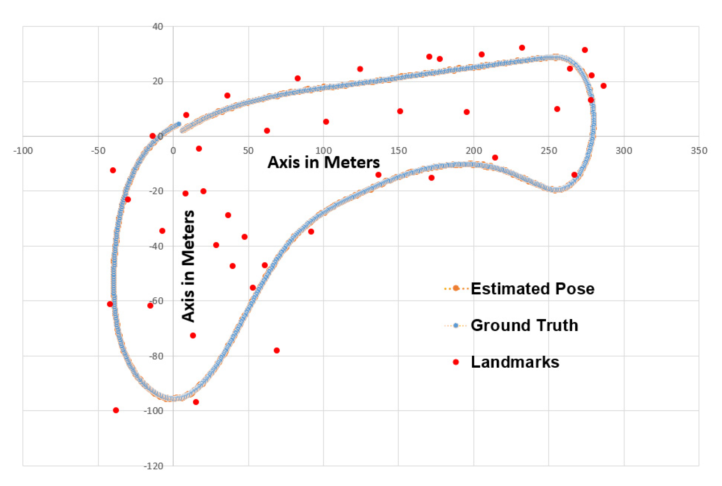
Moreover, through an iterative tuning process, the performance of the RTMCL is evaluated on several testing tracks while under various sets of hyperparameters. Figure 6 presents an example of one of the employed testing tracks. The length of this track is 754 m and has curvatures at several points. It also contains 42 landmarks that resemble poles to sufficiently emulate an urban driving environment.

The results of UKF testing performing the fusion of the lidar/radar are presented in

Table 4. The UKF’s performance assessment.

State Var	Cyclist	Car	Pedestrian	Pole
$p_x$	0.0648	0.1857	0.0652	0.0324
$p_y$	0.0809	0.1899	0.0605	0.0433
$v_x$	0.1452	0.4745	0.5332	0.0032
$v_y$	0.1592	0.5075	0.5442	0.0054
$\psi$	0.0392	0.2580	0.2075	0.0075

. Several objects are detected, including pole-like landmarks, cars, cyclists, and pedestrians. The five state variables, $p_x$, $p_y$, $v_x$, $v_y$, and $\psi$, are measured and their RMSE are listed in

Table 5. Assessment of the UKF performance for lidar/radar sensor fusion.

	Lidar + Radar	Lidar Only	Radar Only
RMSE-$p_x$	0.0648	0.1612	0.2031
RMSE-$p_y$	0.0809	0.1464	0.2539
RMSE-$v_x$	0.1452	0.2082	0.1971
RMSE-$v_y$	0.1592	0.2129	0.1871
RMSE-$\psi$	0.0392	0.0540	0.0480
NIS-Average	2.2797	1.6941	2.6576
NIS-Min	0.0012	0.04874	0.11309
NIS-Max	14.749	12.997	12.183
NIS > 95% Threshold	2.2%	3.2%	5.2%

as a KPI (Equation (26)). A comparison between the ground truth of each state variable to the estimated value of this state, then obtaining the error is performed by this KPI. Better detection is achieved with a lower value of this KPI.

The UKF is employed and tested in three different ways: the first one with only lidar signals, the second way with only radar signals, and the third one with the fusion between the lidar and the radar. This way of testing evaluates how significant the fusion is for the accuracy of object detection and tracking. Table 5 presents the results of the three ways of testing on the bicycle track. It is clear how significant the fusion is at all pose variables, all of them have much better RMSE. Table 5 clearly shows that fusion reduces the RMSE for all the pose state variables and makes a big difference in the accuracy of detection. As an example, the error of the detection position in the x-axis ($p_x$) is lowered by 60% compared to the one with the lidar alone and 70% compared to the one with radar alone. Another example is the error of the velocity detection in the x-axis ($v_x$) is lowered by 30% more than the one with the lidar alone and 26% more than the one with radar alone. Furthermore, the NIS KPI is computed as well for the three previous cases, showing that the fusion has significantly improved the UKF’s consistency. The fusion NIS quantities that are higher than the threshold of 95% have been lowered by 31% compared to the “only lidar” and 38.5% compared to the “only radar” values.

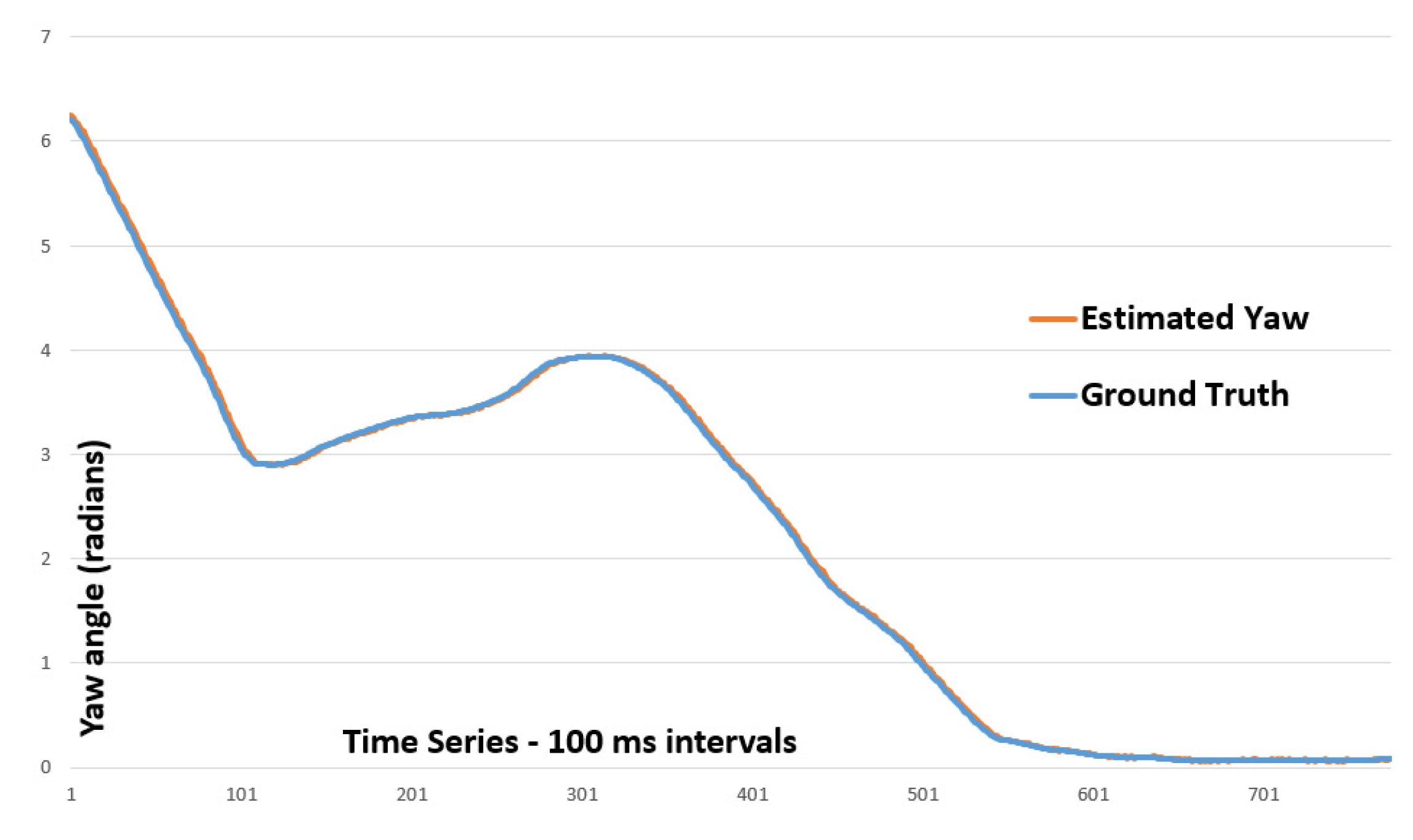
An example of testing the whole pipeline of the RTMCL, which includes the combination of the PF and UKF with the employment of the probabilistic reference map, Figure 6, Figure 7 and Figure 8 present the simulation results of egocar driving on the test track in Figure 6. The GB-DBSCAN is used for the data association step for the localization of the egocar on the global map. Figure 7 and Figure 8 show both the ground truth and the estimated egocar pose values drawn overlapping each other due to the computed small errors as reported in

Table 6. The PF uses numerous counts of particles.

# Particles	x-Error	y-Error	Yaw-Error	Exec. Time
15	122.34	33.002	1.5959	0.268 ms
25	0.1382	0.1240	0.0048	0.486 ms
50	0.1143	0.1154	0.0040	0.739 ms
100	0.1154	0.1071	0.0037	1.224 ms
150	0.1098	0.1060	0.0037	2.086 ms
200	0.1102	0.1039	0.0036	2.403 ms

Red is the worst-case scenario, green is the best-case, and # is no. of.

. The PF performance is evaluated using the RMSE KPI given in Equation (28). This KPI is computed for the three variables of the pose ($x$, $y$, and $\theta$). It evaluates each of these estimated values against its ground truth and aggregates the resulting errors. The performance of the PF is better if these KPI values are lower. Several counts of particles are used to choose the most appropriate configuration for the employed PF and to test its performance in real time. Hence, Table 6 shows that the minimum acceptable particle count is around 25 particles. Lower than this number, the PF starts to divert. However, to observe more robustness and improve further the accuracy, 50 particles are selected in this work to be employed by the PF, as higher numbers will not add much to the accuracy at the expense of much higher execution time. The count of 50 particles is considered a good balance between robustness and execution cost (real-time performance). The selection of 50 particles shows convergence in all the extensive performed tryouts.

The uncertainties in the reference map are modeled by the standard deviations associated with pole-like landmarks. The results of using the uncertainties in the map positions are reported in

Table 7. The influence of the landmark standard deviation.

${\mathit{\sigma }}_{{\mathit{x}}_{\mathit{p}\mathit{o}\mathit{l}\mathit{e}}}$	${\mathit{\sigma }}_{{\mathit{y}}_{\mathit{p}\mathit{o}\mathit{l}\mathit{e}}}$	x-Error	y-Error	Yaw-Error
0.3	0.3	0.1143	0.1154	0.0040
0.5	0.5	0.1730	0.1633	0.0057
1.0	1.0	0.2926	0.2736	0.0098

. Several standard deviations are tested and show how significantly it affects the final egocar pose estimation produced by the PF. The table shows that the RTMCL can handle a significant amount of uncertainty in the landmark position, which can reach up to 2.0 m or $2{\sigma }_{pole}$, and the computed error in the egocar localization is still below 30 cm.

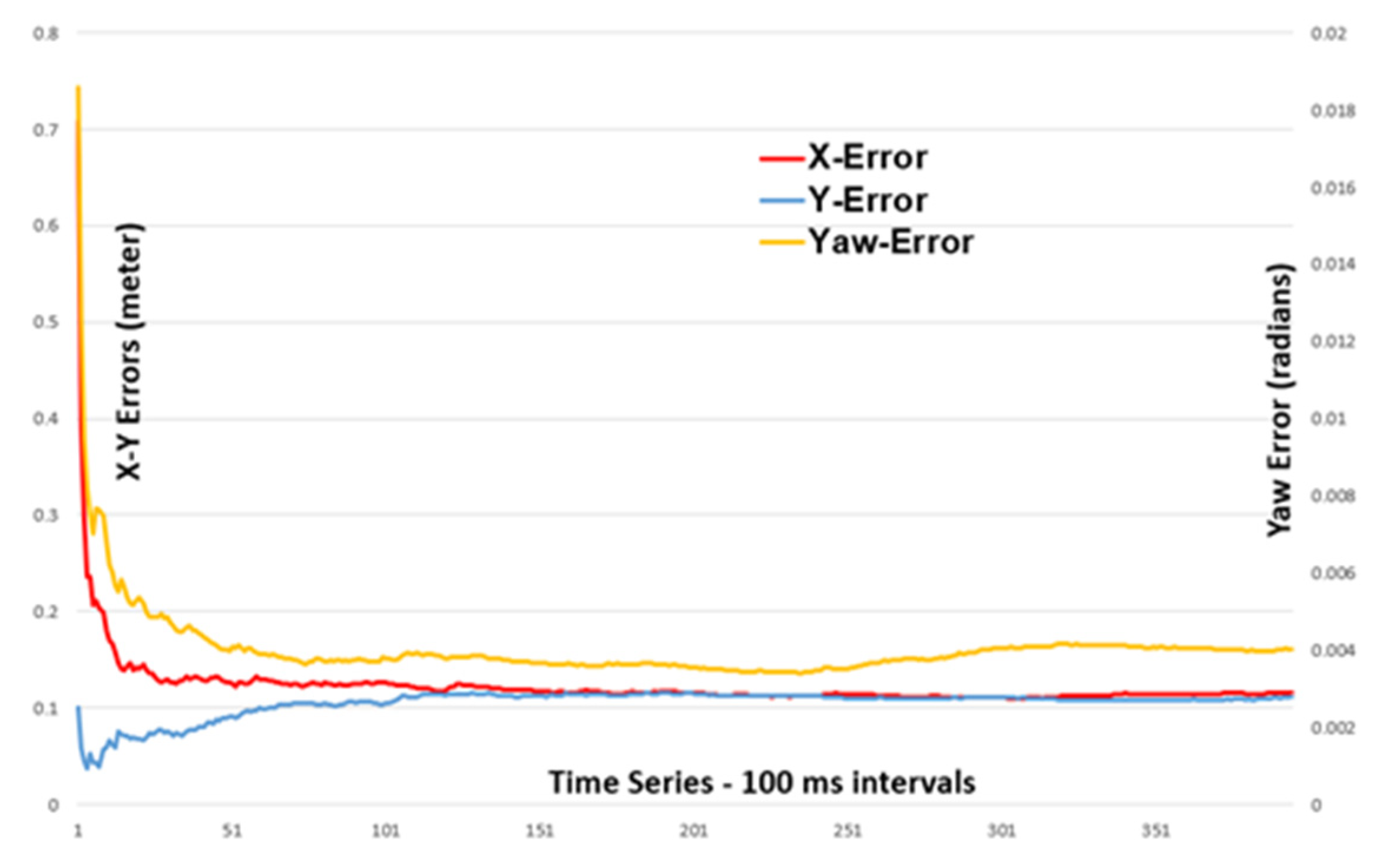
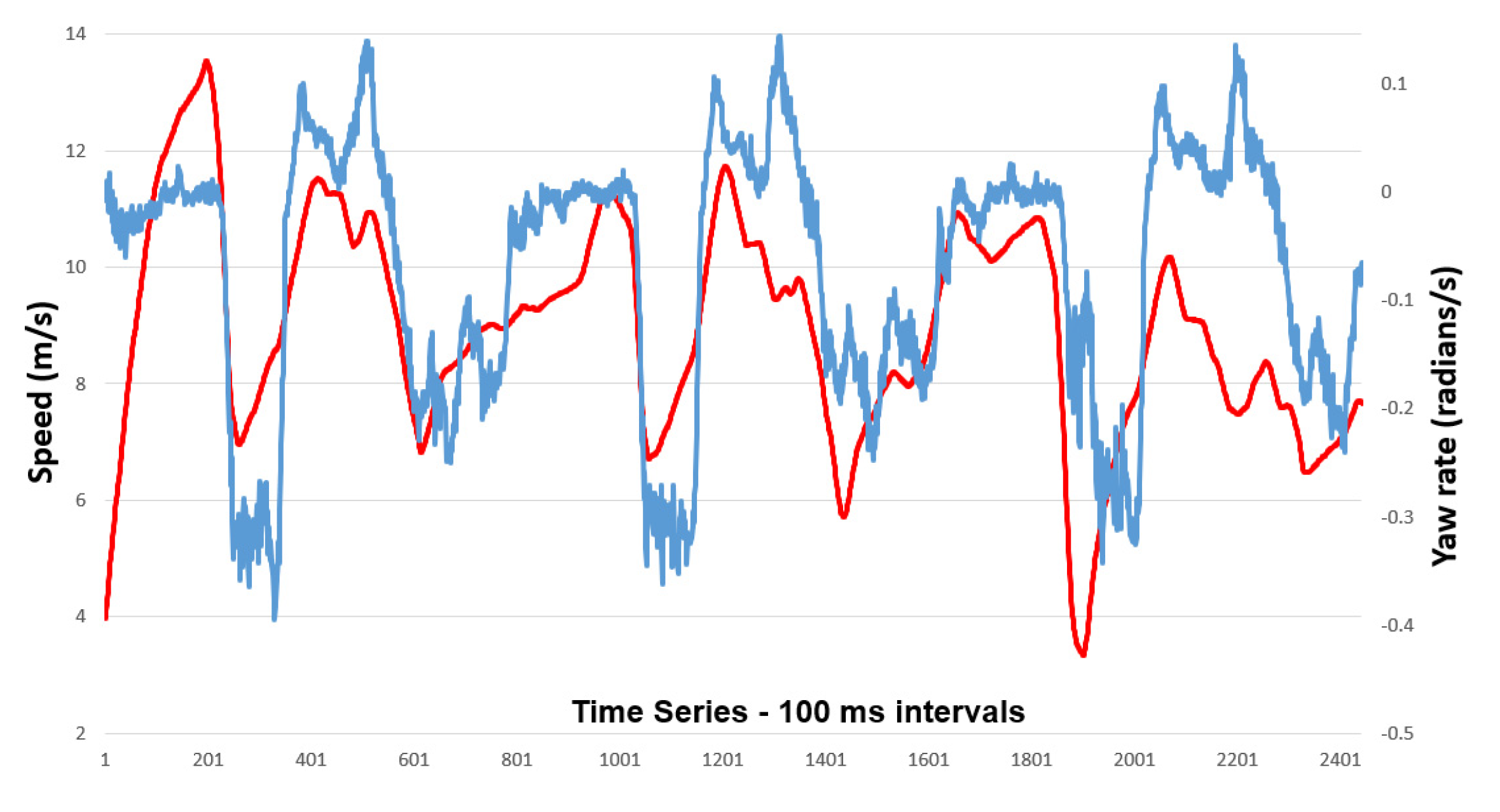
The performance of the PF during the start-up phase is very crucial for its convergence, stability, and performance later on. Therefore, Figure 9 presents the start-up segment of the PF employing 50 particles till it becomes stabilized (after around 100 time steps). As a sign or indicator of the robustness of the PF performance, Figure 10 presents the computed particles’ weights throughout a single lap driving on the test track. The best weight at each time step is significantly higher than the average weight. This is considered a good indicator of robustness [57].

It is observed that there is an inverse relation between these weight values (best and average) and the number of detected poles. Equation (30) below introduces another streamlined form of Equation (22), where the values of the weights are computed as the multiplication of the likelihoods of the observation of each pole-like landmark represented by a multivariate Gaussian probability density function. There is a suitable number of observed poles. If the number of observed poles is high, there is a chance that one or more of these poles have small Gaussian probability density values that can bring the whole product down and, consequently, the associated weight. After many tryouts, it is found that the most appropriate count of identified poles at each time step for the smooth operation of the RTMCL is in the scope of 4 to 12 poles as shown in Figure 11.

$$w_t^{\left[m\right]}={\prod }_{j=1}^N\frac{exp\left(-\frac{\left(z_{x_j}^{\left[t\right]}-{\mu }_{x_j}^{\left[t\right]}\right)}{2{\sigma }_{x_{pole}}^2}-\frac{\left(z_{y_j}^{\left[t\right]}-{\mu }_{y_j}^{\left[t\right]}\right)}{2{\sigma }_{y_{pole}}^2}\right)}{2\pi {\sigma }_{x_{pole}}{\sigma }_{y_{pole}}}$$

(30)

The real-time performance of the RTMCL is tested using extensive experimentation and tryouts proving that its execution is fast enough.

Table 8. Details of an individual pose estimation processing time by the RTMCL.

Process	Execution Time
State estimation by the UKF for 12 poles	12 × 439 μs
Clustering using GB-DBSCAN & RANSAC + data association using the ICP.	835 μs
Pose estimation by the Particle Filter	739 μs
Overhead by control tasks—20%	1368 μs
The sum of execution times	8210 μs

presents the measurements of the execution times of several tasks within the RTMCL pipeline on a very moderate computational platform: an Intel 1.6-GHz Core i5 with 8 GB of RAM. These measurements are collected for a single estimation of the egocar pose based on the 12-pole detection.

It is recommended from the literature that the localization pipeline iterates at a speed of 10 Hz to 30 Hz. Accordingly, the measured RTMCL execution time per iteration, which is 8.2 ms (122 Hz) in Table 8, is considered very well suited at even the upper limit of the recommendation.

Moreover, the values in Table 8 show that more than 50 pole detections can be employed and, still, the UKF is capable of meeting the requirements of collecting the lidar and radar measurements at a rate of 30 Hz (33.3 ms cycle) according to [1]. All the above analyses show that the real-time performance of the RTMCL is very convenient, allowing its robustness to be improved by either increasing the number of particles or allowing more pole detections.

Moreover, the results achieved in the work are significantly advantageous if compared with other works in the literature. The mean error for both the lateral and longitudinal positions (11 cm) is less than the 20 cm obtained in [58] using a pole-based reference map, stereo camera system as a main sensor, GPS as a secondary sensor, particle filter, and Kalman filter.

Additionally, the achieved mean error by RTMCL is also lower than the one achieved by [35], which is 16.4 cm (with an absolute max. error of 99.6 cm), obtained using a pole-based mapping, a lidar fused with RTK-GPS, IMU, wheel encoder, a Bayesian filter, and the egocar’s CTRV motion model.

Furthermore, the RTMCL outperforms the localization system proposed by [41], which fuses a digital map, GPS, and IMU, along with lanes and symbolic road markings (SRMs) recognized by a front camera via a particle filter. The latter-mentioned system produced a 95 cm longitudinal error and a 49 cm lateral error. The full comparative analysis is presented in

Table 9. Comparing the proposed approach with other stand-out methods.

Comparison Aspect	This Work (RTMCL)	(Spangenberg et al. [58])	(Weng et al. [35])	(Suhr et al. [41])
Mean Error (Lateral)	11 cm	20 cm	16.4 cm (Max: 99.6 cm)	49 cm
Mean Error (Longitudinal)	11 cm	20 cm	16.4 cm (Max: 99.6 cm)	95 cm
Sensor Configuration	GPS, IMU, radar, lidar, particle filter, Kalman filter.	Stereo camera, GPS, particle filter, Kalman filter	Lidar, RTK-GPS, IMU, wheel encoder, Bayesian filter.	Digital map, GPS, IMU, front camera.
Localization Approach	Real-Time Monte Carlo, Pole-based reference map, particle filter, Kalman filter.	Pole-based reference map, stereo camera, GPS, particle filter, Kalman filter.	Pole-based mapping, lidar, RTK-GPS, IMU, wheel encoder, Bayesian filter.	Digital map, GPS, IMU, front camera, particle filter.
Results Comparison	Significantly advantageous	20 cm mean error	16.4 cm mean error (Max: 99.6 cm)	95 cm longitudinal, 49 cm lateral error

below.

Moreover, the proposed RTMCL is compared to that of other research work based on fusion techniques, as summarized in

Table 10. Comparing the proposed approach with work based on other fusion techniques.

Aspect	Gao et al. [59]	Gao et al. [60]	Proposed Approach
Topic	Autonomous vehicle object detection.	Cyclist trajectory prediction.	Real-Time Monte Carlo Localization (RTMCL) for autonomous vehicles.
Methodology	Deep learning combining vision and lidar data.	Integrated framework with DBN and LSTM for cyclist intent prediction.	RTMCL with GPS, IMU, radar, and lidar data, incorporating clustering and particle filter techniques.
Key Techniques	Upsampling lidar, depth feature map, CNN.	DBN, LSTM with encoder-decoder, clustering algorithms	Particle filter, UKF, clustering algorithms, ICP.
Performance Metrics	Improved classification accuracy using fusion.	Predicts cyclist intentions within 0.9 s, and outperforms baseline methods.	Achieves 11 cm mean error, and handles uncertainties in pole-like landmark positions.
Implementation	Vehicle-mounted camera and lidar, NVIDIA® GeForce GTX Titan X, and NVIDIA® Jetson TX1	Lidar (Velodyne VLP-16, 10 fps) and a mono camera (IDS UI-5250CP-C-HQ, 15 fps).	Implemented in C++ on Intel 1.6-GHz Core i5 with 8 GB of RAM, real-time performance demonstrated.
Future Directions	Conduct real-world experiments based on a vehicle-mounted domain controller.	Explore cyclist-ego vehicle interaction, enhance robustness and interoperability	Add a front camera, incorporate additional road objects, and explore machine-learning approaches for improved localization.

. The first work discusses Gao et al.’s deep learning method for autonomous vehicle object detection [59], emphasizing the fusion of vision and lidar data to enhance classification accuracy. It highlights the upsampling of lidar point clouds, conversion into a depth feature map, and integration with RGB data for CNN input. The study employs a vehicle-mounted camera and lidar, using NVIDIA^® GeForce GTX Titan X and NVIDIA^® Jetson TX1 (NVIDIA, Santa Clara, CA, USA) for offline detection and classification on a public dataset.

The second work outlines Gao et al.’s integrated framework for predicting cyclist trajectories at unsignalized intersections [60]. It focuses on intent inference using a Dynamic Bayesian Network (DBN) considering motion, ego vehicle, and environmental features. The approach employs LSTM with encoder–decoder for online trajectory prediction, achieving predictions within 0.9 s of entering the intersection. The text underscores the approach’s outperformance over baseline methods (KF and DBN + KF) across various prediction horizons and its potential benefits for intelligent vehicles in road-user protection and path planning. Future research considerations include addressing cyclist–ego vehicle interaction and enhancing method robustness and interpretability.

11. Conclusions

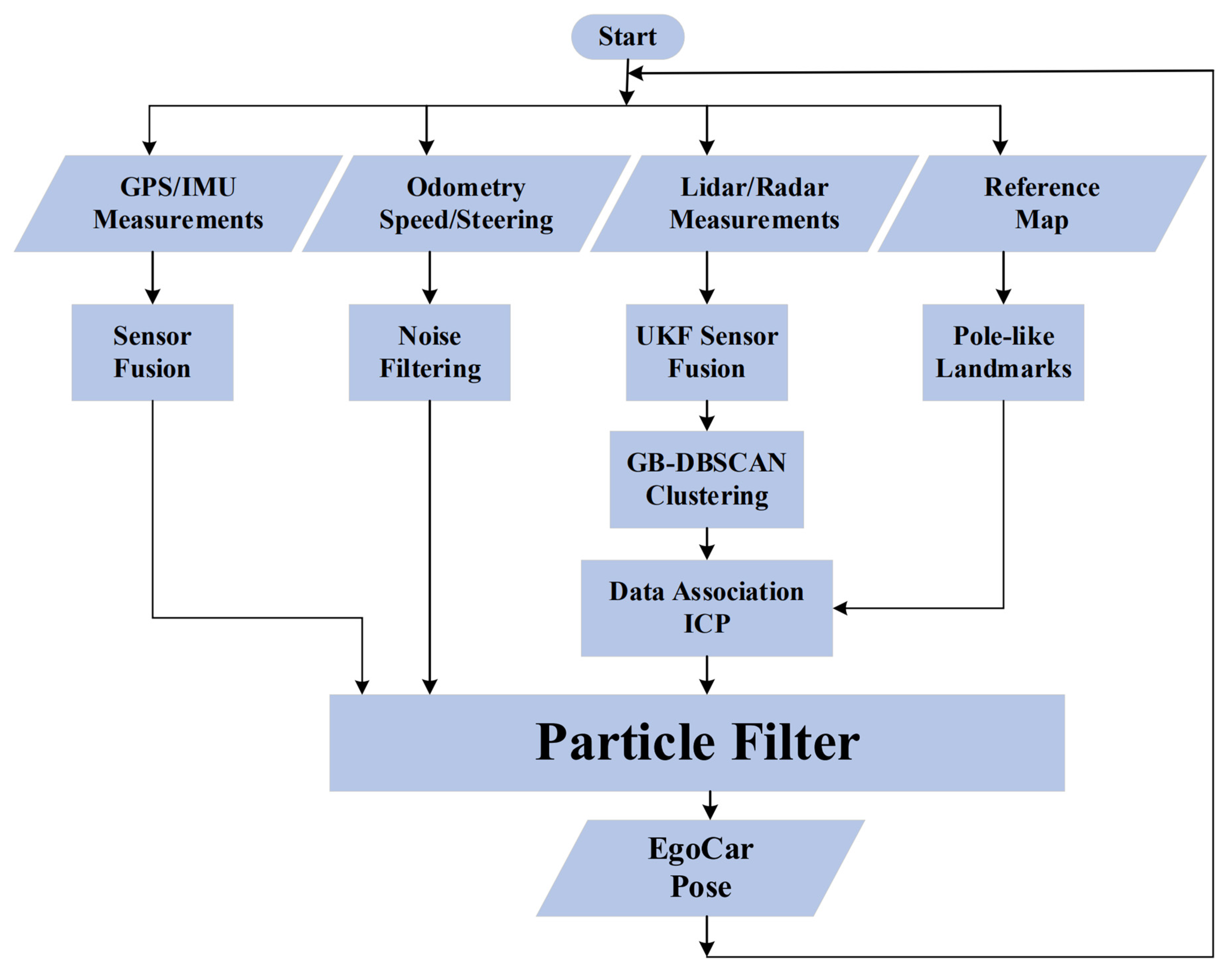
The proposed real-time Mont Carlo Localization (RTMCL) approach for self-driving vehicles is a pipeline of tasks that starts with the fusion between the GPS and the IMU to produce an unrefined egocar pose that is used to initialize the employed particle filter. Then, in the next task, a tailored UKF is used to fuse the collected data from the installed radar and lidar sensors on the egocar. The output of the UKF contains information about objects in the surrounding of the egocar and, thus, needs further processing to detect these objects and identify them. This task is carried out using the clustering algorithms GB-DBSCAN and RANSAC then produces the poses of the detected pole-like landmarks. In another task. The ICP algorithm is employed to perform the association between the identified poles in the previous task to the ones embedded in the provided reference map. In the final task, a tailored particle filter is developed and all the outputs of the previous tasks generate the fine-tuned egocar pose as the final localization measured reference to the co-ordinates of the global map.

The implementation of the whole RTMCL is conducted using C++ to ensure real-time performance. The testing results show that the RTMCL reached an accuracy of around 11 cm of mean error using merely 50 particles. The recorded execution times on affordable CPUs show the number of particles can further increase without much effect on the real-time performance.

Furthermore, testing the pipeline of the RTMCL has shown that it can run smoothly at 30 Hz while handling up to 50 poles at a time. Moreover, up to 2.0 m in uncertainty in the pose positions of the pole-like landmarks in the reference map can be handled successfully by the RTMCL, as its estimated egocar pose error will not exceed 30 cm in such a case.

It is planned to supplement a front camera as well as range finders [61] to the current fusion approach in the future and further examine the returns they will contribute to overall localization performance [62]. In addition, the RTMCL will be supplemented with additional road objects such as curbs, sidewalks, guardrails, and intersection features, among others. It is also worth considering the use of deep learning and other machine learning approaches.